TOMASZ KOZŁOWSKI1 MARTA KOLANKOWSKA2 ŁUKASZ WALASZCZYK3 Kielce University of Technology 1
e-mail:
[email protected] e-mail:
[email protected] 3 e-mail:
[email protected] 2
A FINITE DIFFERENCE SCHEME TO SOLVE ONE-DIMENSIONAL PROBLEMS ASSOCIATED WITH SOIL FREEZING AND THAWING Abstract
A finite difference scheme, which can be easily used for PC-programming to solve one-dimensional problems associated with soil freezing and thawing is presented. The method takes into account the real phase equilibria in the soil-water system, thereby being better interpretable both physically and in terms of soil mechanics. Some special computational procedures have been given, among them those relating to the crossing the freezing point and to determining the initial temperature distribution. Keywords: heat transfer, soil, phase changes, soil freezing point, unfrozen water content
Nomenclature a C cice cs cu erf G L Q t T Ta
– thermal diffusivity (m2 K-1) – volumetric heat capacity (J m-3 K-1) – specific heat of ice (J kg-1 K-1) – specific heat of dry soil (J kg-1 K-1) – specific heat of unfrozen water (J kg-1 K-1) – Gauss error function – geothermal gradient (K m-1) – latent heat of fusion of ice (J kg-1) – heat (J) – time (s) – temperature (K) – air temperature (oC)
T’
– fictional value of temperature ( C) o
1. Introduction Knowledge about the possible depth of frost or thaw in the subsoil is essential in a variety of problems in civil and environmental engineering. However, the existing analytical solutions are useful, as a rule, only in the cases of homogeneous and isotropic ground conditions [1]. Though some such methods deal with multilayer subsoil [1], they are still a little too flexible for most engineering computations. Instead, the numerical techniques are used for the calculation of the ground thermal regime. 34
Tf Tg w wu z wu z
– equilibrium freezing point (oC) – average annual temperature (oC) – water content (% of dry mass) – unfrozen water content (% of dry mass) – vertical coordinate (m) – unfrozen water content (% of dry mass) – vertical coordinate (m)
Greek symbols α rd
– convective heat transfer (W m-2 K-1) – soil dry density (kg m-3)
λ
– thermal conductivity (W/mK)
Dzi – vertical size of an element i (m)
A number of such methods have been developed during the last few decades. They cover solutions for oneand two-dimensional problems solved by the finite difference method (FDM) [2], [3] and in some cases by the finite element method (FEM) [4], [5], [6]. However, the characteristic features of the soil-water system, particularly relating to the phase phenomena (e.g. the freezing point depression and the unfrozen water content) are usually not taken into account, although the distribution of the latent heat of fusion plays a very
A FINITE DIFFERENCE SCHEME TO SOLVE ONE-DIMENSIONAL PROBLEMS ASSOCIATED WITH SOIL FREEZING ...
significant role in the thermal balance. When a simplified model, in which all water in the soil-water system freezes at 0oC is assumed, the obtained values of the depth of frost are under-predicted by up to 30% [7]. Moreover, in a number of the models some soil parameters are misapplied.In turn, the approximate analytic solutions do not take the temperature dependence of the soil phase composition into account. The aim of the paper is to present a finite difference scheme, which can be easily used for PCprogramming to solve one-dimensional problems associated with soil freezing and thawing. The method takes into account the real phase equilibriums in soilwater system, thereby being better interpretable both physically and in terms of soil mechanics. 2. Theory 2.1. The finite difference scheme The case of transient, geometric one-dimensional heat conduction will be discussed for a horizontally stratified region representing the ground (Fig. 1). Material properties within a given layer are uniform. Each layer is subdivided into a number of Dzi – sized elements, thereby establishing a grid with nodes 1, …, i, …, n in the centres of the elements. Thus the primary assumption made is that the temperature (or other properties) at nodal i represents the temperature over the entire element. In the region in question, the equation of transient, one-dimensional heat conduction with an internal heat source
δ 2T q g 1 δ T + = δ z2 l a δ t
(1)
is to be solved for time t > t0, whilst considering the boundary conditions at the top and the bottom. The initial temperature distribution Ti,0 for i = 1, 2, ...n is given. The general energy balance for an element i can be written, relating to the first law of thermodynamics, as
Qi +1, j + Qg ,i , j − Qi−1, j = Qs,i , j
(2)
where Qi+1,j is the heat entering the element from the lower side, calculated in relation to the state of the system in a time moment j (in the paper, the subscripts i and j denote the space and time coordinate respectively; in the case of time independent values, the time subscripts j will be omitted), Qg,i,j is the heat generated within the element, Qi-1,j is the heat leaving the element from the upper side and Qs,i,j is the heat stored in the element, the latter being an equivalent of the change of enthalpy.
Fig. 1. Discretization of one-dimensional heat transfer in stratified ground: a) division of the layers into final elements numbered 1,... i,... n, b) temperature Ti,j+1of the element i after a final time increment Dtj as a function of current temperatures of the element and of the adjacent elements
According to the widely known Fourier’s law of heat conduction and making use of the concept of thermal resistances, we can write
Qi+1, j =
Ti+1, j − Ti, j Dt Dzi +1 Dzi i , j + 2l i+1 2li
(3)
Ti, j − Ti −1, j Dt Dzi Dzi −1 i , j + 2li 2l i−1
(4)
and analogically
Qi−1, j =
To formulate the expression for the heat generated in an element i, the unfrozen water concept should be introduced. It is widely known that an amount of liquid water remains unfrozen in a soil water system in a wide range of temperatures beneath the freezing point Tf [8-11]. Thus,the temperature called the freezing point of soil water, in contrary to the freezing point of normal water in bulk, is comprehended as the temperature at which equilibrium freezing of liquid soil water (i.e. its solidification) begins. Any lowering of the temperature beneath the freezing point leads to the production of an amount of ice, which at any temperature T < Tf will remain in thermodynamic equilibrium with the unfrozen water. Oppositely, any increasing of the temperature melts an amount of ice, creating a new balance between liquid water and ice. A further increase in temperature will finally result in the melting of the last crystals of ice at the freezing 35
Tomasz Kozlowski, Marta Kolankowska, Łukasz Walaszczyk
point Tf. In other words, in the case of the soil-water system, the freezing point is the highest temperature at which ice is present in the system. Hence, the unfrozen water content wu, defined analogically to the water content w as the ratio of the mass of unfrozen water to the mass of dry soil, is a function of temperature:
w wu = wu (T )
T ≥ Tf T 0 Ci, j Dz i
(12)
which yields a restriction for time increment Dti,j:
Dt i , j >
C i, j Dzi Ai −1 Ai+1 2( Ai−1 + Ai+1 )
(13)
Below the freezing point, all the terms in Equation (9) have non-zero values. Additionally, the volumetric heat capacity Ci,j becomes temperature dependent. The temperature Ti,j+1 cannot be obtained in an explicit form and a special technique must be used to solve Equation (9). Another problem arises relating to the stability of Equation (9). The limitation of the time step set by the inequality (13) may now not guarantee the stability. Smith [13] shows that such a stability condition remains unaltered if the coefficient in the implicit FDM scheme depends linearly on the temperature. However, in the case of Equation (9), the temperature dependency follows from the unfrozen water content wu being a non-linear function of temperature. However, there is no need to establish the stability theoretically in
A FINITE DIFFERENCE SCHEME TO SOLVE ONE-DIMENSIONAL PROBLEMS ASSOCIATED WITH SOIL FREEZING ...
this case. According to Allen et al. [14], a possible approach consists in conducting a series of numerical experiments for a program based on the algorithm in question. The behaviour of the method over a spectrum of mesh geometries and coefficient values is examined and certain conclusions regarding the stability can be drawn. As will be shown below, the approach, often referred to as the heuristic stability analysis, has been applied in the case of the considered algorithm. The upper boundary condition will be established by assuming a fictional, additional node for which I = 0 and rewriting Equation (4):
Qi−1, j
T j − T0, j = 1, Dt D zi 1 1, j + 2l i a
(14)
where: a is the convective heat transfer coefficient, W/m2K, and T0,j refers to the air temperature. The lower boundary condition needs the introduction of the temperature of a fictional element n+1 outside the region in question:
Tn +1, j = Tn , j + G Dz n
(15)
where: G is the geothermal gradient, K/m. 2.2. Solution of the FDM scheme Basing on the FDM scheme presented in section 1, a PC-program Daisy 2.0 has been written enabling a complex thermal analysis of freezing and thawing ground. The applied step-by-step numerical procedure will be presented below. 1. Collecting data about the ground profile in question (thicknesses of layers, basic physical properties of soils). 2. Introducing the grid down to 8 m (it has been assumed that changes of temperature at this depth are negligible). 3. Establishing the initial temperature profile. It can be done by two alternate ways; the first one based on linear distribution from point to point, according to data provided by the user, and the second based on the Gauss error function, assuming that at the depth of 8 m the temperature is constant and equalled to the average annual temperature Tg for the region in question [15]:
z T ( z, t ) = Ta + (Tg − Ta ) erf l t 2 C
(16)
where: t is the length of a period, immediately before the simulation, for which the mean air temperature Ta is known. In Equation (16), the uniformity of the thermal properties over the entire profile is assumed. For the layered ground profile, the following recurrent procedure is proposed to establish the initial temperature distribution. The temperature in the first soil layer is calculated by use of the thermal parameters of this layer:
z T ( z,t ) = Ta + (Tg − Ta ) erf 2 l1,0 t C 1, 0
(17)
Temperature in a layer i is calculated as a function of the temperature Ti-1 at the lower boundary of the previous layer i-1, by use of the thermal properties of the layer i:
− k =i −1 hk z ∑ k =1 T ( z, t ) = Ti −1 + (Tg − Ti−1 ) erf 2 l i, 0 t Ci,0
(18)
The principle of the method is shown in Figure 2. For the purpose of numerical computations, the error function can be effectively approximated by the Taylor series:
erf x =
2 x3 1 x5 1 x7 x − + ⋅ − ⋅ + ... (19) 3 2! 5 3! 7 π
4. Collecting data about the thicknesses and physical properties of the insulating layers if any exist. 5. Collecting data about the air temperature as a number of pairs (T0,k,tk), where T0,k is a constant air temperature for the period of tk. 6. Computing the temperature independent thermal properties of soils in the profile: the freezing point Tf and the thermal conductivity l. 7. For the current temperature profile, computing the temperature dependent thermal properties of soils in every final element in the profile: the unfrozen water content and the volumetric heat capacity according to Equation (8). 8. For every final element i, computing the allowed time step with regard to the stability condition given by Equation (13) and then computing the minimal time increment for the stage j as 37
Tomasz Kozlowski, Marta Kolankowska, Łukasz Walaszczyk
Dt j = max{D ti , j ,i = 1...n}
(20)
Ti,j > Tf and Ti,j+1