Geosci. Model Dev., 9, 2909–2923, 2016 www.geosci-model-dev.net/9/2909/2016/ doi:10.5194/gmd-9-2909-2016 © Author(s) 2016. CC Attribution 3.0 License.
DebrisInterMixing-2.3: a finite volume solver for three-dimensional debris-flow simulations with two calibration parameters – Part 1: Model description Albrecht von Boetticher1,3 , Jens M. Turowski2 , Brian W. McArdell3 , Dieter Rickenmann3 , and James W. Kirchner1,3 1 Department
of Environmental Systems Science, ETH Zentrum, CHN H41, 8092 Zürich, Switzerland Potsdam GFZ German Research Center for Geosciences, Telegrafenberg, 14473 Potsdam, Germany 3 Swiss Federal Research Institute WSL, Zürcherstrasse 111, 8903 Birmensdorf, Switzerland 2 Helmholtz-Centre
Correspondence to: Albrecht von Boetticher (
[email protected]) Received: 26 June 2015 – Published in Geosci. Model Dev. Discuss.: 13 August 2015 Revised: 15 July 2016 – Accepted: 18 July 2016 – Published: 31 August 2016
Abstract. Here, we present a three-dimensional fluid dynamic solver that simulates debris flows as a mixture of two fluids (a Coulomb viscoplastic model of the gravel mixed with a Herschel–Bulkley representation of the fine material suspension) in combination with an additional unmixed phase representing the air and the free surface. We link all rheological parameters to the material composition, i.e., to water content, clay content, and mineral composition, content of sand and gravel, and the gravel’s friction angle; the user must specify only two free model parameters. The volume-of-fluid (VoF) approach is used to combine the mixed phase and the air phase into a single cellaveraged Navier–Stokes equation for incompressible flow, based on code adapted from standard solvers of the opensource CFD software OpenFOAM. This effectively singlephase mixture VoF method saves computational costs compared to the more sophisticated drag-force-based multiphase models. Thus, complex three-dimensional flow structures can be simulated while accounting for the pressure- and shear-rate-dependent rheology.
1
Introduction
Debris flows typically occur in steep mountain channels. They are characterized by unsteady flows of water together with different contents of clay, silt, sand, gravel, and larger particles, resulting in a dense and often rapidly moving mixture mass. They are often triggered by heavy rainfall and
can cause massive damage (Petley et al., 2007; Hilker et al., 2009). Their importance has increased due to extensive settlement in mountainous regions and also due to their sensitivity to climate change (Guthrie et al., 2010). Their damage potential is not limited to direct impact; severe damage can also be caused by debris flows blocking channels and thus inducing overtopping of the banks by subsequent flows (Tang et al., 2011). Modeling debris flows is a central part of debris-flow research, because measuring the detailed processes in debrisflow experiments or in the field is challenging. It is still uncertain how laboratory tests can be scaled to represent real flow events, and the inhomogeneous mixture of gravel and fine material brings about interactions of granular flow and viscous forces such as drag and pore pressure that are difficult to track with the present measurement techniques at reasonable cost. As a consequence, the rheological behavior of debris-flow material remains incompletely understood. Typically, current numerical modeling approaches cannot predict run-out distances or impact pressures of debris flows without parameter calibration that is based on simulations of previous well-documented events that occurred at the same site. This clearly represents a challenge in practical applications, because reliable calibration data are rarely available. Due to the complex physics of debris flows, real flows can only be accurately described by dynamical models that include strong phase interactions between granular and viscous fluid phases with several physical parameters (Pudasaini, 2012). From a practical application point of view and
Published by Copernicus Publications on behalf of the European Geosciences Union.
2910 guided by considerations of computational efficiency, here we neglect such phase interactions and restrict ourselves to an effectively single-phase mixture flow simulation. All currently applied debris-flow models that use a two-phase description of the debris-flow material are depth averaged or 2D. Three-dimensional debris-flow models with momentum exchange between phases have, up to now, been limited to academic cases due to their high numerical costs. Depthaveraged approximations are most applicable to flows over smooth basal surfaces with gradual changes in slope. These approximations are less valid when topography changes are abrupt, such as close to flow obstacles. They are also less applicable when the flow exhibits strong gradients in accelerations, such as during flow initiation and deposition, or in strongly converging and diverging flows. For such cases, we need a physically complete description of the flow dynamics without depth averaging (Domnik and Pudasaini, 2012). The essential physics of debris flows can be better retained by developing a full-dimensional flow model and then directly solving the model equations without reducing their dimension. The currently available models also contain many parameters that must be estimated based on measurements, or fitted to site-specific field data, limiting their applicability to real-world problems. Here, we provide a greatly simplified but effective solution linking the rheological model of the debris-flow material to field values such as grain size distribution and water content. The approach aims to link the knowledge of field experts for estimating the release volume and material composition with recent advances that account for complex flow phenomena, by using three-dimensional computational fluid dynamics with reasonable computational costs. The parameters of the two resulting rheology models for the two mixing fluids are linked to material properties such that the model setup can be based on material samples collected from the field, yielding a model that has two free parameters for calibration. One mixture component represents the suspension of finer particles with water (also simply called slurry in this paper) and a second component accounts for the pressuredependent flow behavior of gravel. The two components result in a debris bulk mixture with contributions of the two different rheology models, weighted by the corresponding component concentrations. A third gas component is kept unmixed to model the free surface. The focus is on the flow and deposition process and the release body needs to be user defined.
2
Modeling approach
The debris-flow material can be considered as a combination of a granular component and an interstitial fluid composed of a fine material suspension. The interstitial fluid was successfully modeled in the past as a shear-rate-dependent Herschel–Bulkley fluid (Coussot et al., 1998). Because presGeosci. Model Dev., 9, 2909–2923, 2016
A. von Boetticher et al.: DebrisFlowModel_I sure and shear drive the energy dissipation of particleto-particle contacts, the shear rate substantially influences the energy dissipation within the granular phase. While the two-phase models of Iverson and Denlinger (2001) and Pitman and Le (2005) treated the granular phase as a shearrate-independent Mohr–Coulomb plastic material, dry granular material has been successfully modeled as a viscoplastic fluid by Ancey (2007), Forterre and Pouliquen (2008), Balmforth and Frigaard (2007), and Jop et al. (2006). We follow the suggestions given by Pudasaini (2012) to account for the non-Newtonian behavior of the fluid and the shearand pressure-dependent Coulomb viscoplastic behavior of the granular phase, as proposed by Domnik et al. (2013). Several modeling approaches to account for the two-phase nature of debris flows used depth-averaged mass and momentum balance equations for each phase coupled by drag models (e.g., Bozhinskiy and Nazarov, 2000, Pitman and Le, 2005 and Bouchut et al., 2015). Pudasaini (2012) proposed a more comprehensive two-phase mass-flow model that includes general drag, buoyancy, virtual mass, and enhanced nonNewtonian viscous stress in which the solid volume fraction evolves dynamically. We apply a numerically more efficient method and treat the debris-flow material as one mixture (Iverson and Denlinger, 2001, Pudasaini et al., 2005a), with phase-averaged properties described by a single set of Navier–Stokes-type equations. The resulting reduction in numerical costs allows us to model the three-dimensional momentum transfer in the fluid as well as the free-surface flow over complex terrain and obstacles. We assume that the velocity of the gravel is the same as the velocity of the fluid. This assumption is motivated from application and would not be valid for general debris flows with interstitial fluid of low viscosity (i.e., a slurry with low concentration of fine material and large water content). The assumption of equal velocity of gravel and interstitial fluid in one cell leads to a constant composition of the mixture by means of phase concentrations over the entire flow process. This basic model can be seen as a counterpart to the mixture model of Iverson and Denlinger (2001), extended by resolving the three-dimensional flow structure in combination with a pressure- and shear-rate-dependent rheology linked to the material composition. The basic model presented here focuses on the role of pressure- and shear-rate-dependent flow behavior of the gravel, in combination with the shear-ratedependent rheology of the slurry. We base our model concept on the well-established finite volume solver interFoam, which is designed for incompressible two-phase flow simulations of immiscible fluids (Deshpande et al., 2012). A standard extension named interMixingFoam introduces two mixing phases without momentum exchange, coupled to a third unmixed phase by surface tension. The present method limits the physics of flow in terms of the interactions between phases such as drag, buoyancy, virtual mass, non-Newtonian viscous stress, and evolving volume fraction of the solid phase (Pitman and Le, 2005; www.geosci-model-dev.net/9/2909/2016/
A. von Boetticher et al.: DebrisFlowModel_I
2911
Table 1. Nomenclature. α αm ρ µ µ0 µmin µs σ κ Ddiff τy k n t p, pd γ˙ τ τ00 τ0 τ0s C P0 P1 β δ my φ U Uc g T, Ts D I ∇
phase fraction fraction of the debris mixture (slurry plus gravel) phase-averaged density, ρi (i = 1, 2, 3) density of phase i, ρexp is a bulk density in experiment phase-averaged dynamic viscosity, µi (i = 1, 2, 3) viscosity of phase i maximal dynamic viscosity minimal dynamic viscosity Coulomb viscoplastic dynamic viscosity free surface tension coefficient free surface curvature diffusion constant yield stress of slurry phase (τy−exp is a measured yield stress) Herschel–Bulkley consistency index Herschel–Bulkley exponent time pressure, modified pressure shear rate shear stress free model parameter (in slurry phase rheology) modified τ00 in case of high C yield stress of granular phase modeled with Coulomb friction volumetric solid concentration volumetric clay concentration reduced P0 in case of high clay content slope angle internal friction angle constant numerical parameter (in gravel phase rheology) volumetric flux (φρ denotes mass flux, φr a surface-normal flux) velocity interfacial compression velocity gravitational acceleration deviatoric viscous stress tensor, Cauchy stress tensor (s for granular phase) strain rate tensor identity matrix gradient operator
Pudasaini, 2012). Numerical costs are kept reasonable due to the volume-of-fluid (VoF) method (Hirt and Nichols, 1981), which solves only one Navier–Stokes equation system for all phases. The viscosity and density of each grid cell is calculated as a concentration-weighted average of the viscosities and densities of the phases that are present in the cell. Between the two mixing phases of gravel and slurry, the interaction reduces to this averaging of density and viscosity. In this way, the coupling between driving forces, topography and three-dimensional flow-dependent internal friction can be addressed for each phase separately, accounting for the fundamental differences in flow mechanisms of granular and viscoplastic fluid flow that arise from the presence or absence of Coulomb friction (Fig. 1). We apply linear concentrationweighted averaging of viscosities for estimating the bulk viscosity of a mixture for simplicity. Nevertheless, interacting forces such as drag between the grains and the fluid do not appear in our model because we set solid velocity equal to
www.geosci-model-dev.net/9/2909/2016/
fluid velocity, and thus, from the physical point of view, this is a debris bulk model. 2.1
Governing equations
Assuming isothermal incompressible phases without mass transfer, we separate the modeled space into a gas region denoting the air and a region of two mixed liquid components. The VoF method used here determines the volume fractions of all components in an arbitrary control volume by using an indicator function which yields a fraction field for each component. The fraction field represents the probability that a component is present at a certain point in space and time (Hill, 1998). The air fraction may be defined in relation to the fraction of the mixed fluid αm as α1 = 1 − αm ,
(1)
Geosci. Model Dev., 9, 2909–2923, 2016
2912
A. von Boetticher et al.: DebrisFlowModel_I
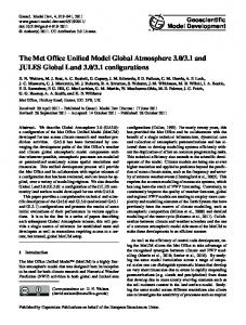
Figure 1. Viscosity distribution (indicated by color scale) along a 28 cm long section through the modeled 0.01 m3 release block 0.2 s after release, corresponding to the experimental setup of Hürlimann et al. (2015). The starting motion (black velocity arrows) with corresponding viscosity distribution of the mixture (left) is a consequence of blending pure shear-rate-dependent slurry-phase rheology (center) with the pressure- and shear-rate-dependent gravel phase rheology that accounts for Coulomb friction (right). Because the gravel concentration in this example is low, its effect on the overall viscosity is small.
and the mixed fluid αm may be defined as the sum of the constant fractions of the mixing phases α2 and α3 : αm = α2 + α3 .
(2)
The debris bulk motion is defined by the continuity equation together with the transport and momentum equations: ∇ · U = 0, ∂αm + ∇ · (U αm ) = 0, ∂t
(3) (4)
and ∂(ρU ) + ∇ · (ρU × U ) = −∇p + ∇ · T + ρf , ∂t
(5)
where t denotes time and U represents the debris bulk velocity field, T is the deviatoric viscous stress tensor for the mixture, ρ is the phase-averaged bulk density, p denotes pressure, and f stands for body forces per unit mass. We assume incompressible material and all fractions are convected with the same bulk velocity. Therefore, differences in phase velocities, and thus the interaction forces, such as drag between the grains and the fluid, are neglected. An efficient technique of the VoF method convects the fraction field αm as an invariant with the divergence-free flow field U that is known from previous time steps: ∂αm + ∇ · (U αm ) + ∇ · (α1 U c ) = 0, ∂t
(6)
where U c is an artificial interfacial compression velocity acting perpendicular to the interface between the gas region and the mixed liquid phases. The method allows a reconstruction of the free surface with high accuracy if the grid resolution is sufficient (Berberovi´c et al., 2009; Hoang et al., 2012; Deshpande et al., 2012; Hänsch et al., 2013). The details about the interface compression technique, the related discretization, and numerical schemes to solve Eq. (6) are given in Deshpande et al. (2012). However, to allow diffusion between the Geosci. Model Dev., 9, 2909–2923, 2016
mixing constituents of the slurry α2 and the gravel α3 in case of initially unequally distributed concentrations, our modified version of the interMixingFoam solver applies Eq. (6) separately to each mixing component including diffusion: ∂αi + ∇ · (U αi ) − Ddiff ∇ 2 αi + ∇ · (α1 U c ) = 0, ∂t
(7)
where i = 2, 3 denote the slurry and gravel constituents and Ddiff is the diffusion constant that is set to a negligible small value within the scope of this paper. The discrete form of Eq. (7) is derived by integrating over the volume V of a finite cell of a grid discretization of the simulated space, which is done in the finite volume method by applying the Gauss theorem over the cell faces. The advective phase fluxes φ1...3 are obtained by interpolating the cell values of α1 , α2 , and α3 to the cell surfaces and by multiplying them with the flux φ through the surface, which is known from the current velocity field. To keep the air phase unmixed, it is necessary to determine the flux φr through the interface between air and the debris flow mixture, and to subtract it from the calculated phase fluxes φ1...3 . Inherited from the original interMixingFoam solver (OpenFOAMFoundation, 2016a), limiters are applied during this step to bound the fluxes to keep phase concentrations between 0 and 1. With known fluxes φ1...3 , the scalar transport equation for each phase takes the form ∂ αi + ∇(φi ) − Ddiff ∇ 2 αi = 0. ∂t
(8)
Equation (8) is the implemented scalar transport equation solved for each constituent using first-order Euler schemes for the time derivative terms, as has been recommended for liquid column breakout simulations (Hänsch et al., 2013). After solving the scalar transport equations, the complete mass flux φρ is constructed from the updated volumetric fraction concentrations: φρ = φ1 ρ1 + φ2 ρ2 + φ3 ρ3 ,
(9)
www.geosci-model-dev.net/9/2909/2016/
A. von Boetticher et al.: DebrisFlowModel_I
2913
Figure 2. Longitudinal section through a debris-flow front discretized with finite-volume cells, showing the constitutive equations for one cell with density ρ and viscosity µ, given the densities ρ1...3 , viscosities µ1...3 , and proportions α1...3 of phases present. The numbers 1, 2, and 3 denote the air (white colored cell content), mud, and gravel phases, respectively.
where ρ1...3 denote the constant densities of the corresponding phases and φ1...3 are the corresponding fluxes. The complete mass flux φρ is used in the implementation to describe the second term of the momentum equation (Eq. 14) as described in Appendix A. Figure 2 illustrates how the phase volume distributions α1 (air), α2 (slurry), and α3 (gravel) are used to derive cell-averaged properties of the continuum. The conservation of mass and momentum is averaged with respect to the phase fraction α of each phase. The density field is defined as X ρ= ρi αi , (10) i
where ρi denotes density of phase i and the phase density is assumed to be constant. The deviatoric viscous stress tensor T is defined based on the mean strain rate tensor D that denotes the symmetric part of the velocity gradient tensor derived from the phaseaveraged flow field: 1 D = [∇U + (∇U )T ], 2
(11)
and T = 2µD.
(12)
Equation (12) was derived accounting for Eq. (3) and µ is the phase-averaged dynamic viscosity, which is simplified in analogy to Eq. (10) as the concentration-weighted average of the corresponding phase viscosities: µ=
X µi αi . i
www.geosci-model-dev.net/9/2909/2016/
(13)
With the continuity Eq. (3), the term ∇ ·T in Eq. (5) is written as ∇ · (µ∇U ) + (∇U ) · ∇µ to ease discretization. The body forces f in the momentum equation account for gravity and for the effects of surface tension. The surface tension at the interface between the debris-flow mixture and air is modeled as a force per unit volume by applying a surface tension coefficient σ . Although the surface tension can be considered to have a minor influence on debris-flow behavior, it allows an adequate reproduction of surface-flow patterns observed in laboratory-scale experiments used for validation (von Boetticher et al., 2015). The momentum conservation including gravitational acceleration g and surface tension is defined in our model as ∂(ρU ) + ∇ · (ρU × U ) = −∇pd + ∇ · (µ∇U ) ∂t + (∇U ) · ∇µ − g · x∇ρ + σ κ∇α1 ,
(14)
where κ denotes the local interfacial curvature and x stands for position. The modified pressure pd is employed in the solver to overcome some difficulties with boundary conditions in flow simulations with density gradients. In case the free surface lies within an inclined wall forming a no-slip boundary condition, the normal component of the pressure gradient must be different for the gas phase and the mixture due to the hydrostatic component ρg. It is common to introduce a modified pressure pd related to the pressure p by pd = p − ρg · x.
(15)
The gradient of the modified pressure includes the static pressure gradient and contributions that arise from the density Geosci. Model Dev., 9, 2909–2923, 2016
2914
A. von Boetticher et al.: DebrisFlowModel_I
gradient as well as a body force due to gravity (Berberovi´c et al., 2009). Together with the continuity Eq. (3), Eq. (14) allows us to calculate the pressure- and gravity-driven velocities. The corresponding discretization and solution procedure with the PISO (pressure-implicit with splitting of operators; Issa, 1986) algorithm is provided in Appendix A. The set of equations governing the flow in our model are Eqs. (8)–(15) together with the continuity Eq. (3). In the following section, we present the rheology models that define the viscosity components for Eq. (13).
state of the flow, the Herschel–Bulkley rheology law has been rarely applied in debris-flow modeling due to three rheology parameters. We avoid this problem by assuming some rheology parameters to be defined by measurable material properties as described below. Determination of rheology model parameters based on material properties
The viscosity of the gas phase, µ1 is chosen constant. The introduction of two mixing phases is necessary to distinguish between the pressure-dependent flow behavior of gravel and the shear-thinning viscosity of the suspension of finer particles with water. The rheology of mixtures of water with clay and sand can be described by the Herschel–Bulkley rheology law (Coussot et al., 1998), which defines the shear stress in the fluid as
Results from recent publications allow the reduction of the number of free Herschel–Bulkley parameters to two. If the coarser grain fraction is assumed to be in the gravel phase, the Herschel–Bulkley parameters for the finer material can be linked to material properties that can be measured using simple standard geotechnical tests. According to Coussot et al. (1998), the exponent n can be assumed constant at 1/3, and k can be roughly estimated as bτy , with the constant b = 0.3 s−n for mixtures with maximum grainsizes < 0.4 mm (Coussot et al., 1998). An approach for estimating the yield stress τy based on water content, clay fraction and composition, and the solid concentration of the entire debris-flow material was proposed by Yu et al. (2013) as
τ = τy + k γ˙ n ,
τy = τ0 C 2 e22(CP1 ) ,
2.2
Rheology model for the fine sediment suspension
(16)
where τy is a yield stress below which the fluid acts like a solid, k is a consistency index for the viscosity of the sheared material, γ˙ is the shear rate, and n defines the shearthinning (n < 1) or shear-thickening (n > 1) behavior. In OpenFOAM, the shear rate is derived in 3-D from the strain rate tensor D: √ γ˙ = 2D : D.
(17)
(18)
(19)
if the viscosity is higher, to ensure numerical stability. With n = 1, the model simplifies to the Bingham rheology model that has been widely used to describe debris-flow behavior in the past (Ancey, 2007). It may be reasonable to imagine the rheology parameters to be dependent on the state of the flow. However, even with the implicit assumption that the coefficients are a property of the material and not of the Geosci. Model Dev., 9, 2909–2923, 2016
+ 1.7Cmontmorillonite ,
(21)
where the subscript of C refers to the volumetric concentration (relative to the total volume of all solid particles and water) of the corresponding mineral. The discontinuity of P1 at a modified clay concentration of P0 = 0.27 is a coarse adjustment to a more-or-less sudden change observed in the experimental behavior. For C < 0.47, τ0 is equal to τ00 and otherwise τ0 can be calculated by τ0 = τ00 e5(C−0.47) ,
if the viscosity is below an upper limit µ0 and µ2 = µ0
where C (a constant) is the volumetric solid concentration of the mixture (the volume of all solid particles including fine material relative to the volume of the debris-flow material including water), P1 = 0.7P0 when P0 > 0.27, and P1 = P0 if P0