A Formal Model For Real-Time Parallel Computation Peter Hui
Satish Chikkagoudar
Pacific Northwest National Laboratory Washington, USA
[email protected] [email protected]
The imposition of real-time constraints on a parallel computing environment— specifically highperformance, cluster-computing systems— introduces a variety of challenges with respect to the formal verification of the system’s timing properties. In this paper, we briefly motivate the need for such a system, and we introduce an automaton-based method for performing such formal verification. We define the concept of a consistent parallel timing system: a hybrid system consisting of a set of timed automata (specifically, timed B¨uchi automata as well as a timed variant of standard finite automata), intended to model the timing properties of a well-behaved real-time parallel system. Finally, we give a brief case study to demonstrate the concepts in the paper: a parallel matrix multiplication kernel which operates within provable upper time bounds. We give the algorithm used, a corresponding consistent parallel timing system, and empirical results showing that the system operates under the specified timing constraints.
1
Introduction
Real-time computing has traditionally been considered largely in the context of single-processor and embedded systems, and indeed, the terms real-time computing, embedded systems, and control systems are often mentioned in closely related contexts. However, real-time computing in the context of multinode systems, specifically high-performance, cluster-computing systems, remains relatively unexplored. It can be argued that one reason for the relative dearth of work in this area is the lack of scenarios to date which would require such a system. Previously [11, 12], we have motivated the emerging need for such an infrastructure, giving a specific scenario related to the next generation North American electrical grid. In that work, we described the changes and challenges in the power grid driving the need for much higher levels of computational resources for power grid operations. To briefly summarize (and to provide some motivational context for the current work), many of these computations— particularly floating-point intensive simulations and optimization calculations ([2, 3, 8, 9, 10])—can be more effectively done in a centralized manner, and the amount and scale of such data is estimated by some [11, 12] to be on the order of terabytes per day of streaming sensor data (e.g. Phasor Measurement Units (PMUs)), with the need to analyze the data within a strict cyclical window (every 30ms), presumably with the aid of highperformance, parallel computing infrastructures. With this in mind, the current work is part of a larger research effort at Pacific Northwest National Laboratory aimed at developing the necessary infrastructure to support an HPC cluster environment capable of processing vast amounts of streaming sensor data under hard real-time constraints. While verifying the timing properties of a more traditional (e.g. embedded) real-time system poses complex questions in its own right, imposing real-time constraints on a parallel (cluster) computing environment introduces an entirely new set of challenges not seen in these more traditional environments. For example, in addition to standard real-time concepts such as worst-case execution time (WCET), realtime parallel computation introduces the necessity of considering worst case transmission time when ¨ C. Artho and P.C. Olveczky (Eds.): FTSCS 2012 EPTCS 105, 2012, pp. 39–55, doi:10.4204/EPTCS.105.4
Formal Model for RT Parallel Computation
40
communicating over the network between nodes, as well as the need to ensure that timing properties of one process do not invalidate those of the entire parallel process as a whole. These are but two examples of the many questions which must be addressed in a real-time parallel computing system; certainly there are many more questions than can be addressed in a single paper. To this end, we introduce a simple, event driven, automata-based model of computation intended to model the timing properties of a specific class of parallel programs. Namely, we consider SPMD (Single Program, Multiple Data), parent-child type programs, in part because in practice, many parallel programs— including many prototypical MPI-based [13, 15] programs— fall into this category. We give an example of such a program in Section 3. This model is typified by the existence of a cyclic master or parent process, and a set of noncyclic child or slave processes amongst which work is divided. With this characterization, a very natural correspondence emerges between the processes and the automata which model them: the cyclic parent process is very naturally modeled by an ω -automaton, and the child processes by a standard finite automaton. Our main contribution of this paper, then, is twofold: first, a formal method of modeling the respective processes in this manner, combining these into a single hybrid system of parallel automata, and secondly, a simple case study demonstrating a practical application of this system. We should note that the notion of parallel finite automata is not a new one; variants have been studied before (e.g. [6, 14]). We take the novel approach of combining timed variants ([1, 5]) of finite automata into a single hybrid model which captures the timing properties of the various component processes of a parallel system. The rest of the paper proceeds as follows: Section 2 defines the automaton models used by our system: Timed Finite Automata in Section 2.1, Timed B¨uchi Automata in Section 2.2, and a hybrid system combining these two models in Section 2.3. Section 3 gives a case study in the form of an example real-time matrix multiplication kernel, running on a small, four-node real-time parallel cluster. Section 4 concludes.
2
Formalisms
In this section, we give formal definitions for the machinery used in our hybrid system of automata. The definitions given in Sections 2.1 and 2.2 are not new [1]. However, it is still important that we state their definitions here, as they are used later on, in Section 2.3.
2.1 Timed Finite Automata In this section, we define a simple timed extension of traditional finite state automata and the words they accept. We will use these in later sections to model the timing properties of child processes in a real-time cluster system. Timed strings take the form (σ¯ , τ¯ ), where σ¯ is a string of symbols, and τ¯ is a monotonically increasing sequence of reals (timestamps). τx denotes the timestamp at which symbol σx occurs. We also use the notation (σx , τx ) to denote a particular symbol/timestamp pair. For instance, the timed string ((abc), (1, 10, 11)) is equivalent to the sequence (a, 1)(b, 10)(c, 11), and both represent the case where ‘a’ occurs at time 1, ‘b’ at time 10, and ‘c’ at time 11. Correspondingly, we extend traditional finite automata to include a set of timers, which impose temporal restrictions along state transitions. A timer can be initialized along a transition, setting its value to 0 when the transition is taken, and it can be used along a transition, indicating that the transition can only be taken if the value of the timer satisfies the specified constraint. Formally, we associate with each
P. Hui & S. Chikkagoudar
41
automaton a set of timer variables T¯ , and following the nomenclature of [1], an interpretation ν for this set of timers is an assignment of a real value to each of the timers in T¯ . We write ν [T 7→ 0] to denote the interpretation ν with the value of timer T reset to 0. Clock constraints consist of conjunctions of upper bounds: Definition 1. For a set T¯ of clock variables, the set X (T¯ ) of clock constraints χ is defined inductively as
χ := (T < c)? | χ1 ∧ χ2 where T is a clock in T¯ and c is a constant in R+ . While this definition may seem overly restrictive compared to some other treatments (e.g. [1]), we believe it to be acceptable in this early work for a couple of reasons. First, while simple, this sole syntactic form remains expressive enough to capture an interesting, non-trivial set of use cases (e.g. Section 3). Secondly, the timing analysis in subsequent sections of the paper becomes rather complex, even when timers are limited to this single form. Restricting the syntax in this manner simplifies this analysis to a more manageable level. We leave more complex formulations and the corresponding analysis for future work. Definition 2 (Timed Finite Automaton (TFA)). A Timed Finite Automaton (TFA) is a tuple hΣ, Q, s, q f , T¯ , δ , γ , η i , where • Σ is a finite alphabet,
• Q is a finite set of states, • s ∈ Q is the start state,
• q f ∈ Q is the accepting state,
• T¯ is a set of clocks,
• δ ⊆ Q × Q × Σ is the state transition relation,
• γ ⊆ δ × 2T is the clock initialization relation, and • η ⊆ δ × X (T¯ ) is the constraint relation. ¯
A tuple hqi , q j , σ i ∈ δ indicates that a symbol σ yields a transition from state qi to state q j , subject to the restrictions specified by the timer constraints in η . A tuple hqi , q j , σ , {T1 , ..., Tn }i ∈ γ indicates that on the transition on symbol σ from qi to q j , all of the specified timers are to be initialized to 0. Finally, a tuple hqi , q j , σ , X (T¯ )i ∈ η indicates that the transition on σ from qi to q j can only be taken if the constraint X (T¯ ) evaluates to true under the current timer interpretation. Example 3. The following TFA accepts the timed language {(ab∗ c, τ1 ...τn ) | τn − τ1 < 10} (i.e., the set of all strings consisting of an ‘a’, followed by an arbitrary number of ‘b’s, followed by a ‘c’, such that the elapsed time between the first and last symbols is no greater than 10 time units). The start state is denoted with a dashed circle, and the accepting state with a double line. b q1
a T=0
q2
c (T < 10)?
q3
Formal Model for RT Parallel Computation
42 Paths and runs are defined in the standard way:
Definition 4 (Path). Let A be a TFA with state set Q and transition relation δ . Then (q1 , ..., qn ) is a path over A if, for all 1 ≤ i < n, ∃σ .hqi , qi+1 , σ i ∈ δ .
Definition 5 (Run). A run r of a TFA hΣ, Q, q0 , q f , T¯ , δ , γ , η i over a timed word (σ¯ , τ¯ ), is a sequence of the form σ
σ
σ
σ
τ1
τ2
τ3
τn
3 1 2 n (q1 , ν1 ) −→ (q2 , ν2 ) −→ ... −→ (qn , νn ) r : (q0 , ν0 ) −→
satisfying the following requirements: • Initialization: ν0 (k) = 0, ∀k ∈ T¯ • Consecution: For all i ≥ 0: – δ ∋ hqi , qi+1 , σi i,
– (νi−1 + τi − τi−1 ) satisfies χi , where η ∋ hqi−1 , qi , σi , χi i, and – νi = (νi−1 + τi − τi−1 )[T 7→ 0], ∀T ∈ T¯ , where γ ∋ hqi , q j , σi , T¯ i r is an accepting run if qn = q f . A TFA A accepts a timed string s = (σ¯ , τ1 ...τn ) if there is an accepting run of s over A, and τn − τ1 is called the duration of the string. Note (Well-Formedness). We introduce a restriction on how timers can be used in a TFA, thus defining what it means for a TFA to be well-formed. Namely, we restrict timers to be used only once along a path; this is to simplify somewhat the timing analysis in subsequent sections. In particular, we say that a TFA A is well-formed if, for all pairs of states (qx , qy ), all timers T, and all paths from qx to qy , T is used no more than once. For example, the TFAs shown in Figure 1 are not well-formed, since in both cases, timers can potentially be used more than once— in the first case (A1 ), along the self-loop on q2 , and in the second case (A2 ), along two separate transitions along the path. At first, this may appear to be overly restrictive, but as it turns out, many of these cases can easily be rewritten equivalently to conform to the single-use restriction, as shown in Figure 2. b ; (T < 10)? a ; T=0 A1 :
q1
A2 :
q1
q2
a ; (T=0)? q2
c
q3
b ; (T < 10)? c ; (T < 20)? q3 q4
Figure 1: Malformed TFAs. Start states are denoted with a dashed circle, and accepting states with a double line. The intent of A1 is to allow strings of the form a, followed by arbitrarily many bs, as long as they all occur less than 10 units after the a, followed by a c. The intent of A2 is to allows strings of the form abc, where the elapsed time between the a and b is less than 10, and that between the a and c is less than 20. Both of these can be rewritten using conforming automata, as shown in Figure 2.
P. Hui & S. Chikkagoudar
43 b
A′1 :
a ; T=0 q1
b ; (T < 10)? q2a
q2b
c
q3
c A′2 :
q1
T1 = 0
q2
(T1 < 10)?
q3
(T2 < 20)?
q4
T2 = 0
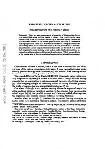
Figure 2: Equivalent, well-formed versions of automata from Figure 1. 2.1.1
Bounding Maximum Delay
An important notion throughout the remainder of the paper is that of computing bounds on the allowable delays along all possible paths through a TFA. Specifically, we are interested in doing so to be able to reason formally about the maximum execution time for a child process, with the end goal of being able to bound the execution time of the system— parent and all child processes— as a whole. The idea is that we will ultimately use TFAs to represent the timing properties of a child process. Paths through the automaton from its start state to an accepting state correspond to possible execution paths of the child process’ code. Certainly, proving a tight upper bound on the delay between two arbitrary points along an execution path remains a very difficult problem, but to be clear, this is not our goal. Rather, our approach involves modeling an execution path through a child process (and, by extension, its corresponding timed automaton) using an event-based model, in which selected system events are modeled by transitions in the automaton, and we rely on timing properties of the process to be guaranteed by the underlying RTOS process scheduler. The problem of computing the worst-case delay through the automaton equates to that of computing the maximum delay over all possible paths through the automaton from its start state to its accepting state: ∆A =
max p∈paths(A)
∆(p)
where • A = hΣ, Q, q0 , q f , T¯ , δ , γ , η i is the TFA • paths(A) denotes the set of all paths in A from its start state q0 to accepting state q f , and
• ∆(p), for path p = (q0 , ..., q f ), denotes the maximum delay from q0 to q f . That is, the maximum duration of any timed string (σ¯ , τ¯ ) such that (q0 ...q f , ν¯ ) is a run of the string over A (for some ν¯ ).
This problem can thus be formulated in the following manner: given a timed finite automaton A and an integer n, is there a timed word of duration d ≥ n that is accepted by A? While simple cases, such as those presented in this paper, can be computed by observation and enumeration, the complexity of the general problem remains an open question, although we highly suspect it to be intractable— Courcoubetis and Yannakakis give exponential-time algorithms for this and related problems, and have shown a strictly more difficult variant of the problem to be PSPACE-complete [4]. Furthermore, expanding the timer constraint syntax to a more expressive variant (c.f. [1]) can only complicate matters in terms of complexity. We must be cautious, then, to ensure that we do not impose an inordinately large number of timers on a child process.
Formal Model for RT Parallel Computation
44
¨ 2.2 Timed Buchi Automata Whereas we model the timing properties of the child processes of a cluster system using the timed finite automata of the previous section, we model these properties of the parent using a timed variant of ω -automata, specifically Timed B¨uchi Automata. We assume a basic familiarity with these; due to space constraints, we give only brief overview here. To review briefly, ω -automata, like standard finite automata, also consist of a finite number of states, but instead operate over words of infinite length. Classes of ω -automata are distinguished by their acceptance criteria. B¨uchi automata, which we consider in this paper, are defined to accept their input if and only if a run over the input string visits an accepting state infinitely often. Other classes of ω -automata exist as well. For example, Muller automata are more stringent, specifying their acceptance criteria as a set of acceptance sets; a Muller automaton accepts its input if and only if the set of states visited infinitely often is specified as an acceptance set. More detailed specifics can be found elsewhere— for example, [1]. A Timed B¨uchi Automaton (TBA) is a tuple hΣ, Q, q0 , q f , T¯ , δ , γ , η i, where • Σ is a finite alphabet,
• Q is a finite set of states, • q0 ∈ Q is the start state, • F ⊆ Q is a set of accepting states,
• T¯ is a set of clocks,
• δ ⊆ Q × Q × Σ is the state transition relation,
• γ ⊆ δ × 2T is the clock initialization relation, and ¯
• η ⊆ δ × X (T¯ ) is the constraint relation.
A tuple hqi , q j , σ i ∈ δ indicates that a symbol σ yields a transition from state qi to state q j , subject to the restrictions specified by the clock constraints in η . A tuple hqi , q j , σ , T¯ i ∈ γ indicates that on the transition on symbol σ from qi to q j , all clocks in T¯ are to be initialized to 0. Finally, a tuple hqi , q j , σ , X (T¯ )i ∈ η indicates that the transition on σ from qi to q j can only be taken if the constraint X (T¯ ) evaluates to true under the values of the current timer interpretation. We define paths, runs, and subruns over a TBA analagously to those over a TFA: Definition 6 (Path (TBA)). Let A be a TBA with state set Q and transition relation δ . (q1 , ..., qn ) is a path over A if, for all 1 ≤ i < n, ∃σ .hqi , qi+1 , σ i ∈ δ . Definition 7 (Run, Subrun (TBA)). A run (subrun) r, denoted by (q, ¯ ν¯ ), of a Timed B¨uchi Automaton hΣ, Q, q0 , q f , T¯ , δ , γ , η i over a timed word (σ¯ , τ¯ ), is an infinite (finite) sequence of the form σ
σ
σ
τ1
τ2
τ3
1 2 3 r : (q0 , ν0 ) −→ (q1 , ν1 ) −→ (q2 , ν2 ) −→ ...
satisfying the same requirements as given in Definition 5. For a run r, the set in f (r) denotes the set of states which are visited infinitely many times. A TBA T / where r is the run of w on A . A with final states F accepts a timed word w = (σ¯ , τ¯ ) if in f (r) F 6= 0, That is, a TBA accepts its input if any of the states from F repeat an infinite number of times in r. Example 8. Consider the following TBA A1 , with start state q1 and accept states F = {q1 }:
P. Hui & S. Chikkagoudar
45
c ; (T < 50)? b a;T =0 q1
q2
This TBA accepts the ω -language L1 = {((ab∗ c)ω , τ ) | ∀x.∃i, j.∀k.φ } where φ is the boolean formula
τi < τk < τ j =⇒ (σi = a) ∧ (σk = b) ∧ (σ j = c) ∧ (τ j − τi < 50) Lastly, we take the concept of maximum delay, introduced in the previous section with respect to Timed Finite Automata, and extend it to apply to Timed B¨uchi Automata. Doing so first requires the following definition, which allows us to restrict the timing analysis for TBAs to finite subwords: Definition 9 (Subword over q). ¯ Let A be a TBA, and let q¯ = (qm ...qn ) be a finite path over A . A finite timed word w = ((σm ...σn ), (τm ...τn )) is a subword over q¯ iff ∃q0 , ..., qm−1 , σ0 , ..., σm−1 , τ0 , ..., τm−1 such that (q0 ...qm−1 qm ...qn , ν¯ ) is a subrun of ((σ0 ...σm−1 σm ...σn ), (τ0 ...τm−1 τm ...τn )) over A for some ν¯ . Definition 9 is a technicality which is necessary to support the following definition of the maximum delay between states of a TBA: Definition 10. Let A be a TBA, and let q¯ be a finite path over A . Then ∆A (q) ¯ is the maximum duration of any subword over q. ¯ Example 11. Consider A1 from Example 8. Then ∆A1 (q1 q2 q2 q1 ) = 50. Algorithmically computing ∆A (q) ¯ for a TBA A is analogous to the case for TFAs; in small cases (i.e., relatively few timers with small time constraints), the analysis is relatively simple, while we conjecture the problem for more complex cases to be intractable; we leave more detailed analysis for future work.
2.3 Parallel Timing Systems Next, we model the timing properties of a SPMD-type parallel system as a whole by combining the two models of Sections 2.1 and 2.2 into a single parallel timing system. A parallel timing system (PTS) is a ¯ ψ , ϕ i, where tuple hP, A, • P = hΣ, Q, q0 , q f , T¯ , δ , γ , η i is a TBA (used to model the timing properties of the parent process) ¯ is a set {A1 , ..., An } of TFAs (used to model the timing properties of the child processes) • A ¯ is a fork relation (used to model the spawning of child processes) • ψ ⊆ δ ×A ¯ is a join relation (used to model barriers (joins)) • ϕ ⊆ δ ×A ¯ indicates that an instance of A is to be “forked” on the transition A tuple hqi , q j , σ , Ai in ψ , with A ∈ A, Ψ(A)
from qi to q j on symbol σ , and this “fork” is denoted graphically as qi −−−→ q j , modeling the spawning of a child process along the transition. Similarly, a tuple hqi , q j , σ , Ai in ϕ indicates that a previously forked instance of A is to be “joined” on the transition from qi to q j on symbol σ . This “join” is denoted Ω(A)
graphically as qi −−−→ q j , modeling the joining along the transition with a previously spawned child process1 . 1 Ψ was chosen as the symbol for ‘fork’, as it graphically resembles a “fork”; Ω was chosen as that for ‘join’, as it connotes “ending” or “finality”.
Formal Model for RT Parallel Computation
46
Example 12. Consider the following timing system S1 = hP, {A}, ψ , ϕ i: c ; (T < 50)? Ω(A)
b 0 ;U =0
a;T =0 q1
P:
q2
Ψ(A)
A:
s1
1 ; (U < 10)? s2
s3
P is the parent TBA with initial state q1 and final state set F = {q2 }. P accepts the ω -language L1 (see p. 45), and A is a TFA which accepts the timed language {(01, τ1 τ2 ) | τ2 − τ1 < 10}. In addition, the fork and join relations ψ and ϕ dictate that on the transition from q1 to q2 , an instance of A is forked (Ψ(A)), and that the transition from q2 to q1 can only proceed once that instance of A has completed (Ω(A)). Conceptually, this system models a parent process (P) which exhibits periodic behavior, accepting an infinite number of substrings of the form ab∗ c, in which the initial ‘a’ triggers a child process A which must be completed prior to the end of the sequence, marked by the following ‘c’. In addition, the ‘c’ must occur no more than 50 time units after the initial ‘a’. The child process is modeled by A, which accepts strings of the form 01, in which the 1 must occur no more than ten time units after the initial 0. In theory, child processes could spawn children of their own (e.g. recursion). For now, however, we disallow this possibility, as it somewhat complicates the analysis in the following section without adding significantly to the expressive power of the model. The model can be expanded later to allow for arbitrarily nested children of children with the appropriate modifications; specifically, TBAs would need to be extended to include their own ψ and ϕ relations, as would the definition of ∆ for TBAs. ¯ ψ , ϕ i is not itself interpreted as an Before proceeding, it is important to note that a PTS S = hP, A, automaton. In particular, we do not ever define a language accepted by S. Indeed, it is not entirely clear what such a language would be, as we never specify the input to any of the children in A. Rather, the sole intent in specifying such a system S is to specify the timing behavior of the overall system, rather than any particular language that would be accepted by it. 2.3.1
Consistency
With this said, we note that in Example 12, A is in some sense “consistent” with its usage in P. Specifically, since the maximum duration of any string accepted by A is 10, we are guaranteed that any instance a c of A forked on the q1 → − q2 transition will have completed in time for the ‘join’ along the q2 − → q1 transition and hence, the timer (T < 50)? on this transition would be respected in all cases. In this sense, all (Ψ(A), Ω(A)) pairs are consistent with timer T . However, such consistency is not always the case. Consider, for instance, the parallel timing system S2 shown in Figure 3. In this case, there are two child c ; (T < 25)? 0;U =0
Ω(B) a;T =0 P:
q1
Ψ(A)
A:
s1
B:
s1
0 ;V=0
b q2
Ω(A);Ψ(B)
1 ; (U < 10)? s2
q3
Figure 3: An inconsistent parallel timing system S2 .
s3
1 ; (V < 20)? s2
s3
P. Hui & S. Chikkagoudar
47
processes: A and B. The maximum duration of a timed word accepted by A is 10, and that of B is 20. Supposing that an ‘a’ occurs (and A forked) at time 0, it is thus possible that the A will not complete until time 10 − ε1 , at which time the ‘b’ and fork of B can proceed. It is therefore possible that B will not complete until time 30 − ε1 − ε2 (for small ε1 , ε2 ). This would then violate the (T < 25)? constraint, corresponding to a case in which a child process could take longer to complete than is allowable, given the timing constraints of the parent process. It is precisely this type of interference which we must disallow in order for a timing system to be considered consistent with itself. To this end, we propose a method of defining consistency within a timing system. Informally, we take the approach of deriving a new set of conditions from the timing constraints of the child processes, so that checking consistency reduces to the process of verifying that these conditions respect the timing constraints of the master process. ¯ ψ , and ϕ from the parallel timing system with a new set of derived timers, one First, we replace A, ¯ for each A ∈ A, defining the possible “worst case” behavior of the child processes. Each such timer TA is initialized on the transition along which the corresponding A is forked, and is used along (constrains) any transitions along which A is joined. Each such use ensures that the timer is less than ∆A , representing the fact that the elapsed time between the forking and joining of a child process is bounded in the worst case by ∆A — the longest possible duration for the child process. As an example, “flattening” the timing a system S1 of Example 12 results in a single new timer TA , initialized along the q1 − → q2 transition, and c used along the q2 − → q1 transition with the constraint (TA < 10)?. We then check that none of these new derived timers invalidate the timing constraints of the parent process. Formally, we define two relations. The first of these is flattening, which takes a parallel timing system ¯ ψ , ϕ i and yields a new pair of relations (γ , η ). Intuitively, γ defines the edges along which each hP, A, of the derived timers are initialized, and η defines the edges along which each of the derived timers are used: ¯ ψ , ϕ i be a parallel timing system. Then flatten(S) = (γ , η ), where Definition 13. Let S = hP, A,
γ = {hqi , q j , σ , {TA }i | hqi , q j , σ , Ai ∈ ψ } η = {hqi , q j , σ , X i | hqi , q j , σ , Ai ∈ ϕ } and X=
^
(TA < ∆A )
hqi ,q j ,σ ,Ai∈ϕ
The second relation takes ψ and ϕ as inputs and extracts a set of edge pairs, defined such that each such pair (e1 , e2 ) specifies when a derived timer is initialized (e1 ) and used (e2 ). ¯ Then the set of all use pairs ¯ ψ , ϕ i be a parallel timing system, with A ∈ A. Definition 14. Let S = hP, A, of A in S is defined as pairs(A, S) = {((qx , qy ), (qm , qn )) | (hqx , qy , σ1 , Ai ∈ ψ ) ∧ (hqm , qn , σ2 , Ai ∈ ϕ )} for some σ1 , σ2 . Furthermore, [ pairs(S) = pairs(A, S) ¯ A∈A
Example 15. Consider parallel timing system S3 shown in Figure 4. Observe that ∆A = 25 and ∆B = 11. Then: flatten(S3 ) = (γ , η ), where
γ = {hq1 , q2 , a, {TA }i, hq2 , q3 , b, {TB }i} η = {hq3 , q1 , c, X i} , where X = (TA < 25) ∧ (TB < 11)
Formal Model for RT Parallel Computation
48 q3
c P:
q1
T< ;(
)? 24
B) A, ( Ω a; T=0
Ψ(B)
b
t1 q2
Ψ(A)
0 ; V = 0 0 ; (V < 11)? t3 t2
B:
1 ; V = 0 ; (U < 20)?
1
0 ;U =0 s1
s5
s6 0
1 ; (V < 5)?
s2
s7
A:
0
s3
s4
< 0 ; (U
0
10)?
Figure 4: Parallel timing system S3 . ∆A = 25, ∆B = 11. shown graphically in Figure 5, and pairs(S) = pairs(A, S) ∪ pairs(B, S)
= {((q1 , q2 ), (q3 , q1 ))} ∪ {((q2 , q3 ), (q3 , q1 ))}
= {((q1 , q2 ), (q3 , q1 )), ((q2 , q3 ), (q3 , q1 ))} q3
c
q1
< ; (T
)? 24
(TB )∧ 5 2 < a A T ((