On the other hand, a number SR methods using CNN [14], .... CNN). Meanwhile, when the parallel algorithm is applied to. Proceedings of APSIPA Annual ...
Proceedings of APSIPA Annual Summit and Conference 2017
12 - 15 December 2017, Malaysia
A PARALLEL COMPUTATION ALGORITHM FOR SUPER-RESOLUTION METHODS USING CONVOLUTIONAL NEURAL NETWORKS Yusuke Sugawara∗ and Sayaka Shiota∗ and Hitoshi Kiya∗ ∗
Tokyo Metropolitan University Department of Information and Communication Systems 6-6 Asahigaoka, Hino-shi, Tokyo, JAPAN Abstract—An acceleration method for interpolation-based super-resolution (SR) methods using convolutional neural networks (CNNs), represented by SRCNN and VDSR, is proposed. In this paper, estimated pixels are classified into a number of types according to upscaling factors, and then SR images are generated by using CNNs optimized for each type. It allows us to adapt smaller filter sizes to CNNs than conventional ones, so that the computational complexity can be reduced for both running phase and training one. In addition, it is shown that the optimized CNNs for some type are closely related to those of other types, and the relation provides a method to reduce the computational complexity for training phase. A number of experiments are carried out to demonstrate that the effectiveness of the proposed method. The proposed method outperforms conventional ones in terms of the processing speed, while keeping the quality of SR images.
I.
INTRODUCTION
This paper addresses the problem of generating a highresolution (HR) image from given a low-resolution (LR) one, referred to as single image super-resolution (SR) [1]. Recently, learning-based SR methods, which model a mapping from LR to HR patches, have been widely studying for single image SR. The methods have various variations: neighbor embedding [2], sparse coding [3]–[6], random forest [7] and convolutional neural networks (CNNs) [8]–[15]. Among them, Dong et al. [8], [9] have demonstrated that a CNN can be used to learn a mapping from LR to HR in an end-to-end manner, and their method, referred to as SRCNN (super-resolution CNN), has the-state-of-the-art performance. Moreover, in order to achieve high accuracy, various SR methods using CNNs have been proposed such as very deep network [10], recurrence network [11] or training networks based on perceptual loss functions [12], [13]. Particularly, VDSR (Very Deep Network for SR) [10] and DRCN (DeeplyRecursive Convolutional Network) [11] can provide higher accuracy than that of SRCNN. However, most of these methods need huge calculation amount for training phase and testing one. On the other hand, a number SR methods using CNN [14], [15] have been proposed to reduce the calculation amount. Unfortunately, the SR methods provide lower quality than VDSR and DRCN, even though they reduce the calculation amount.
978-1-5386-1542-3@2017 APSIPA
Because of such a situation, an acceleration method for interpolation-based SR methods, represented by SRCNN, VDSR and DRCN, is proposed in this paper. Estimated pixels are classified into a number of types, and then SR images are generated by using CNNs optimized for each type. It enables to use smaller filter sizes than conventional ones, so that the calculation amount can be reduced for both running phase and training one. In addition, it is shown that the optimized CNNs for some type are closely related to those of other types. A number of experiments are carried out to demonstrate that the proposed method outperforms conventional ones in terms of the processing speed, while keeping the quality of SR images. II.
PREPARATION
This paper focuses on interpolation-based SR methods such as SRCNN [8], [9] and VDSR [10]. SRCNN and VDSR are summarized briefly, here. Our work aims to compute these methods in parallel to accelerate the processing. A. SRCNN SRCNN [9] directly learns an end-to-end mapping between LR/HR images as outlined in Fig. 1, where YL and Y are an LR image and a bicubic-interpolated LR one, and F (Y ), which is obtained by applying convolution operations of the third layer to the feature maps of the second one, is an output of the network i.e. an SR image. SRCNN consists of three layers: patch extraction/representation, non-linear mapping and reconstruction, and the filters have f1 × f1 = 9 × 9, f2 × f2 = 5 × 5 and f3 × f3 = 5 × 5, respectively as spatial sizes. For training, SRCNN directly models HR images. Given a training set {Y (i) , X (i) }N i=1 , the training of SRCNN is carried out to minimize the mean squared error 12 ∥F (Y ) − X∥2 averaged over the training set, where X is a ground truth HR image. Besides, It is trained for a single scale factor and is supported to work with the specified scale. B. VDSR VDSR [10] has been proposed as a higher accurate singleimage SR method. In order to achieve high accuracy, it uses a very deep convolution network whose model consists of 20 weight layers. In addition, an effective training procedure,
APSIPA ASC 2017
Proceedings of APSIPA Annual Summit and Conference 2017
HR image : 𝑌
𝑛1 feature maps : 𝐹1 (𝑌)
𝑛2 feature maps : 𝐹2 (𝑌)
𝑓2 × 𝑓2
𝑓1 × 𝑓1
SR image : 𝐹(𝑌)
12 - 15 December 2017, Malaysia
A1 A1
A2 A2
A1 A1
A2 A2
𝑓3 × 𝑓3
𝐴1 image 𝑋𝐴1 LR image : 𝑌𝐿
A3 A3
A4 A4
A3 A3
A4 A4
𝐴3 image 𝑋𝐴3 Layer2
Layer1 Bicubic Interpolation
Layer3
Division
A1 A 2 A1 A 2
A3 A4 A3 A4
Ground truth image 𝑋
𝐴4 image 𝑋𝐴4
Fig. 3: Image division for U = 2
Convolutional Neural Network Generating from ground truth Images
Fig. 1: SRCNN 𝑌𝐿
×4
LR image
𝑌𝑆
𝑌
×3 𝑌
×2 𝑌
𝐴2 image 𝑋𝐴2
A1 A 2 A1 A 2 A3 A4 A3 A4
A1 B1 B2 A2
A1 B1 A2
B3 C1 C2 B5
A1 A2
B2 C1 B3
B4 C3 C4 B6
A3 A4
A 3 B4 A 4
A 3 B7 B8 A 4
Type-𝐀𝟏 CNN Solver
Type-A1 image
𝑋𝐴1
Type-𝐀𝟐 CNN Solver
Type-A 2 image
𝑋𝐴2
Type-𝐀𝟑 CNN Solver
Type-A 3 image
𝑋𝐴3
Type-𝐀𝟒 CNN Solver
Type-A 4 image
𝑋𝐴4
Ground Truth image 𝑋 Division
Fig. 4: Parallel training for U = 2 (Basic principle) Fig. 2: upscaling for U = 2, 3 and 4
referred to as residual learning, has been proposed to improve the convergence speed, in which a multi-scale model is trained. The input to the network is a bicubic-interpolated LR image Y , and then convolution operations and ReLU [16] are applied to Y as well as SRCNN. In this paper, SRCNN and VDSR are reffed to as interpolation-based SR methods due to the use of the interpolated image Y as shown in Fig. 1.
LR image
𝑌𝐿
Type-𝐀𝟏 CNN
Type-A1 𝐹𝐴1 (𝑌𝐿 ) image
Type-𝐀𝟐 CNN
Type-A 2 𝐹𝐴2 (𝑌𝐿 ) image
Type-𝐀𝟑 CNN
Type-A 3 image
Type-𝐀𝟒 CNN
Type-A 4 𝐹𝐴4 (𝑌𝐿 ) image
SR image
𝐹(𝑌𝐿 ) Integration
𝐹𝐴3 (𝑌𝐿 )
Fig. 5: Parallel running for U = 2 (Basic principle)
C. Property of interpolation-based SR
An acceleration method for interpolation-based SR methods using CNNs is proposed, here. The proposed method enables to accelerate not only running phase but also training phase.
size than X, according to the relative positional relationship among pixels. Figure 3 illustrates the image division for U = 2, in which four small ground truth images, referred to as XAi , i = 1, 2, .., 4, are produced from X. Besides, an LR image YS is generated by downscaling the ground truth image X. Next, four CNNs corresponding to four types are independently trained by using YS and XAi , i = 1, 2, .., 4 as shown in Fig.4. 2) Running Phase The procedure to generate SR images is illustrated in Fig. 5. An LR image YL is entered into four trained CNNs as their inputs, and four SR images FAi (YL ), i = 1, .., 4 are outputted from four CNNs, respectively. Finally, an SR image F (YL ) with full size is generated by integrating them, in which the integration operation corresponds to the reverse one of the image division in Fig. 3.
A. Outline of proposed parallel computation algorithm
B. PSRnet and PVDSRnet
1) Training Phase In the proposed method, firstly, each ground truth HR image X is divided into a number of ground truth images with smaller
When the above parallel algorithm is applied to SRCNN, we name it PSRnet (Parallel Computation for Super-Resolution CNN). Meanwhile, when the parallel algorithm is applied to
Several highly accurate SR methods such as SRCNN and VDSR input interpolated images to a network. As shown in Fig. 2, the SR methods can be interpreted as methods of estimating surrounding pixels for each pixel in an LR image YL [17]. In this paper, the estimated pixels are classified into a number of types, according to the relative positional relationship like Ai , i = 1, 2, .., 4 for upscaling factor U = 2 as shown in Fig. 2, and then SR images are generated by using CNNs optimized for each type. In addition, it will be shown that the optimized CNNs for some type are closely related to those of other types in this paper. III.
PROPOSED METHOD
978-1-5386-1542-3@2017 APSIPA
APSIPA ASC 2017
Proceedings of APSIPA Annual Summit and Conference 2017
12 - 15 December 2017, Malaysia
VDSR, it is referred to as PVDSRnet (Parallel Computation for Very Deep CNN). Let us consider PSRnet in more detail. The space resolution of input images for PSRnet is lower than that for SRCNN, so that PSRnet can use smaller filters due to a difference in receptive field sizes. The receptive field size of SRCNN, RF S is given by 3 ∑ RF S = f1 + (fl − 1). (1) l=2
𝑅𝑜𝑡−90
𝑅𝑜𝑡270 (𝑌𝐿 )
Type-𝐀𝟏 CNN
𝑅𝑜𝑡−270 Type-A 𝐹𝐴3 (𝑌𝐿 ) 3
Type-𝐀𝟏 CNN
𝑅𝑜𝑡−180 Type-A 𝐹𝐴4 (𝑌𝐿 ) 4
𝑅𝑜𝑡180 (𝑌𝐿 )
Input image
image
image
(p)
Ground truth image 𝑋
A1 A 2
A1 A1
A1 A1
↓𝐀 𝟏
𝐴1 image 𝑋𝐴1
𝑌𝑆
A3 A4 Original image 𝑋
CNN(0° )
Rot90
Rot90
↓𝐀 𝟏
CNN Solver
𝑅𝑜𝑡90 (𝑋)
↓ 𝐴1 (𝑅𝑜𝑡90 𝑋 )
CNN(90° )
(mod(⌈ fUl ⌉, 2)=1) ⌈ fUl ⌉, ⌈ fUl ⌉ + 1 or ⌈ fUl ⌉ − 1, (mod(⌈ fUl ⌉, 2)=0). (p)
Ground truth image
Type-A1 CNN Solver
LR image
should satisfy, in each layer, (4)
(p)
Considering (3) and (4) together, (f1 , f2 , f3 ) = (5, 3, 3) is given for U = 2 from both equations. A similar approach is also avalable for desinging the size of each filter in VDSR. C. Parallel training with rotated data It is shown that the optimized CNN for some type is closely related to those of other types. As a result, the computational complexity of training phase can be reduced by using the relation. 1) Using rotated LR images A parallel training approach and a parallel running one were described in Figs. 4 and 5 respectively. Let us consider the parallel running again to eliminate some redundancy. Figure 6 illustrates another approach for parallel running. In this figure, rotated LR images and only one CNN are used, even though four CNNs are needed in Fig. 5, where the operator Rotθ (YL ) denotes to rotate image YL by θ degrees, as illustrated in Fig. 7. This parallel approach allows us to train only one CNN for generating SR images for U = 2, so that the computational cost for the training can be reduced. Note that three CNNs are required to be trained for U = 3 and U = 4, because estimated pixels are classified roughly into three types according to the relative positional relationship like Ai , Bi and Ci as shown in Fig. 2. Figure 7 illustrates a parallel training approach with rotated images. Type-A1 CNN namely, CNN(0◦ ) leans a mapping between YS and XA1 , and CNN(90◦ ) is trained to learn a
978-1-5386-1542-3@2017 APSIPA
𝐹(𝑌𝐿 )
Type-A2 𝐹𝐴2 (𝑌𝐿 ) image
Integration
𝑅𝑜𝑡90 (𝑌𝑆 )
l=2
(p) fl =
Type-𝐀𝟏 CNN
LR image
For U = 2, RF S (p) = 9 is obtained from (2). The size of (p) each filter in PSRnet fl should meet the equation, as well as in (1), 3 ∑ (p) (p) RF S (p) = f1 + (fl − 1) (3) In addition, {
LR 𝑌𝐿 image
𝑅𝑜𝑡90 (𝑌𝐿 )
SR image
Fig. 6: Proposed parallel running with rotated LR images
When (f1 , f2 , f3 ) = (9, 5, 5) is chosen, (1) provides RF S = 17 [10]. Meanwhile, the receptive field size of PSRnet, RF S (p) is expressed as, { S S (mod(⌈ RF ⌈ RF U ⌉, U ⌉, 2) = 1) RF S (p) = (2) S S ⌈ RF (mod(⌈ RF U ⌉ + 1, U ⌉, 2) = 0).
(p) fl
Type-A1 𝐹𝐴1 (𝑌𝐿 ) image
Type-𝐀𝟏 CNN
Fig. 7: Parallel training with rotated ground truth images ■ indicates position A1
mapping between Rot90 (YS ) and ↓ A1 (Rot90 (X)), where the operator ↓ A1 (X) denotes to decimate image X at position A1 . Thus, XA2 in Fig. 3 satisfies the relation ↓ A1 (Rot90 (X)) = Rot90 (XA2 ).
(5)
This relation suggests that the two CNNs learn the same mapping. In other words, CNN(0◦ ) is closely related to other CNNs as CNN(90◦ ), CNN(180◦ ) and CNN(270◦ ), so that this relation allows us to reduce the computational complexity of the training phase. The proposed parallel running in Fig. 6 is given by this insight. 2) Augmentation with Rotated Data CNN(0◦ ) and CNN(90◦ ) in Fig. 7 learn the same mapping, so that the training dataset {Rot90 (YS ),Rot90 (XA2 )} can be used for training CNN(0◦ ). Thus, other training sets such as {Rot270 (YS ),Rot270 (XA3 )}, {Rot180 (YS ),Rot180 (XA4 )} and so on can be used for training CNN(0◦ ) as well. This method is easily extended to for U = 3 and U = 4. In addition, this augmentation method can be combined with the conventional data augmentation [18]. IV.
EXPERIMENTAL RESULTS
We apply the proposed parallel algorithm to SRCNN and VDSR to demonstrate the effectiveness. That is, PSRnet and PVDSRnet are compared with SRCNN and VDSR, respectively.
APSIPA ASC 2017
Proceedings of APSIPA Annual Summit and Conference 2017
12 - 15 December 2017, Malaysia
TABLE I: Comparison with state-of-the-arts (PSNR (dB), SSIM, RunningTime (sec)) test dataset Set5
Set14
upscaling factor ×2 ×3 ×4 ×2 ×3 ×4
Bicubic PSNR/SSIM/time 33.66/0.9299/ 30.39/0.8682/ 28.42/0.8104/ 30.23/0.8687/ 27.54/0.7736/ 26.00/0.7019/ -
SRCNN [9] PSNR/SSIM/time 36.90/0.9554/1.98 32.75/0.9105/1.98 30.44/0.8636/1.98 32.49/0.9073/3.88 29.20/0.8208/3.88 27.36/0.7494/3.88
A. Datasets for Training and Testing We employ 91-image set from Yang et al. [3] as our training dataset, which is widely used in other learning-based SR methods. In addition, the same data augmentation (rotation and downscaling) as in [15] is used. As a result, a training set consisting of 1820 images, referred to as 91-image-Aug, is created for our experiments. Besides, we use two datasets as test datasets. Set5 [2] and Set14 [6], which are often used for benchmark in other works, are employed. B. Training Parameters and Benchmark For benchmark, we follow the public available framework of Huang et al. [19]. It enables the comparison of many state-ofthe-art results with the same evaluation procedure. The framework applies bicubic interpolation to color components of an image and sophisticated models to luminance components as in other methods [9]–[11]. To prepare a training set, we first downscale HR images by desired factors as 2, 3, or 4 and create LR images as YS . 1) PSRnet (p) (p) (p) For PSRnet, filters have the sizes (f1 , f2 , f3 ) = (5, 3, 3) for U = 2, which are decided by (2), (3) and (4), while the filters of SRCNN have the sizes (f1 , f2 , f3 ) = (9, 5, 5) [9], where other parameters are the same as those of SRCNN. Note that the complexity of (9, 5, 5) is over twice of (5, 3, 3). The LR images YS are cropped into 33 × 33 pixel patches and the ground truth images XA1 are also cropped as well as YS , where a stride is also selected as in other methods [8] [9]. As a result, the total number of patches per one CNN is over 35, 000. In addition, we apply zero padding in all layers according to filter sizes as in the methods [10], [11], [15]. For training phase, Adam [20] is employed as an optimizer where the learning rates are 10−3 for the first and second layers and 10−4 for the third one. Adam can achieve faster convergence than the stochastic gradient descent(SGD) used in SRCNN and others. We train with a batch size of 128 for 1000k iterations. The filter weights of the convolutional layers are initialized with the method described in [21]. All models are implemented by using the Caffe framework [22]. 2) PVDSRnet For PVDSRnet, filters have the sizes for U = 2, { 3 ( l = 1, 3, · · · , 19 ) (p) fl = (6) 1 ( l = 2, 4, · · · , 20 )
PSRnet PSNR/SSIM/time 37.07/0.9564/0.738 32.98/0.9122/0.650 30.58/0.8657/0.540 32.64/0.9085/1.48 29.38/0.8225/1.32 27.54/0.7518/1.08
VDSR [10] PSNR/SSIM/time 37.21/0.9576/22.0 33.06/0.9169/22.0 30.67/0.8739/22.0 32.49/0.9068/65.2 29.28/0.8237/65.2 27.49/0.7555/65.2
PVDSRnet PSNR/SSIM/time 37.30/0.9577/6.59 33.08/0.9156/4.71 30.78/0.8714/3.81 32.80/0.9102/12.4 29.37/0.8246/9.64 27.67/0.7574/7.69
TABLE II: Comparison of Training Time (hour) for U = 2 Training Time
SRCNN
PSRnet
VDSR
PVDSRnet
26.57
10.18
40.00
25.31
For training, the patch size is 41 × 41. Besides, the batch size is 64, and SGD is used under momentum= 0.9 and weight decay= 0.0001. The learning rate is initially set to 0.1 and then decreased by a factor of 10 every 20 epochs by 80 epochs. The weight initialization method [21] is employed, and the threshold value θ for the adjustable gradient clipping proposed in [10] is set to 0.1. PVDSRnet is trained for each upscaling factor. C. Comparison with state-of-the-arts In order to have fair comparison, the training conditions of PSRnet and PVDSRnet are assigned to SRCNN and VDSR as the conditions, respectively. All results for running phase are summrized in Table I. The running time is tested using the Caffe implementation on a PC, with a 4.00 GHz CPU and a main memory of 8GB. The result shows that PSRnet and PDVSRnet outperform SRCNN and VDSR in terms of the processing speed, respectively. The quality of SR images for proposed method is almost the same or higher than conventional ones. Table II shows the training time for U = 2 on GPU Quadro K5200. This table presents that the proposed method enables to accelerate not only the running time but also the training time. V.
CONCLUSION
This paper addressed an acceleration method for interpolationbased SR methods using CNNs. The proposed method allows us to utilize CNNs with filters of smaller sizes than SRCNN and VDSR, and to carry out the running phase with rotated data in parallel. As a result, the computational complexity can be reduced for both running phase and training one. The proposed parallel processing can be applied to SRCNN and VDSR, and PSRnet and PVDSRnet was proposed as new SR methods. The experimental results demonstrated that the proposed method outperforms conventional ones in terms of processing speed, while keeping the quality of conventional SR images.
while the filters of VDSR have fl = 3 for all layers.
978-1-5386-1542-3@2017 APSIPA
APSIPA ASC 2017
Proceedings of APSIPA Annual Summit and Conference 2017
R EFERENCES [1] C.-Y. Yang, C. Ma and M.-H. Yang, “Single-image super-resolution: A benchmark,” in Proc. European Conference on Computer Vision (ECCV), 2014, pp. 372–386. [2] M. Bevilacqua, A. Roumy, C. Guillemot and M. L. Alberi-Morel, “Lowcomplexity single-image super-resolution based on nonnegative neighbor embedding,” in Proc. British Machine Vision Conference (BMVC), 2012. [3] J. Yang, J. Wright, T. S. Huang and Y. Ma, “Image super-resolution via sparse representation,” IEEE Transactions on Image Processing, vol. 19, no. 11, pp. 2861–2873, 2010. [4] R. Timofte, V. De and L. V. Gool, “Anchored neighborhood regression for fast example-based super-resolution,” in Proc. IEEE International Conference on Computer Vision (ICCV), 2013, pp. 1920–1927. [5] R. Timofte, V. De Smet and L. Van Gool, “A+: Adjusted anchored neighborhood regression for fast super-resolution,” in Proc. IEEE Asian Conference on Computer Vision (ACCV), 2014, pp. 1920–1927. [6] Zeyde, Roman and Elad, Michael and Protter, Matan, “On single image scale-up using sparse-representations,” in Proc. Curves and Surfaces, 2010, pp. 711–730. [7] S. Schulter, C. Leistner and H. Bischof, “Fast and accurate image upscaling with super-resolution forests,” in Proc. IEEE Conference on Computer Vision and Pattern Recognition (CVPR), 2015, pp. 3791– 3799. [8] C. Dong, C. C. Loy, K. He and X. Tang, “Learning a Deep Convolutional Network for Image Super-Resolution,” in Proc. European Conference on Computer Vision (ECCV), Springer, 2014, pp. 184–199. [9] C. Dong, C. C. Loy, K. He and X. Tang, “Image super-resolution using deep convolutional networks,” IEEE Transactions on Pattern Analysis and Machine Intelligence, vol. 38, no. 2, pp. 295–307, 2016. [10] J. Kim, J. K. Lee and K. M. Lee, “Accurate image super-resolution using very deep convolutional networks,” in Proc. IEEE Conference on Computer Vision and Pattern Recognition (CVPR), 2016, pp. 1646– 1654. [11] J. Kim, J. K. Lee and K. M. Lee, “Deeply-recursive convolutional network for image super-resolution,” in Proc. IEEE Conference on Computer Vision and Pattern Recognition (CVPR), 2016, pp. 1637– 1645. [12] A. A. J. Johnson and F. Li, “Perceptual losses for real-time style transfer and super-resolution,” in Proc. European Conference on Computer Vision (ECCV), 2016, pp. 694–711. [13] C. Ledig, L. Theis, F. Huszar, J. Caballero, A. P. Aitken, A. Tejani, J. Totz, Z. Wang and W. Shi, “Photo-realistic single image super-resolution using a generative adversarial network,” in Proc. IEEE Conference on Computer Vision and Pattern Recognition (CVPR), 2017. [14] W. Shi, J. Caballero, F. Huszar, J. Totz, A. P. Aitken, R. Bishop, D. Rueckert and Z. Wang, “Real-time single image and video superresolution using an efficient sub-pixel convolutional neural network,” in Proc. IEEE Conference on Computer Vision and Pattern Recognition (CVPR), 2016, pp. 1874–1883. [15] C. Dong, C. C. Loy and X. Tang, “Accelerating the super-resolution convolutional neural network,” in Proc. European Conference on Computer Vision (ECCV), Springer, 2016, pp. 391–407. [16] A. L. Maas, A. Y. Hannun, and A. Y. Ng, “Rectifier nonlinearities improve neural network acoustic models,” in Proc. ICML Workshop on Deep Learning for Audio, Speech, and Language Processing, 2013. [17] S. Ohtani, Y. Kato, N. Kuroki, T. Hirose and M. Numa, “Superresolution with four parallel convolutional neural networks,” IEICE TRANSACTIONS on Information and Systems, vol. J99-D, no. 5, pp. 588–593, 2016 (in Japanese). [18] A. Krizhevsky, I. Sutskever and G. E. Hinton, “Imagenet classification with deep convolutional neural networks,” in Proc. Advances in Neural Information Processing Systems (NIPS), 2012, pp. 1097–1105. [19] J.-B. Huang, A. Singh and N. Ahuja, “Single image super-resolution from transformed self-exemplars,” in Proc. IEEE Conference on Computer Vision and Pattern Recognition (CVPR), 2015, pp. 5197–5206. [20] D. P. Kingma and J. Ba, “Adam: A method for stochastic optimization,” in Proc. International Conference on Learning Representations (ICLR), 2015. [21] K. He, X. Zhang, S. Ren and J. Sun, “Delving deep into rectifiers: Surpassing human-level performance on imagenet classification,” in Proc. IEEE International Conference on Computer Vision (ICCV), 2015, pp. 1026–1034.
978-1-5386-1542-3@2017 APSIPA
12 - 15 December 2017, Malaysia
[22] Y. Jia, E. Shelhamer, J. Donahue, S. Karayev, J. Long, R. Girshick, S. Guadarrama and T. Darrell, “Caffe: Convolutional architecture for fast feature embedding,” arXiv preprint arXiv:1408.5093, 2014.
APSIPA ASC 2017