The use of small intervals preserves the interaction between the distortion ... We also describe a FORTRAN computer program called FAW that implements the.
NRL Memorandum Report 4413
A FORTRAN Computer Program for Calculating The Propagation of Plane, Cylin.rical, or Spherical Finite Amplitude Waves D.H.
TPIVElT AND
A.L.
VAN BUREN
UnderwaterSound Reference Detachment Naval Research Laboratory P.O. Box 833 7, Orlando, FL 32856
L
:. ..
.
February i9, 1981
' -. )
LJU
NAVAL RESEARCH LABORATORY Washington, D.C. Approved for public release; distribution unlimited.
2
23
3
-ECu,.CLASSIFICA rION OF THJ-
PAGE (When
le Entered)
REPORT DOCUMENTAIONREAD REPORT DOCUMENTATION PAGEt: I
NUMBER
INSTRUCTIONS BEFORE COMPLETING FORM
. GOVT ACCESSION NO.
NRI Memorandume
413
3.
RECIPIENT'S CATALOG NUMBER
S
TYPE OF REPORT & PERIOD COVERED
W
TITLf (and Sub te)
S
(a
TUInterim i~D.BI OMPUTFR ORAM FOR ;ALCULATING THE OPAGATIOK OFYLANE 9YLINDRICA' ,OR CG-PHERICAL INITEMPLrDF ANE WAVESL i'EtfU
rio
OO(s)
6
PERFORMING ORG. REPORT NUMBER
B.
CONTRACT OR GRANT NUMBER(s)
D. H Trivett Mif'A. L. Van Buren PERFORMING ORGANIZ ATION NDetachment AME AND ADDRESS Underwater Sound Reference
+9
-" i~ "P.O0. z
report on a continuing NLpolm
10.
RME
MENT.NPROJECT. TASK
~ ~~Naval Research
LaboratoryN Box 8337, Orlando, FL 32856
1t
CO N T R O L L IN G O F F IC E N A MEC A J .
61153N R D
E S
'l
_
Q
ONR via NRL Code 5000 Washigton D.C.
R 'l -' 1i gt2 0591-0
ZE
r, -'
12
F
:
2n03c751.
EUIY
LS.
otisrp
37 14
MONITORING AGENCY NAME
r15. Chi
SECURITY CLASS. (of
rport)
UNCLASSIFIED ISa.
OECLASSIFICATION/DOWNGRADING SCHEDULE
16.
DISTRIB
M
Approved for public release; distribution unlimited.
17. DISTRIBUTION STATEMENT (of the abstract entered In Block 20, If different from Report)
IS
SUPPLEMENTARY NOTES
19
KEY WORDS (Continue on reverse side it necessary md identify by block number)
Nonlinear acoustics
Computer program
Finite amplitude wave Nonlinear wave
Propagation Burgers'equation
20. AB TRACT (Continue on reverse old& If necesary and Identify by block number)
A numerical solution to the generalized Burgers' radial wave equation has been developed; it allows oeii to calculate stepwise the harmonic content of a finite amplitude wave in the frequency domain for the case of plane. cylindrical, or spherical geometry. The finite amplitude wave may have any initial harmonic content with arbitrary phase, and the absorption coefficient of each harmonic is independently adjustable. Remaining in the frequency domain allows a much larger step than conventional algorithms, which alternate between the time and frequency domains. A listing of the computer program is included.
DD
73
1473
5-
EDITION OF I NOV 65 IS OBSOLETE SS
9.iS0 ± -
=7=
SI
PG R
CIi2AIOTHPG.66Oa
(UNe Dat5 Enter
II CONTENTS
INTRODUCTION . .
.
.
.
.
.
.
.
.
.
.
.
.
.
.
.
.
.
.
.
2
.................
I.
THEORY
II.
RELATIVE IMPORTANCE OF LINEAR ABSORPTION AND NONLINEAR EFFECTS ...................
.
.
.
.
.
.
.
.
....
A.
Series Truncation . . . .
B.
Integration
C.
Variable Step Size
D.
Renormalization . . . .
IV.
DESCRIPTION OF COMPUTER PROGRAM FAW .
.
.
.
.
.
......
A.
Significant FORTkAN Variable Names
.
.
.
.
.
.
.
B.
Major Computation Blocks in FAW .
C.
Parameter Input . . . . .
.
.
.
.
.
.
.
D.
Printed Output
. . . . .
.
.
.
.
.
.
.
E.
Number of Harmonics ..............
F.
Step Size . . ...............
V.
COMPARISON WITH PHENOMENOLOGICAL MODEL ..
Method
. ......... . .
5
.................
III. NUMERICAL IMPLEMENTATION
.
.
.
.....
.7
.
.
. . .....
.
.
.
.
.....
.........
APPENDIX A - Computer Program FA1 APPENDIX B - Sample Output from FA1
. . .
9
.
10 11 12
. .
.
.
.
. .....
18
.
.
.
......
20 20
......
.
.
..........
.
21 22
.
........
...............
.
.
.
.
.
16
.
.
.
8
.....
.......
REFERENCES . ....................
EiN
.
.
24 25 34
I A FORTRAN COMPUTER PROGRAM FOR CALCULATING THE PROPAGATION OF PLANE, CYLINDRICAL, OR SPHERICAL FINITE AMPLITUDE WAVES INTRODUCTION
II
Several adequate theories [1,2,3], based on approximations to the nonlinear wave equation, have been developed to describe the behavior of a one-dimensional wave of moderate amplitude as it propagates through a nonlinear fluid.
Most of these theories, however, are not conveniently applied to the
problem of describing the propagation when the wave is of arbitrary initial waveform or when the linear absorption has an arbitrary frequency dependence. To handle these more general case:, investigators [4,5,61 have adapted the phenomenological model of Fox and Wallace [71 to use a high-speed computer to calculate the propagation stepwise.
The distance of propagation in this
model is divided into small intervals.
The wave is first allowed to distort
over one interval and is then corrected to account for absorption and geometrical
spreading. interval.
The procedure is then repeated for the new waveform over the next The use of small intervals preserves the interaction between the
distortion, the absorption, and the geometrical spreading mechanisms.
Since
the distortion mechanism is applied in the particle velocity domain with absorption and geometrical spreading being applied in the frequency domain, it is necessary to switch back and forth between the two domains during each step.
Even with the use of the Fast Fourier Transform (FFT), this procedure
is a time-consuming process.
In addition, one must take special care in
applying the distortion mechanism when the waveform has a very steep shock-like portion.
We describe in this report a new procedure for calculatLng the propagation of plane, cylindrical, or spherical finite amplitude waves. This procedure performs the stepwise calculations entirely in the frequency domain, thus avoiding both the use of the FFT and the steep waveform problems. We also describe a FORTRAN computer program called FAW that implements the new procedure.
The theory behind the procedure is described in Sec. I.
A discussion
of the relative importance of linear absorption and nonlinear effects is presented in Sec. II.
In Sec. III the numerical implementation of the procedure
Manuscript bubmitted November 24, 1980.
J
!1
is
This is followed in Sec. IV b3 a description of the computer
developed.
program FAW.
Included are discussions of the significant FORTRAN variable
names, the major computational blocks, parameter input, printed output, number of harmonics required in the calculation, and initial step size. Section V contains a comparison of results obtained using the new procedure with results obtained using the phenomenological model.
The report concludes
with appendices containing sample output and a program listing of FAW.
I.
THEORY An approximate nonlinear wave equation valid for one-dimensional and
progressive plane, cylindrical, and spherical waves in a lossless fluid is the generalized Burgers' equation [8] U U + (a/r)U - bU _ = 0,
()
where U = particle velocity, r = spatial coordinate, T = retarded time (t co
r
-- r
small signal sound speed,
b =
2
/c2 0
= (i +
B
), the nonlinearity parameter, and
a = 0 (plane waves), = 1/2 (cylindrical waves), or = I (spherical waves).
Equation (1) is modified to include linear absorption by noting that in the absence of nonlinearity the amplitude decays according to
-(r)
U
- ca(w)(r-r )]
(r /r)a exp
(2)
or
ar= -(air)
U
-
a(w) U.
2
______________________________________________ .
(3)
DThe
first term on the right-hand side of Fq. (3)
Egeometrical
represents the loss due to
spreading and is already included in Eq. (1).
The second term
represents the loss due to linear absorption. Adding this term to Fq. (1) in the following nonlinear equation for a lossy fluid with arbitrary
Vresults
frequency-dependent absorption where dispersion has been neglected:
+ (a/r)U
-
bU
(UI/3T)
= -
a(W) V1.
(A)
We now choose as a trial solution a Fourier series of linear damped waves of arbitrary phase with amplitudes that are a function of the spatial coordinate r:
U(r,T)
{ V sin(kwot) C
(r/r)a
=
+ 1k cos(kwot)} expf- ci(r-ro)],
(5)
P=I
where ak is the absorption coefficient appropriate for the kth harmonic. The fundamental frequency w
is chosen less than or equal to 0
/t , where
T 0
is either the period of the initial waveform at r=r 0 when the wpveform is periodic or it is a time length sufficiently long to contain the resulting waveform at all desired distances when the waveform is transient.
Substitution
of Eq. (5) into Eq. (4) yields two coupled differential equations governing the behavior of the amplitude components Gk and 11 as a function of the spatial coordinate r:
3r sin (kwt0)exp 1--k (r-ro)] 0
k=l
Accession PFor 0 0 (r/r)
m
!
G~ + (G-
I
p
V-c'e+')(r-o)
2',m
-
Ii If
TIS
I
GRA&I
DTIC TAB
Unannounc ed
,
sin f(f-hn)wtTCjj
Htl)
sin [(t-m)wx)
3
Distributic"Availability Codes A va i and/oDist Special
1
AN
and CO7 cos (k, T) exp [-ok(r-ro) k=1
(ro / r ) 2
0
j(HC
+
E
m exp
(7)
!mJ
m in
o
Cell)
cos, [((LhiIO0%
+ (Hem - Gem) cosIUE
M)w
.
I-m
Factoring out terms of the same frequency (i.e., terms in which
+,m= k,
= k, and f-m = -k) results iu
._
Gk
I k-I
b,o
k
0 (r°/r)a ,r
M(C k
0
2
+
C -1 -
1
ii (Ck+m'
+
11
m
+
,lkit
k+m
1
)
exp-(k
)
+--ak)
(r-ro)] 0
k
k-r n
k-m m
k-n in
(P)
exp [(%k4mm-a'k(r-r)
m=-
-E
(GkG
[-(cc
)exp
4kA
-OE
r-roIN
m--k+l
A
:;and
a"i 3}r
k-I
bw 2
+
m(k-mm + Gk-
02/r)
m( IG
'knm
-G
k4n
1
exp
~
in
-
l) exp [-(ak -
&
kG
CMk11
k
0
exp 1-Ctm-k +I mk )(r-r 0J
m=k+l
-
4
O)(r-ro )
-)(r-r(9)
CO,
+ 1molm
-
(9)
The first sum on the right-hand side of Fqs. (8) and (9) represents contributions totekhhroi u oteitrcino oe amnc rdcn u tth frequency component at the k harmonic. The second sum in the equations corresponds to the interaction of higher harmonics Producing a difference th harmonic. The last sum in the equations repreI'frequency component at the k sens te lssto the kt harmonic due to its interaction with all of the harmonics.
Combining the last two sums in Eqs. (8)
jkbw
and (9) yields
I m (C. cm
(r/r)a
3
I
11
mm
exp [(
a-a)(-o
4ms
(Ck(CkGm
k
ri ex
~ -ak4in
m k) r J
(10 '
and
31!
3r
bw 0(r
2
~
m
/r)
0k-
+ '
k
exp [-am~~~
exp [-(a
+z-k(r-r,)
-
-
)(r-r)*
m=lI(I 1,
-
m= 1 Equations (Ioj) and (11) are the coupled nonlinear equations that are numerically4 integrated to obtain the harmonic amplitudes Gk and
1
k as a function of the
spatial coordinate r.
9
H1.
RELATIVE JIPORTANCE OF LINEAR ABSORPTION Atli
The Goldberg number r is defined asI r
=--(12)
5
NONLINEAR
FFEFCTS
where a is the absorption coefficienc and £ is the discontinuity distance, the point at which the waveform would shock if linear absorption were absent. The discontinuity distance is geometry dependent and for initially sinusoidal waves is given by
2
e
(plane wave),
=-0
fU W
p
0
2
4
c £
c
=r
o
+
(13)
0
c o
000o
+
o
4rUa2U 2 0
0
2
(cylindrical wave),
(14)
0
and
£
= r
exp (co 2/Wwro)
(spherical wave).
(15)
If the Goldberg number is greater than unity, the nonlinear effect becomes important and shocks are likely.
In this case, as the waveform approaches the
discontinuity distance, nonlinear effects dominate the loss due to linear absorption.
The amplitudes of all harmonics above the fundamental increase at
the expense of the fundamental.
After the discontinuity distance is reached,
however, linear absorption plays an increasingly larger role and eventually the amplitudes of all the harmonics decrease with distance.
The use of the Goldberg number is important in deciding on the number of harmonics to retain in the calculation.
If the Goldberg number is small compared
to unity, then the nonlinear effect is small and the waveform is not going to shock. |§
In this case, a small number of harmonics will adequately describe the
waveform at any position.
However, if the Goldberg number is large, then shocls
are likely and a large number of harmonics must be retained in the calculation. A discussion of the relative error associated with the number of harmonics retained in the calculation is found in Section 6
ME.
III.
A.
NUMIERICAL IMPLEMENTATION
Series Truncation
In order to numerically integrate Eqs. (10) and (II)
the infinite
series on the right-hand side of each equation must be truncated in such a manner that no instability is introduced intn
the algorithm.
This problem can
best be examined by assuming that the phase of the initial waveform is such that all the amplitude coefficients If are zero and that j harmonics are retained
k
in the calculation.
This results in Eq. (11)
vanishing and Eq. (10) reducing
to
ac k 3(
k-
bw 2
(r /r /
ia
m C
Cm rk
[-(ak-I*-ak)(r-r
(16)
j-k -k
in~
exp [(k
m= l
The simple truncation used in obtaining Eq. (16)
is insufficient when
an attempt is made to examine the propagation of the waveform beyond the discontinuity distance.
In calculating the propagation, the flow of energy fro
lower to higher harmonics stops with the last harmonic retained in the series. This is obvious from the fact that the second series in Eq. (16)
th
vanishes for
Thus the use of simple truncation eliminates the primary th nonlinear energy-loss mechanism of the last (j ) harmonic. The harmonics the
harmonic.
preceding the last are affected in a similar, but less severe, manner.
The
calculated values for t:ie last harmonics become abnormally large relative to the lower harmonics.
Being "toc large", these harmonics then cause an abnormal
growth of the next lower harmonics so that eventually even the lowest harmonics are significantly in error. I
This instability is circumvented in the program by
artificially increasing the loss of the last few (and least significant) harmonics by requiring that their amplitudc never exceed the amplitude of the next lower harmonic.
&
7
B.
Integration Mlethod
Equations (10) and (11) are stepwise numerically integrated by the first-order Runge-Kutta method to obtain the amplitudes of the harmonics at This method, as applied to the numerical
progressively increasing distances. solution of the problem Ck k -
r
k
Dr
=
,P R Rk(r, C, 1!)
(17)
Sk(r, C, 11)
()
and
h
yields the amplitudes at the r+I
step as
i and
["
I!k( 1 Z) +2 +
:!k(N+I)
t)+1.(~
+
where
k
[I(N) Ck(N+I)
Ik
)
kI
..
. .-- _
_ .
Fr(N),
C(I), l():,
!r(NI), C(F) + : rr(N), C(t9,
=Rk
(21)
'(F) + h!(r),I '(N)1,
)
) --% !r(+ ), (r) + ,re(r,), ,,qr) + h,,'(ry),
c£(
"
k = Rk
.
=
. ,
S
Jr(f41)
,
_
C(.) + hc(N)
,. .
. -. -
l')
-
+ h'
- _ _ -
- - -
'
(74)
ii
(21)
(,),
'
(2?)
_:
-
-
IN
IM
and h is the incremental step size [91.
This procedure has the advantage of
not requiring the calculation of any derivatives of R necessary in a Taylor-series expansion.
and Sk as would be ZO
The procedure also allows the step
size to be easily changed at any point in the calculation.
The only disadvantage
is that the right-hand sides of Eqs. (17) and (18) must be evaluated twice at each step.
C.
Variable Step Size I im
desirable In calculating the propagation of a finite amplitude wave it is to use the largest step size that will produce accurate results.
t
During the
initial portion of the propagation, when the waveform is undergoing its most rapid change due to nonlinear effects, a small step size is required.
After
the discontinuity distance is reached, however, the nonlinear effects become less pronounced and the step size can be increased.
In order to minimize the
running time of the computer program, both under these circumstances and on occasions when an overly conservative initial step size has been chosen, a variable step size feature is incorporated.
This feature doubles the step size whenever the average percentage .. , k change in the amplitude components JAC.I/GjI and IAH /P14, j= 1, 2, is the k integer The c. value over the previous step is below some arbitrary
number of harmonics printed in the output and is generally less than the number of harmonics retained in the calculation. the doubling of the step size.
There are two methods for controlling
Either the internal value C may be modified or the
number of harmonics printed out may be changed.
The narmonics are printed out at fixed distance intervals (pript out distance interval = specified integer x initial step size).
When the step
size is doubled, it is unlikely that the harmonics will be calculated at positions coinciding with the print-out distance.
The program circumvents this problem
by linearly interpolating the output from the calculated values.
I
N
__
t D.
Renormalization
One of the standard programing problems associated with numerical solutions is the limited exponent range of computers.
The Advanced SLientific
Computer (ASC) at the Naval Research Laboratory (NRL), for which this program was written, has an exponent range of -76 to +76.
The terms most likely to
exceed this range are the exponentials in Eqs. (10) and (11).
To illustrate this problem the exponentials in Eqs. (10) and (11) are examined for the case of an omega-squared frequency dependence of the The exponential in the second series
absorption coefficients (fresh water).
on the right-hand sides of Eqs. (10) and (11) may then be written in the form
exp [-(a
+am-k)(r-ro m
exp [-2m(kHm)al(r-r)],
where cI is the absorption coefficient of the fundamental.
(25)
Since m and k are
positive integers, the exponential tends to zero with increasing r.
This causes
no problem if the computer is told to set underflow to zero (the error associated with setting numbers smaller than I076 to zero is negligible).
The exponential in the first series on the right-hand sides of Eqs. (10)
f
and (11) may be written as
exp [-(a
+
-)(r-r)
exp [+2m(k-m)al(r-ro)].
(26)
Since m is always less than k in the first series, this exponential may exceed the upper bound of the exponent range.
As an example, when 50 harmonics are
retained in the calcuiation of a 100-kz spherical wave in fresh water
(a,
=
2.38 x 10
N/nt), the exponent range of +76 is exceeded at r = 255 m.
This distance is totally insufficient to examine the asymptotic decay of the spherical waves.
10
i
A simple method for circumventing this problem is to renormalize the waveform after each step.
In this procedure the source position r
after each step and set equal to the current position r.
is changed
This limits the size
of the distance term in the exponentials to h, the step size, and merely requires t
that the amplitudes be transformed as Ak--Ak [R0 /(R+h)]
exp
I
(27)
(-akh).
It has the additional advantage of not requiring the calculation of the exponentials at each step since they do not change and can be stored.
If the step size doubles,
the stored values are simply squared.
IV.
DESCRIPTION OF COMPUTER PROCRAM FAW
The computer program FAW, which is listed in Appendix A, iq written in universal FORTRAN and should run on any computer accepting this language. However, the program has been specifically written to take advantage of the vectorizing capability of the ASC at NRL.
While the use of the vectorizing option on the ASC greatly reduces the running time of the program, it does not allow the use of variable ranges on nested DO loops.
This constraint results in FAW running inefficiently on
computers that do not have vectorizing capability.
Therefore, it may be
necessary to modify FAW for use on a nonvectorizing computer.
The DO loops, which are modified in FAW for the vectorizing process, are the loops associated with the two series on the right-hand sides of Eqs. (10) and (11)
(lines 243 to 256 and 320 to 33 in FAW).
The first series on
the right-hand sides of Eqs. (10) and (11) has an upper limit of k-i for the kth harmonic.
The second series is truncated to an upper limit of j-k for the
kth harmonic when j harmonics are retained in the calculation.
Since both of
these limits are a function of the harmonic increment being calculated, the range of the inner DO loop is not a constant.
flowever, the ASC runs quitker
AR
if the loops are vectorized, and to do this the ranges of the two inner loops have been set equal to J-1.
This results in extraneous terms being calculated
and increases the running time on nonvectorizing computers.
The extraneous terms do not contribute to the calcuilation and are all set equal to zero in the DO loops.
This is accomplished by generating a
matrix for each DO loop whose elements are zero for the extraneous terms and whose nonzero elements are the exponential terms in Eqs. (10) and (11).
As
explained !n the section on renormalization, this matrix need only be calculated
once and is then used at each step.H The remainder of this section describes FAW.
Included are a listing
of the significant FORTRAN variable names and descriptions of the major computation blocks in FAW followed by a discussion of the parameter Input, printed output, number of harmonics to retain in calculation, and initial step size.
A.
Significant FORTRAN Variable Names
The significant FORTRAN variable names in FAW are as follows:
A
Geometrical spreading factor =0 (plane waves), 1/2 (cylindrical waves), =
I (spherical waves).
th ALPHA
Vector whose I
element ALPHA (I) is the absorption
coefficient of the Ith harmonic. f2
B
The constant b
BETA
Coefficient nf nonlinearity.
12
a/c
in Eqs. (10) and (11).
WN
C
Small signal sound speed c .
DC
Vector containing the differential change of the amplitude The element DG(1) contains the differential
coefficients G.
change hG(N) at the N thstep as given by Eq. (21).
;
th
DGI
contains the differential element DeIl) Vector whos( I ; th step as given by Fq. (21). charge hG (N+l) at the N+1
DP
Vector containing the differential change of the amplitude coefficients II. The element D110l)
contains the differential
step as given by Eq. (22).
change hI((N) at the Nth
IA Dill
th
Vector whose I
element Dill(I)
change hli'(N+l) at the N+I
DX
Current step size.
DXI
Initial step size.
E
Normalization constant.
th t h
contains the differential
step as given by Eq. (24).
The output is normalized to the
constant E,which is an input parameter and generally set equal to the initial amplitude of the fundamental.
Fl
Factor from Eqr.(IO) and (11)
FREQ
Frequency of fundamental.
C
Vector whose Ith element contains the amplitude G(i) of the sine component of the I
GH
equal to (ro/r)a.
harmonic.
Vector whose It h element M'(1) = exp [-ALPPA (I)
13
* DX].
A
GX
Array whose elements are all zero that is used as a buffer for the working array C,2. DG, DGi, DH, and DHI
In the DO loops which calculate
*1
the ranges of the loops have been
written to take advantage of vectorization.
This results
in negative indices for some of the C2 elements in the calculation.
The GX array is placed before the C2 array to
prevent incorrect results. th
C2
Array whose I
element first contains G()
and in later
calculations contains G(1) + DG(I) as required by the Runge-Kutra method.
Same as C for the cosine elements. lix
Same as GY but placed in front of 112.
!2
Same as C2 for the cosine elements.
IAF
Input parameter equal to either zero, if only the absorption coefficient for the fundamental is input
and an omega-
squared dependence for the harmonic absorption coefficients is used, or one if the absorption coefficient is input for each harmonic retained in the calculations.
IP
Print-out interval
=
IP * DX.
of harmonics retained in the calculations.
jNumber
A K
Number of input C coefficients.
KI
Number of input H coefficients.
14
Ii_
_
_
_
__
_
_
_
L
Number of externally supplied absorption coefficients
M
used to modify the omega-squared dependent coefficients.
~C.
T'!,' if
IAF
=0
and the omega-squared dependence is toI
be modified.
NI
Number of harmonics printed to output.
R
Spatial coordinate.
RMAX
Maximum distance that propagation is to be calculated.
RN
Source position.
Modified after each step.
Set equal to
the present position R as described in section on renormalizat ion.
RO
Initial source position.
Xl
Doubly dimensioned array whose elements X1 (M, N) are unity if Xl
Xil
(M, F) is nonzero and zero otherwise.
Array whose elements Xl ALPIIA(N) to M.
XZ
-
APIA (Il-N))
* DX)
exp ((ALPIIA(M)
for H
)
-
2 to J and F:
I
All other elements are zero.
Doubly dimensioned array whose elements X2 (M, N) are unity if X22 (
X22
F) is nonzero and zero otherwise. A,
Array whose elements X22 (M, N) ALPHA(N) - ALPHA (M+F)) V
I
Iz
(N, N)
-
I to J-11.
=
exp ((ALPIIA(M)
-
* DX) for P = 1 to 3-1 and
All other elements are zero.
. ~i-15
z4
B. Major Computation Blocks in FAW
Descriptions of the major computation blocks in PAW are as follows:
Computation Block
Line Number From
To
Initialize all arrays to zero.
29
44
Read first fourteen data cards and
51
13F
Obtain absorption coefficients.
142
179
Read input waveform and priht waveform
183
199
204
221
243
256
260
265
289
308
320
333
print data to output.
to output.
Calculate matrix elements of X, X1i, X2, and X22 and elements of vector CH. Calculate DG and DH, first derivative of Runge-Kutta method.
Calculate new amplitudes for second
I
derivative.
Find last five non-zero harmonic amplitudes and modify them, if necessary, to insure that they form a non-increasing sequence.
IFF -
Calculate DGI and DHI, second derivative of Runge-Kutta method.
16
"
II Line Number
Computation Block
From
To
337
340
344
382
Check position for output.
386
386
Interpolate output if output position
390
404
405
408
Print output.
409
418
Check step size (if incremental
422
431
435
438
Calculate new amplitudes for current position.
Find last five non-zero harmonic amplitudes and modify them, if necessary, to insure that they form a non-increasing sequence.
does not coincide with position of calculated amplitudes.
Standard output (no interpolation necessary).
change is small, then double step
I
size). Modify waveform for renormalization.
I Double step size.
443
Next step.
456
17
454
C.
Parameter Input
The input consists of a series of data cards:
Data Card 1:
Format D17.10 - FREQ, the frequency of the fundamental.
Data Card 2:
Format D17.10 - C, the small signal sound speed in meters per second.
Data Card 3:
Format D17.10
-
BETA, the coefficient of nonlinearity.
Data Card 4:
Format D17.10
-
E, the normalization constant.
Data Card 5:
Format D17.10
-
DXI, the initial step size in meters.
Data Card 6:
Format D17.10
-
MIAX, the maximum propagation distance
-
RO, the source size, in meters, for
in meters.
Data Card 7:
Format D17.10
cylindrical and spherical waves.
If a plane wave is being
calculated, RO is not used but a value must be entered.
Data Card 8:
Format F5.2 - A, the geometrical spreading factor. A = 0 (plane waves)
'I
= 1/2 (cylindrical waves) = I (spherical waves). Data Card 9:
Format 14 - IAF, the absorption flag.
IAF
=
0 if the
omega-squared dependence for the absorption coefficients is being used.
IAF = I if all absorption coefficients are
entered on data cards.
Data Card 10:
Format 14 - J, the number of harmonics retained in the calculation.
18
I
Daa t 14Cd 1: F
Data Card 12:
Format 14
-
K, the number of initial
Card 12:
Format 14
-
KI, the number of initial H coefficients entere.d.
Data Card 13:
Format 14
-
NI, the number of harmonics printed to outi'at.
Data Card 14:
Format 18 - IP, the integer multiplicative factor oT
SData
Hcoefficients entered.
DXI which gives the print-out interval.
If IAF= 0
Data Card 15:
Format D17.1O
-ALPHA
(1), the absorption coefficient
of the fundamental in nepers per meter.
Data Card 16:
Format 14 - L, the number of harmonics being modified from the omega-squared dependence.
Next L Cards:
Format 14, D17.10 - These cards contain an integer, right justified in the first four spaces on the card, specifying the number of the harmonic followed by the absorption coefficient for that harmonic.
If
1AF=
1
Data Card 15 to 14+J:
Format D17.10
-
These cards contain the J absorption
coefficients in order in nepers per meter. Next K Cards:
Format 14, D17.10 - These cards contain a right justified integer, in the first four spaces, specifying the number of the harmonic followed by the C amplitude coefficient of Jhat harmonic in meters per second.
SNxt
rT C.ik:
;:,)rmat 14,
D17. V) - These cards contain a rlgltt jti
; ;,.,
tqteger, in the first four spaces, specifying the number of the harmonic followed by the H amplitude coefficient of that harmonic in meters per second. 19
-Z
D.
N
Printed Output
A sample output from FAN is shown in Appendix H. the output contains a listing of all input parameters.
The first portion of This allows the input
parameters to be checked for errors and is useful for future reference.
The
remaining portion contains the calculated output.
The distance in meters is printed at each output interval followed by The columns are labeled and contain the amplitudes
two columns of numbers.
of the sine and cosine components divided by the normalization constant E. The number of terms output at each interval is NI, which is a user-specified parameter.
In addition, the step size DX in meters, is printed each time the This gives the user useful information on the effects
step size is doubled.
of varying the step size doubling parameter E and the number of harmonics printed out NI.
Number of Harmonics
E.
A sufficient number of harmonics must be retained in the calculation to In order
insure a negligibly small error in the highest harmonic of interest.
to obtain some measure of the required number of harmonics, the algorithm was used to calculate the harmonic content of an initially pure sinusoidal plane wave with a variety of harmonics being retained in the calculation.
The
frequency of the fundamental was 2.5 MHz, and the initial pressure amplitude was 3 atmospheres, which gives a discontinuity distance of 21 cm.
Table I
lists the percentage deviations of the resulting amplitudes of the first five harmonics, at the discontinuity distance, from the values obtained when 40 As is obvious from the table, the required number
harmonics were retained.
of harmonics to retain depends on the harmonic of interest and the allowable error.
If the fundamental is
the only harmonic of interest, one need retain
no more than seven harmonics in the calculation.
On the other hand, an
accurate value for the fifth harmonic may require twenty or more harmonics to be retained in the calculation.
20
-=
.
L
-
.
.
.
.
.
L
i
.
-
-..
-
..
.
.
I
U
F.
Table I -
1rct.ntage deviation in the first five harLt.sics for various numbers of retained harmonics 11
7
8
9
10
I t
0..03
0.1-2
0.02
0.02
0.004
0.0003
0.0002
0.00000
2nd
0.20
0.20
0.10
0.10
0.020
0.0020
0.00030
0.00003
3rd
0.80
0.60
0.50
0.50
0.080
0.0090
0.00100
0.00010
4th
2.40
1.80
1.60
1.50
0.200
0.0200
0.00300
0.00040
5th
4.("0
3.80
3.50
3.40
0.500
0.0500
0.00700
0.00080
If
15
20
25
30
Step Size
With the ability of the program to double the step size after each step, it is best to choose the initial step size conservatively and let the program find the best value.
In order to determine a conservative initial value for
the step size, tie choice of step size was investigated for the same 2.5-Tllz plane-wave case used in the previous section.
The step size was not allowed
to double and various step sizes from 1/200 to 1/10 of the discontinuity distance were used.
Table II lists the pecentage deviations of the first
five harmonic amplitudes from the values obtained when the step size was 1/200 of the discontinuity distance.
The amplitudes were those at the discontinuity
distance, and forty harmonics were retained in the calculations.
The table
indicates that a step size of 1/10 of the discontinuity distance will yield rresults
that are accurate to within the normal experimental error.
F
21
Table II
(u
-
Percentage deviation in the first five harmonics for various step sizes
discontinuity distance)
V
ZEA STEP SIZE 1/100 a
1/50 a
1/20 a
1/10 a
Ist
0.0005
0.0030
0.0200
0.0600
2nd
0.0001
0.0050
0.0300
0.1000
3rd
0.0020
0.0100
0.0900
0.4000
4th
0.0070
0.0400
0.2500
1.1000
5th
0.0100
0.0700
0.5000
2.0000
[IARP1ONIC
V.
COMPARISON WITH PITENGIENOLOCICAL MODEL
As a test of their validity, Eqs. (10) and (11)
were used to compute the
harmonic content of an initially pure sinusoidal 300-1iz plane wave.
An omega-
squared frequency dependence of the linear absorption terms was assumed with the absorption of the fundamental being 1.12 x was 1 atmosphere.
-6Np/m.
The initial pressure
This problem was also solved using a computer algorithm
[61 based on the phenomenological model of Fox and Wallace [7].
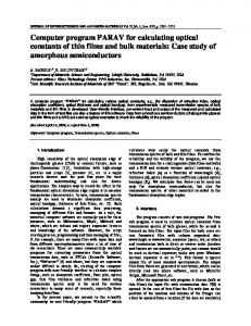
Figure (1)
illustrates the agreement between the results obtained using the algorithm presented in this paper, shown as solid curves, and the results obtained using the phenomenological model, shown as dots.
Although only the first four
harmonics are illustrated in this figure, the agreement was equally as good for higher harmonics.
22
r
0.9-
FUNDAMENTAL
1--
0.6-
-
2ND HARMONIC]
0.3
0.310
0
2
3
23 4
5
6
DISTANCE--(km )
7
t REFERENCES
1. W. Keck and R. T. Beyer, Physics of Fluids 3, 342-352 (1960).
2.
D. T. Blackstock, J. Acous. Soc. Am. 36, 534-542 (1964).
3.
K. A. Naugol'nykh, S. I. Soluyan, and R. V. Khokhlov, Soy. Phys. Acoust. 9, 42-46 (1963).
4.
B. D. Cook, J. Acous. Soc. Am. 34, 941-946 (1962).
5.
A. L. Van Buren, J. Acous. Soc. Am. 44, 1021-1027 (1968).
6.
A. L. Van Buren, J. Sound Vib.
7.
F.E. Fox and W.A. Wallace, J. Acous. Soc. Am. 26, 994-1006 (1954).
42, 273-280 (1975).
8. D. T. Blackstock, J. Acous. Soc. Am. 36, 217-219 (1964).
9.
F. B. Hildebrand, Introduction to Numerical Aanalysis (McGraw-Hill Book Company, Inc., New York, 1956).
24
I___
APPENDIX A COMPUTER PROGRAM FAW I 2 3 4 5 6 7 8 9 10
li 12 13
C C C C C C C C C C C C C
THIS PROGRAM STEPWISE CALCULATES THE HARMONIC CONTENT OF A FINITE AMPLITUDE WAVE AS A FUNCTION OF POSITION. THE INITIAL WAVEFORM MAY HAVE ANY HARMONIC CONTENT AND ARBITRARY FHASE. THE ABSORPTION COEFFICIENTS MAY BE EXTERNALLY SUPPLIED OR AN INTERNAL OMEGA SQUARED ALGORITHM IS SUPPLIED. THE INTERNAL ALGORITHM ALLOWS MODIFICATION OF ANY OF THE OMEGA SQUARED COEFFICIENTS. THE NUMERICAL INTEGRATION USES THE RUNGE-KUTTA METHOD AND THE STEP SIZE WILL AUTOMATICALLY INCREASE WHEN THE CHANGE OVER AN INTERVAL IS SMALL.
14 C 15 C 16 C 17 18 19 20 21
DIMENSION G(50),GX(50),G2(100) ,H(50),HX(50),H2(100) DIMENSION X1(50,50),XI1(50,50),X2(50,50) DIMENSION X22(50,50),XL(50),XL1(50),GH(50) DIMENSION ALPHA(50) ,DG(50),DG1(50),DH(50) ,DHI(50) DIMENSION KG(5),KH(5) DOUBLE PRECISION GGX:G2,HHXH2,X1,XllX2,X22,XLXL1 DOUBLE PRECISION GHALPHADGDG1,DHDH1,R,C,FREIBETA DOUBLE PRECISION EB,X,F1,DXRMAXRN,Z,Z1,DXIPD DOUBLE PRECISION YRO
23 24 25 26 C 27 C 28 C 29 30 31 32 33 34
~35
36 37 38 39 40 41 42 43 44 45 46 47 48 49 50 51
I
INITIALIZE REGISTERS TO ZERO DO 110 IB=1,100 G(IB)=O.DO GX(IB)=0. DO G2(IB)=O.DOH(IB)=O.D0 HX(IB)=0.D(O H2 IB)=O.DO
110
120 130 C C C C C C
CONTINUE DO 130 !C=I,50 D10 120 I1I'1, 0 . X1 ( IC, I) =0 0O XI (IC, ID)= ).10 X2(ICID)=0.l() X22(ICrD)=.DO CONTINUE CONTINUE INFUT DATA
FRE(I=FUNDAMENTAL FREQUENCY REAtI(Stl40)FREQ
____________25
-4
52 53 54 55 56
140
57
C
58 59 60 61 62 63 64 65 66 67 68 69 70 71 72 73 74 75 76 77 78 79
*80
150 C C
160 C C C
170 C C CA
180 C C C
190 C C 81 C 82 83 84 200 8s C 86 C 87 C 88 89 90 1210 91 C 92 C 93 C 94 C 9i5 96 C 97 98 220 99 10 230 101 C 102 C
FORMAT(E(17.i0)P PRINT 150YFREO FORMAT(5XYIOHFREQUENCY=PD17.10) C=SMALL SIGNAL SOUND SPEED READ'(514)C PRINT 1609C FORMAT(5XY12HSOUND SPEED=tD17.10) BETA=COEFFICIENT OF NONLINEARITY(1+B/2A) READ(5Y140)E4ETA PRINT 170,E4ETA FORMAT(5Xp5HBETAvD17#10) E=NORMALIZATION CONSTANT (OUTPUT IN D14 RE(E)) READ(59140)E PRINT 180,E FORMAT(5XY23HNORMALIZATION CONSTANT=PD17#10) DXI=INITIAL STEP SIZE READ(57140)t'XI PRINT 190tDXIA FOFMAT(5XY18HINITIAL STEP SIZE=PD17.10) RMAX=MAXIMUM PROPAGATION DISTANCE READ(',jy40)RMAX FRINr 200YRMAX FORMAT(5XY17HMAXIMUM DISTANCE=91)17.10) RO=SOURCE SIZE(INITIAL POSITION FOR GEOMETRICAL SPREADING) READ(5yl40)RO PRINT 210PIRO FORMAT(5XY12HSOURCE SIZE=vDl7#l0) A=SPREADING FACTOR =0 (PLANE WAVES) =1/2 (CYLINDRICAL WAVES) =1 (SPHERICAL WAVES) READ(59220)A FOIRMAT(F5.2) PRINT 230YA FORMAT(5Xy17HSH-'REAEIING FACTOR=PFS*.2) IAF- FLAG(AE4SORPTION COErFICIENTS)
26
103 C 104 C 105 C 106 107 240 108 109 250 110 C III C 112 C 113 114 115 260 116 C 117 C 118 C 119 C 120 121 122 123 270 124 125 280 126 C 127 C 128 C 129 130 131 290 132 C 133 C 134 C 135 136 300 137 138 310 139 C 140 C 141 C 142 143 C 144 C 145 C 146 320 147 148 330 149 150 151 C 152 340 153 C
=0 =1
(OMEGA SQUARED DEFENDENCE) (EXTERNALLY SUPPLIED)
READ(5,240)IAF FORMAT(14) PRINT 250,IAF FORMAT(5X,16HABSORPTION FLAG=?14) J=NUMBER OF HARMONICS RETAINED IN CALCULATION READ(5,240)J PRINT 260,J FORMAT(5X,2OHNUMBER OF HARMONICS=,I4) K=NUMBER OF INITIAL G COEFFICIENTS KI=NUMBER OF INIlIAL H COEFFICIENTS READ(5,240)K READ(5,240)KI PRINT 270,K FORMAT(5X,23HINITIAL 0 COEFFICIENTS=,I4) PRINi 280rKl FORMAT(5X,23HINITIAL H COEFFICIENTS=tI4) NI=NUMBER OF HARMONICS PRINTED OUT READ(5,240)NI PRINT 290,NI FORMAT(5X,27HNUMBER OF HARMONICS OUTPUT=,I4) IP-FRINT OUT INTERVAL=IP*DX READ(5,300)IP FORMAT(I8) PRINT 310,IP FORMAT(5X,19HPRINT OUT INTERVAL=,I8) OBTAIN ABSORPTION COEFFICIENTS IF(IAF) 1110,320,400 OMEGA SQUARED DEPENDENCE READ(5,140)ALPHA(1) PRINr 330,ALPHA(1) FORMAl(5X,9HALPHA(1)=,I)17.10) DO 340 IE=2,.I ALPHA(1E)=IE*IE*ALPHA(1) CONTINUE L=NUMBER OF ABSORPTION COEFFICIENTS BEING MODIFIED
27
III
154 155 156 157 158 159 160 161 162 163 164 165 166 167 168 169 170 171 172 173 174 175 176 177 178 179 180 181 182 183 184 185 186 187 188 189 190 191 192 193
C C
350 360 370
380
390 C C C 400 410
420 430 C C C 440 450 460
470 480 490
FROM OMEGA SQUARED DEPENDENCE READ(5,240)L PRINT 350,L FORMAr(5X,43HNUMBER OF MODIFIED ABSORPTION COEFFICIENTS=,I4) IF(L)1110,440,360 PRINT 370 FORMAT(5X,33HMODIFIED ABSORPTION COEFFICIENTS.) DO 390 IG=I,L READ(5,380)N,X FORMAT(14,D17.10) PRINT 380,N,X ALPHA(N)=X CONTINUE GO rO 440 INPUT ABSORPTION COEFFICIENTS PRINT 410 FORMAT(5X23HABSORPTION COEFFICIENTS) DO 430 IH=1,J READ(5,140)X ALPHA(IH)=X PRINT 420,IHALPHA(IH) FORMAT(1X,6HALPHA(,3,2H)=,D1710) CONTINUE READ INPUT WAVEFORM CONTINUE IF(k)1110t490,450 PRINT 460 FORMAT(5X,14HINPUT WAVEFORM) DO 480 IJ=lK READ(5,380)N,X G(N)=X PRINT 470,N,G(N) FORMAT(1X,2HG(,13,2H)=,D17.10) CONTINUE IF(hI)1110,530,500
194 500
DO 520 IK=1,N1
195 196 197 198 199 200 201 202 203 204
READ(5,380)N,X H(N)=X PRINT 510,N,HN) FORMAT(1X,2HH(,13,2H)=,D17.10) CONTINUE B=3.141592636*BETA*FREQ/(C*C)
510 520 530 C C C
CALCULATE MATRIX ELEMENTS DO 550 IL=2,J
28
v
V
1-7
-
205 206 207 208 209 540 210 550 211
-
-
-0 - ---
--
=
"=-
riO
213 2114 215 216 217 560 218 570 2119 220 221 580
IN1=J-IN DIO 560 IF=1,IN1 X22(INIFI=DEXF((ALPHA(IN)-ALPHA(IP)-ALPHA(IN+IP))*DXI) X2(INtIF')=1.DO CONTINUE CONTINUE DO 580 IQ=1,J GH( IQ)=DEXP(-ALPHA(IQ)*DXI) CONTINUE
C
223 224 225 226 227 228 229 230 231 232 233 234 235 236 237 238
C C
590 C C C
570 IN=1,IFX
SET COUNTER RN=RO R=RN DX=DXI PD=IP*EIX F11l.DO CB=DX*B FILL ARRAYSa DO 600 IR=1,J G2(IR)=G(IR) H2(IR)=H(IR). DG(IR)=0J0 DH(IR)=.ti0
239 600
CONTINUE
241 242 243 244 245 246 2147 248 249 250 25 1 252 253 254 255
ENTER LOOP FOR CALCULATING FIRST DERIVATIVE
C C
610 620
630
-
IL1=IL-1 DO 540 IM=1,1Ll X1 1 AILIM)=EEXPUALPHA(IL)-ALPHA(IM)-ALPHA(IL-IM))*DXI) Xl(IL,IM)- l.D0 CONTINUE CONTINUE IFX=J-1
212
222
-1-
DIO 620 IS=2,J DO 610 IT1,YIFX CX=CB*IT*X(ISYIT) DG(IS)=CX*(G2(IS-IT)*G2(IT)-H2(IS-IT)*H2(IT) )+DG(IS) DH(IS)=CX*(H2(XS-IT)*G2( IT)+G2(IS-IT)*H2(IT) )+DH( IS) CONTINUE CONTINUE DIO 640 IU=19J DO 630 IV=1,IFX CX=CB*IUI*X2(IU,IV) DG( IU)=EIG( IU)-CX*(G2( IU+IV)*G2( IV)+H2( IU+IV)*H2( IV)) E'H( IU)=DH( IU)+CX*(G2( IU+IV)*H2( IV)-H2( IU+IY)*G2( IV)) CONTINUE
29
11
-1
1 256 257 258 25 260 261
640 C C C
262 263 264 265 266 267 268 269 270 271 272 273 274 275 276 277 278 279 280 281 282 2'83 284 25 286 287 288 289 290 291 292 293 294 295 296 297 298
650 C C C
655
660 670 680 690 700 710 CJA C C C
712
714 720
299
CONTINUE CALCULATE NEW AMPLITUDES FOR SECOND DERIVATIVE DO 650 IW=I,J G2(IW)=G(IW)+DG(IW) H2(IW)=H(IW)+DH(IW) DGI(IW)=O.DO DHI(IW)=O.DO CONTINUE FIND LAST FIVE NON-ZERO HARMONICS DO 655 IW1=1,5 KG(IWI)=O KH(IW1)=O CONTINUE DO 710 IX=I,.J IF(G2(IX))660,680,660 DO 670 IY=1,4 KG(IY)=KG(IY+I) CONTINUE KG(5)=IX IF(H2(IX))690,710v690 DO 700 IZ=l,4 KH(IZ)=KH(IZ+I) CONTINUE KH(5)=IX CONTINUE
3
INSURE THAT THE LAST FIVE HARMONICS ARE NOT PROGRESSIVELY LARGER DO 720 JA=t,4 JB=KG(JA) IF(JB)712,720,712 Z=DABS(G2(JB)) JC=KG(JA+I) IF(JC)714,720,714 ZI=[ABS(G2(JC)) IF(Z1.LT.Z)GO TO 720 G2(JC)=0.95 2(.,C)*Z/ZI CONTINUE
300 301 302 722 303 304 305 724
DO 730 JD=1,4 JE::KH(JD) IF(JE)722,7309722 Z=DABS(H2(JE)) JF=KH(JD+I) IF(JF),24,p730,724 ZI=DABS(H2(JF))
306
IF(ZI.LT.Z)GO TO 730
TV
C
307
H2(JF)=0.95*H2(JF)*Z/Zl
308 730
CONTINUE
312 313
Fl=RN/R)05 CB=DX*Et*Fl
317 318 319 320 321 L322 324 325 326 327 328 329 330 331 332 333 334 335 336 337
C C C 760
ENTER LOOP FOR CALCULATING SECOND DERIVATIVE
DO 780 JG=29J DO 770 JH1,PIFX CX=CB*JH*Xll(JGYJH) 323 G1(J)=C*(62(JG-JH)*G(JH)- 2(JG-JH)*H2(JH) )+DG1(JG) D'H1(JG)=CX*(H2(JG-JH)*G2(JH)+G2(JG-JH)*H2(JH) )+DH1(JG) CONTINUEA 770 780 CONTINUE Do 800 JI=1?J DO 790 JJ1,YIFX CX=CB*JI*X22(JIYJJ) DG1(JI)=DG1UJI)-CX*(G2(JI+JJ)*G2(JJ)+H2(JI+JJ)*H2(JJ)) DH1(JI)=DH1(JI)+CX*(62(JI+JJ)*H2(JJ)-H2(JI+JJ)*02(JJ)) CONTINUE 790 CONTINUE 800 C CALCULATE NEW AMPLITUDES C C DO 810 JK=1.-J
338
G(JK)=G(JK)+O.5*(DG(JK)+DG1(JK))
339 340 810
H(JK)=H(JK)+.*(tH(J'i+DH1 (JK)) CONTINUE
341 Ct 342 343 344 345 346 347 348 349 350 351
I-352
go
C C
820
830
840 353 354 850 355 860 356 357 870
FIND LAST FIVE NON-ZERO HARMONICS DO 820 JL=1,5 KG(JL)=O KH(JL)=0 CONTINUE DO 880 JM=1,J IF(G(Jrl))830p8150?830 DO 8140 JN=1,4 KG(JN)=KG(JtI+l) CONTINUE NG(5)=JM IF(H(JM))860?880v860 DO 870 .O=1,4 KH(JO)=KH(JD+1) CONTINUE
-
--
-
-
--
t
i
358 359 360 361 362 363 364 365 366 367 368 369 370 371 372 373 374 375 376 377 378 379 380
830 C C Cm
882
884
890
892
894
2
IKH(5J)=Jh CONTINUE INSURE THAT THE LAST FIVE HARMONICS ARE NOT PROGRESSIVELY LARGER ['0 890 JF=lv4 JO=l'G(JF') IF(J0)882v890,882 Z=LAES(G(JQ))4r JR=\G (.JP+ 1 IF(JR)884,890t884 Z1DPABS(G(JR)) IF(Zl.LT.Z)GO TO 890 G(JR)=0.95*G(JR)*Z/Z1 CONTINUE [DO 900 JS=194 JT=KH(JS) IF(JT)992v900v892 Z=DABS(H(JT)) JU=I'H(JS+l) IF(JU)894,900,894m Zl=[IAES(H(JU))A IF(ZI.LT.Z)GO TO 900
381 3382 900
H(Jt))=0.95*H(JU)*Z/Zl CONTINUE
384 C
CHECK FOR OUTPUI DISTANCE
386 905 3878 388 C 389 C2= 390 910 391 392 393 394 920 395 396 397 925 398 399 930
IF((R-FRO)-PD)l0l0p95Op910
400 940
DO 94) JV1=JNI
401 402
xL(JVI)=X*G2(JV1IELIEXP(-ALPHA(JVI)fl)/E XLI(JVI)=X*H2(.JVI)*bEXP(-ALPHA(JVI)*Y)/EAl
4035 945
CONTINUE~
404 405 ?50 406 407 408 960
G0 TO 965 00 960 JX=IYNf Xl-(jX)--r1*G(JX)*(;H(JX)/E XL1 (JX)=FI*H'J)X)VGH(JX)/E CONTINUE
INTERPOLATE
S
S
m
-i
Z
OUTPUT
Y[i'X-UF:-RO)-PE') DO 920 JV=ltNI G2(JV)=c62(JV)-t'G(JV)+0.5*(ElG(JV)+DGI(JV) )*Y/DX H2(JV)=H2(JV)-iJH(JV)+0.5*(DH(JV)+DI(JV) )*Y/DJ CONTINUE X=FI IF( 1A-0.5)940.925.930 X=(RN/(RN+Y))**0.3 60 TO 940 X=R/(R(N+YT)
32
M
409 410 411 412 413 414 415 11416 *417
965 970
990
PRINT 970YPI FORMAT(5Xv9HDISTANCE=9D17.10)A PRINT 980 FORMAT('SXv3HSINp20Xt3HCOS) Do 1000 JY=1,NI PRINT 99OvJYtXL(JY)tXL1(JY) FORMAT(1X,14,4XDl7.10,5XE'17.10)
1000
CONTINUE
980
418 419 C 420 C 4 21010
CHECK STEP SIZE N=O
J )) 0 0 10
0 1 2
426 1020 427 428 1030 429 1040
Z=Z+DABS(0.5*((D'S(J1)+DlG1(J1))/G(J1))) N=N+1 IF(H(J1))104091050?1040 Z=Z+DABS(0.5*(tIH(J1)+E'H1(Jl))/H(J1))
430 431 1050
N=N+1 CONTINUE
433 434 436 437 438 439 440 441 442 443 444
MODIFY WAVEFORM
C C
1060 C C C
[i445
446 1070 447 448
II450 9449
FIJ=PD+IP*DXI GO TO 905
451 1080 452 1090 45-3 454 1106
I458
G(J2)=G(J2)*F1*GH(J2) H(J2)=H(J2)*F1*GH(J2) CONTINUE IF(Z.GT.(N*0.005))GO TO 1100 DOUBLE STEP SIZE DX=2.0*DX DO 1070 J2=1,J
GH(J2))=GH(J2)*GH(J2) CONTINUE DO 1090 J31vtJ DO 1080 J4=1 9 J X11(J3,J4)=X1I(J3 7-J4)*X11 (J3,J4)
X22(J3,J4)=X-2( J31 J4)*X22(J3,J4) CONTINUE CONTINUE PRIUT 11069DX FORMAT(1Xt3HDX=9Dl7o10)
455 1100
RN=R
457 1110
STO)P
END
APPENDIX B SAMPLE OUTPUT FROM FAW
FREQUENCY= 0.3000000000D 03 SOUND SPEED= 0.1500000000D 04 BETA= 0.3500000000D 01 NORMALIZATION CONSTANT= 0.6670000000D-01 INITIAL STEP SIZE= 0.1000000000D 02 MAXIMUM DISTANCE= 0.1000000000D 05 SOURCE SIZE= O.OOOOOOOOOOD 00 SPREADING FACTOR= 0.00 ABSORPTION FLAG= 0 NUMBER OF HARMONICS= 40 INITIAL G COEFFICIENTS= 1 INITIAL H COEFFICIENTS= 0 NUMBER OF HARMONICS OUTPUT= 5 PRINT OUT INTERVAL= 100 ALPHA(1)= 0.1120000000D-05 NUMBER OF MODIFIED ABSORPTION COEFFICIENTS= INPUT WAVEFORM G( 1)= 0.6670000000D-01 DISTANCE= 0.1000000000D 04 SIN COS 1 0.9941231144D 00 0.0000000000D 00 2 0.9622622120D-01 0.00000000001 00 0.0000000000D 00 3 0.1394984526D-01 4 0.2394449333D-02 0.O000000000D 00 J 0.4511965196D-03 O.00000000011 00 DISTANCE= 0.2000000000D 04 COS SIN 1 0.9788882494D 00 O.000000000D 00 2 0.1845999987D 00 .000000000)D 00 3 0.5197039094D-01 .000000000)D 00 4 0.1729678606D--01 0.0000000000D 00 5 0.6313700593D-02 .000000000)D 00 DISTANCE= 0.3000000000D 04 SIN COS 1 0.9546672934D 00 .000000000)D 00 2 3 4
0.2587699767D 00 0,1041698315D 00 0.4945203382D-01 0.15709949110-01 DX= 0.2000000000D 02 DISTANCE= 0.4000000000D 04 SIN Cos 1 0.9220214992D 00 2 0.3138414940D 00 3 0*1574155764D 00 0.9275848905D-01
O.000000000D 0.O000000000D 0.OOOOOOOOOO1 0.00000000001
5 0.5972644773D-01 DX= 0.4000000000D 02
0.00000000001
!v!
00 00 00 00
.000000000)D 00 O.0000000000 00 0000000000D 00 0.0000000000)000 00
i 0
DISTANCE=
0.5000000000
SIN
04
COS
1 2 3 4 5
0.8817469738D 00 0.34690482481D 00 0.1988133777D 00 0.13306357721D 00 0.9695954537D-01 DX= 0.3000000000D, 02 DISTANCE= 0.6000j00000D 04 SIN Cos 1 0.8353073629D 00 2 0.3581480161D 00 3 0.22020568081) 00 4 0.1567515441D 00 5 0.1208128685D 00 DX= 0.1600000000P 03 DISTANCE= 0.7000000000D 04 SIN
1 2
0.78636354951D 00 0.3538678457D 00
0.O000000000D O.O000000000D 0.00000000000D 0.00000000001) 0.00000000001
00 0 00 00 00 00
COS O.O000000000D 00 0.0000000000D 00
3 4 5
0.2247481885'D 0.1638955398[ 00 0.12878692231D 00 00 DX= 0.3200000000D' 03 DISTANCE= 0.8000000000D 04 SIN COS 1 0.738935130211 00 2 0.34231987871D 00 3 0.22103348636D 00 4 0.16292265481D 00 5 0.1290571601D 00 DISTANCE= 0.9000000000D 04 SIN COS I 0.694735733D 00 2 0.32794109021) 00 3 0.2137387066D 00 4 0.1583862311D 00 5 0.1259628330D 00 DISTANCE= 0.1000000000D' 05 SIN Cos 1 0.6542737913D' 00 0.3128153020D' 00 3 0.2050573568P' 00 4 0.1523-8922581) 00 5
O.O000000000D 00 O.c'OOOOO0D O00 O.O000000000D 00 0.00000000001) 00 O.O000000000D 00
0.1214645359D 00
0.000000000011 00
0.00000000001) 00 O.O000000000D 00
0.0000000000D 0.0000000000D 0.000000000D 0.0000000000D O.O000000000D
00 00 00 00 00
I O.O000000000D 0.0000000000' 0 0000000000 O.O000000000D0 0.0000000000D
00 00 00 00 00
0,00000000001' 0.00000000001' 0.oooooooooo1) 0.0000000000'
00 00 00 00
0.00000000001' 00
35
I