mining, support is defined over the binary domain. {0, 1}, where 1 indicates the presence of an item in a transaction, and 0 its absence. The share measure [2] ...
A Foundational Approach to Mining Itemset Utilities from Databases Hong Yao, Howard J. Hamilton, and Cory J. Butz Department of Computer Science University of Regina Regina, SK, Canada, S4S 0A2 {yao2hong, hamilton, butz}@cs.uregina.ca Abstract Most approaches to mining association rules implicitly consider the utilities of the itemsets to be equal. We assume that the utilities of itemsets may differ, and identify the high utility itemsets based on information in the transaction database and external information about utilities. Our theoretical analysis of the resulting problem lays the foundation for future utility mining algorithms.
1
Introduction
We describe utility mining, which finds all itemsets in a transaction database with utility values higher than the minutil threshold. Standard methods for mining association rules [1, 7] are based on the supportconfidence model. They first find all frequent itemsets, i.e., itemsets with support of at least minsup, and then, from these itemsets, generate all association rules with confidence of at least minconf. The support measure is used because it is assumed that only highly frequent itemsets are likely to be of interest to users. The frequency of an itemset may not be a sufficient indicator of interestingness, because it only reflects the number of transactions in the database that contain the itemset. It does not reveal the utility of an itemset, which can be measured in terms of cost, profit, or other expressions of user preference. For example, the small transaction database shown in Figure 1 indicates the quantity sold of each item in each transaction. This information is of high utility. In association rule mining, support is defined over the binary domain {0, 1}, where 1 indicates the presence of an item in a transaction, and 0 its absence. The share measure [2] was proposed to overcome the shortcomings of support. It reflects the impact of the quantity sold on the cost or profit of an itemset. Lu et al. proposed a scheme for weighting each item using a constant value without regard to the significance of transactions [5]. In their scheme, the utilities are attached to the the items rather than the transactions. Wang et al. [9] suggested that it remains unclear
TID T1 T2 T3 T4 T5 T6 T7 T8 T9 T10
Item A 1 0 1 0 0 0 0 4 0 0
Item B 0 0 0 0 0 0 0 0 1 0
Item C 1 6 2 4 3 1 8 0 1 0
Item D 14 0 4 0 1 13 0 7 10 18
Figure 1: An Example Transaction Database
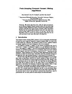
to what extent patterns can be used to maximize the business profit for an enterprise. For example, two association rules {Perfume} −→ Lipstick and {Perfume} −→ Diamond may suggest different utilities to a sales manager, although both are interesting rules. They assume that the same item can have several utility functions with corresponding profit margins. The goal for profit mining is to recommend a reasonable utility function for selling target items in the future. Chan et al. [3] recently described an alternate approach to mining high utility itemsets. In this paper, we generalize previous work on itemset share [2]. We define two types of utilities for items, transaction utility and external utility. The transaction utility of an item in a transaction is defined according to the information stored in the transaction. For example, the quantity of an item sold in the transaction might be used as the transaction utility. The external utility of an item is based on information not available in the transaction. For example, it might be stored in a utility table, such as that shown in Figure 2, which indicates the maximum profit for each item. The external utility is proposed as a new measure for describing user preferences. By processing a transaction database and a utility
Item Name Item A Item B Item C Item D
Profit($) 3 150 10 1
Figure 2: An Example Utility Table
table together, data mining can be guided by the utilities of itemsets. The discovered knowledge may be useful for maximizing a user’s goal. For example, if the goal of a supermarket manager is to maximize profit, the itemset utilities should be decided by the quantity of items sold and the unit profit on these items. The quantity sold is a transaction utility, and the unit profit is a external utility. The discovered knowledge is the itemsets that produce the largest profits. The reminder of the paper is organized as follows. In Section 2, the problem of utility mining is stated. In Section 3, we propose a theoretical model for our utility mining approach. In Section 4, conclusions are stated.
to be scaled or normalized to correctly reflect the transaction utility of items. For example, if the items represent temperatures, we cannot simply say that the transaction utility of item A is six times that of item B because o(A) = 6 and o(B) = 1. For simplicity, we ignore the required transformations in this paper. Definition 2.3. The external utility value of an item is a numerical value s(iq ) associated with an item iq such that s(iq ) = U (iq ), where U is a utility function, a function relating specific values in a domain to user preferences. The external utility reflects the utility per item that is independent of transaction. Figure 2 shows profit values, e.g., s(A) = 3 and s(B) = 150. It reveals that the supermarket can earn $3 for each item A that is sold. Often, in practice, it is feasible and more convenient to specify the utility function by roster as a utility table. Definition 2.4. (Utility Table). A utility table is a two dimensional table UT�I, U � over a collection of items I = �i1 , i2 , . . . im �, where U is the set of real numbers such that s(iq ) = U (iq ) for each iq ∈ I.
In this section, a formal description of the problem of utility mining is given and related concepts are described. The utility mining problem is defined as follows.
Before defining the utility value of an item, the utility function needs to be defined. Piatetsky-Shapiro et al. [8] and Kl¨ osgen [4] suggested that a quantitative measure of a rule may be computed as a function and introduced axioms for such quantitative measures. We define a utility function based on their axioms.
Definition 2.1. (Utility Mining). Let I = {i1 , i2 , . . . im } be a set of items, D be a transaction database, and UT�I, U � be a utility table, where U is a subset of the real numbers that reflect the utilities of the items. The utility mining problem is to discover all itemsets in a transaction database D with utility values higher than the minutil threshold, given a utility table UT .
Definition 2.5. A utility function f (o, s) is a two variable function, that satisfies: (1) f (o, s) monotonically increases in f (o, s) for fixed o. (2) f (o, s) monotonically increases in f (o, s) for fixed s.
2
Statement of Problem
According to the above problem statement, we need to describe and define the utility of an item and an itemset. In the remainder of this section, we first define the utility of an item and then give the definition of the utility of an itemset. We also extend definitions from [2] to define transaction utility. Definition 2.2. The transaction utility value in a transaction, denoted o(ip , Tq ), is the value of an item ip in a transaction Tq . The transaction utility reflects the utility in a transaction database. The quantity sold values in Figure 1 are the transaction utility values of the items in each transaction. For example, o(D, T1 ) = 14. In general, a transaction utility value may need
The utility value of an item is defined as follows. Definition 2.6. The utility of an item iq in a transaction Tq , denoted u(iq , Tq ), is f (o(iq , Tq ), s(iq )), where o(iq , Tq ) is the transaction utility value of iq , s(iq ) is the external utility value of iq , and f is a utility function. The utility of an item can be an integer value, such as the quantity sold, or a real value, such as a profit margin, total revenue, or unit cost. Example 2.1. Given the transaction database in Figure 1, the utility table in Figure 2, and utility function f (o(iq , Tq ), s(iq )) = Amount × Item Profit, we obtain u(A, T1 ) = 1 × 3 = 3. The supermarket earns $3 by selling one item A in transaction T1 . Similarly, u(B, T1 ) = 0, u(C, T1 ) = 10, and u(D, T1 ) = 14.
Example 2.1 shows that the utility of a item depends on the external item utility and the transaction utility as well as the frequency. The utility of item D, a frequent item sold 67 times in total, is less than the utility of item B, an infrequent item sold only once. Association rule mining approaches based on the support measure could miss such high utility items. The utility of an itemset is defined according the sum of the utilities of its items.
In this section, we describe two important properties of utility that allow an upper bound on the utility of a k−itemset to be calculated from the utilities of the discovered (k − 1)−itemsets. Furthermore, a heuristic model for estimating itemset utility is proposed that prunes the search space by predicting whether itemsets should be counted. These results provide the theoretical foundation for efficient algorithms for utility mining.
Definition 2.7. [2] A k−itemset is an itemset, X = {x1 , x2 , . . . , xk }, X ⊆ I, 1 ≤ k ≤ m, of k distinct items. Each itemset X has an associated set of transactions TX = {T q ∈ D|Tq ⊇ X}, which is the set of transactions that contain itemset X.
= Definition 3.1. Given a k−itemset I k k = I − {i {i1 , i2 , . . . ik } and ip ∈ I k , we define Iik−1 p} p as the (k − 1)−itemset that includes all items in I k except item ip .
Definition 2.8. The local utility of an item xi in an itemset X, denoted l(xi , X), is the sum of the utilities of the item xi in all transactions containing X, i.e., � l(xi , X) = (2.1) u(xi , Tq ). Tq ∈TX
For example, using the transaction database in Figure 1 and the utility table in Figure 2, l(A, ACD) = 2×3 = 6. Definition 2.9. The utility of an itemset X, denoted u(X), is the sum of the local utilities of each item in X in all transactions containing X, i.e., (2.2)
u(X) =
k �
l(xi , X).
i=1
If f (o(iq , Tq ), s(iq )) = Amount × Item Profit, then for itemset ACD, u(ACD) = l(A, ACD) + l(C, ACD) + l(D, ACD) = 2 × 3 + 3 × 10 + 18 × 1 = 54. 3 Theoretical Model of Utility Mining A key property of itemsets is the Apriori property (or downward closure property) [1, 7], which states that if an itemset is frequent by support, then all its subsets must also be frequent by support. It guarantees that the set of frequent itemsets is downward closed with respect to the lattice of all its subsets [2]. This closure property has permitted the development of efficient algorithms that traverse only a portion of the itemset lattice. However, when calculating the utility of an itemset, the itemset utility can increase or decrease as the itemset is extended by adding items. For example, u(A) = 3 × 6 = 18 but u(AD) = 43 > u(A), u(B) = 1 × 150 = 150 but u(AB) = 0 < u(B). Thus, itemset utility does not satisfy downward closure, and it is necessary to discover other properties of itemset utility to enable the design of efficient algorithms.
3 For the 4-itemset I 4 = {A, B, C, D}, we have IA = 3 3 {B, C, D}, IB = {A, C, D}, IC = {A, B, D}, and 3 ID = {A, B, C}.
Definition 3.2. Given a k-itemset Ik = k−1 k−1 k−1 {i1 , i2 , . . . ik }, we define S = {Ii1 , Ii2 , . . . , Iik−1 } k as the set of all (k − 1)−subsets of I k . For the 4-itemset I 4 = {A, B, C, D}, we have S 3 = {BCD, ACD, ABD, ABC}. Lemma 3.1. The cardinality of S k−1 , denoted |S k−1 |, is k. Lemma 3.1 indicates that the number of the subsets of size (k − 1) of I k is k. Definition 3.3. Let I k = {i1 , i2 , . . . ik } be a kitemset, and let S k−1 be the set of all subsets of I k of size (k − 1). For a given item ip , the set Sik−1 p = {I k−1 |ip ∈ I k−1 and I k−1 ∈ S k−1 } is the set of (k − 1)−itemsets that each includes ip . 3 For the 4-itemset I 4 = {A, B, C, D}, we have SA = 3 / BCD. {ACD, ABD, ABC}. BCD ∈ / SA because A ∈
Lemma 3.2. The cardinality of Sik−1 , denoted |Sik−1 |, p p is k − 1. Lemma 3.2 indicates that among the k subsets of I k of size (k − 1), there are (k − 1) subsets that include item ip and only one that does not. Theorem 3.1. Given a k-itemset I k = {i1 , i2 , . . . ik } and a (k − 1)−itemset I k−1 such that I k−1 ⊂ I k , then ∀ ip ∈ I k−1 , l(ip , I k ) ≤ l(ip , I k−1 ). Proof: since I k−1 is a subset of I k , any transaction Tq ∈ TI k must satisfy Tq ∈ TI k−1 . Thus, according to Equation 2.1 in Definition 2.8, l(ip , I k ) ≤ l(ip , I k−1 ) holds. For the 4-itemset I 4 = {A, B, C, D} in Figure 1 and the utility table in Figure 2, we have a 3-itemset ACD and a 2-itemset AD, and AD ⊂ ACD. Here,
l(A, ACD) = 2 × 3 = 6, l(A, AD) = 6 × 3 = 18, and thus l(A, ACD) ≤ l(A, AD). Theorem 3.1 indicates that the local utility value of an item ip in an itemset I must be less than or equal to the local utility value of the item ip in any subset of I that includes item ip . Using Lemma 3.2 and Theorem 3.1, we obtain Theorem 3.2. Theorem 3.2. The local utility of an item ip in an itemset I must be less than or equal to the local utility of item ip in any subset of I of size (k − 1). Formally, local utility satisfies (3.3) (3.4)
Example 3.1. For a 4-itemset I 4 = {A, B, C, D}, we have l(A, I 4 ) ≤ min{l(A, ABC), l(A, ABD), l(A, ACD)} l(A, ABC) + l(A, ABD) + l(A, ACD) ≤ 3
Theorem 3.2 allows the calculation of an upper bound for the utility of an item in a k−itemset I by calculating the utilities of subsets of I of size (k − 1). Using Theorem 3.2, an upper bound for the utility of an itemset can also be inferred. Theorem 3.3. (Utility Bound Property). utility of an k−itemset I k must satisfy �k
u(ABC) + u(ACD) + u(ABD) + u(BCD) 3
Although the utility bound property limits the utility of a k−itemset I to a fraction of the sum of the utilities of all subsets of size (k − 1), the upper bound is still high. Thus, we further reduce this bound by considering the support of the itemset, denoted sup(I), the percentage of all transactions that contain the itemset [1, 7].
(3.6)
Proof: According to Theorem 3.1, the first inequality holds. According to Lemma 3.2, there are (k − 1) subsets of size (k − 1). By substituting each l(ip , I k−1 ) into minI k−1 ∈S k−1 {l(ip , I k−1 )}, the second inequality can be shown.
u(I k ) ≤
u(I 4 ) ≤
Theorem 3.4. (Support Bound Property). If is a I k = {i1 , i2 , . . . ik } is a k−itemset and Iik−1 p k−1 k (k − 1)−itemset such that Iip = I − {ip }, where ip ∈ I k , then they satisfy
l(ip , I k ) ≤ min {l(ip , I k−1 )} I k−1 ∈S k−1 � k−1 ) k−1 k−1 l(ip , I ≤ I ∈S k−1
where ip ∈ I k−1 .
(3.5)
Example 3.2. For a 4-itemset I 4 = {A, B, C, D}, we have
The
u(Iik−1 ) k−1
i=1
Proof: Since Equation 3.4 holds for each ip ∈ I. According to Equation 2.1, Equation 3.5 is obtained. Theorem 3.3 indicates that the upper bound of the k−itemset utility is limited by the utilities of all its subsets of size (k − 1). Thus, a level-wise method, such as that provided by Mannila et al. [6], can be used to prune itemsets with utilities less than a threshold. As a result, the search space can be reduced.
sup(I k ) ≤
min {sup(Iik−1 )} p
∀Iik−1 ⊂I k p
Proof: Since Iik−1 is a subset of I k , any transaction p Tq ∈ TI k must satisfy Tq ∈ TI k−1 . Thus, according to ip
) holds. the definition of support, sup(I k ) ≤ sup(Iik−1 p Theorem 3.4 indicates that the support of an itemset always decreases as its size increases. Theorem 3.4 also indicates that if the support of an itemset is zero, then the support of any superset of the itemset is also zero. That is to say that if sup(I k−1 ) = 0 and I k−1 ⊂ I k then sup(I k ) = 0. For example, for the 4-itemset I 4 = {A, B, C, D} in Figure 1, sup(ABCD) is less than or equal to min{sup(ABC), sup(ABD), sup(ACD), sup(BCD)}. Based on the utility bound property and the support bound property, a heuristic model to predict the expected utility value of a k−itemset I k , denoted u� (I k ), is given as follows.
(3.7)
u� (I k ) =
k
supmin � u(Iik−1 ) k − 1 i=1 sup(Iik−1 )
where (3.8)
supmin =
)} min {sup(Iik−1 p
∀Iik−1 ⊂I k p
Since the support bound property only allows us to estimate the number of transactions, Equation 3.7 may sacrifice some accuracy, and thus our proposed model is a heuristic model.
Example 3.3. For the 3-itemset I 3 = {B, C, D} in Figure 1 and the utility table in Figure 2, we have supmin = min{sup(BC), sup(BD), sup(CD)} = min{0.1, 0.1, 0.5} = 0.1 and u� (BCD) =
supmin 3−1
u(BC) × ( sup(BC) +
=
0.1 2
× ( 150+10 + 0.1
150+10 0.1
=
0.1 2
× ( 160 0.1 +
+
160 0.1
+
122 0.5 )
u(BD) sup(BD)
+
u(CD) sup(CD) )
24+24+31+23+20 ) 0.5
= 172.2
We can directly obtain u(BCD) = 1 × 150 + 1 × 10 + 10 × 1 = 170 from Figure 1 and Figure 2. Equation 3.7 requires that the utilities of all subsets of size (k − 1) take part in calculation, which leads to inefficiencies in algorithms. Next, we relax this constraint. Definition 3.4. If I is an itemset with utility u(I) such that u(I) ≥ minutil, where minutil is the utility threshold, then itemset I is called a high utility itemset; otherwise I is called a low utility itemset. The following theorem guarantees that only the high utility itemsets at level (k − 1) are required to estimate the utility of a k−itemset. Theorem 3.5. Let u� (I k ) be the expected utility of I k as described in Equation 3.7, and let u(I1k−1 ), u(I2k−1 ), . . . u(Ikk−1 ) be the k utility values of all subsets of I k of size (k − 1). Suppose, Iik−1 (1 ≤ i ≤ m) are high utility itemsets, and Iik−1 (m + 1 < i ≤ k) are low utility itemsets. Then u� (I k ) ≤
m supmin� � u(Iik−1 ) k−m × minutil + k − 1 i=1 sup(Iik−1 ) k−1
where (3.9) supmin� =
min
Iik−1 ⊂I k ,(1≤i≤m)
{sup(Iik−1 )}
Proof: since u(Iik−1 ) ≤ minutil when m+1 < i ≤ k, we can substitute minutil for each u(Iik−1 ) term (m + 1 < i ≤ k) in Equation 3.7, obtaining the desired result. Example 3.4. For the 3-itemset I 3 = {B, C, D} in Figure 1 and the the utility table in Figure 2, suppose minutil = 130. Since u(CD) = 122 < minutil, then supmin� = min{sup(BC), sup(BD)} = min{0.1, 0.1} = 0.1. The estimated utility of BCD is calculated as follows u� (BCD) ≤
u(BC) supmin� 3−1 ( sup(BC)
+
u(BD) 3−2 sup(BD) ) + 3−1 minutil
=
0.1 2
× ( 150+10 0.1 ) +
150+10 0.1 )
=
0.1 2
× ( 160 0.1 +
+
160 0.1 )
1 2
+
1 2
× 130
× 130 = 225
Theorem 3.5 is the mathematical model of utility mining that we will use to design an algorithm to estimate the expected utility of a k−itemset from the known utilities of its high utility itemsets of size (k−1). 4
Conclusions
In this paper, we defined the problem of utility mining. By analyzing the utility relationships among itemsets, we identified the utility bound property and the support bound property. Furthermore, we defined the mathematical model of utility mining based on these properties. In the future, we will design an algorithm and compare it to other itemset mining algorithms. References [1] R. Agrawal, T. Imielinski, and A. N. Swami. Mining association rules between sets of items in large databases. In Proceedings of the 1993 ACM SIGMOD International Conference on Management of Data, pages 207–216, Washington, USA, 1993. [2] B. Barber and H.J. Hamilton. Extracting share frequent itemsets with infrequent subsets. Data Mining and Knowledge Discovery, 7(2):153–185, 2003. [3] R. Chan, Q. Yang, and Y.-D. Shen, Mining high utility itemsets. In Proceedings of the 2003 IEEE International Conference on Data Mining (ICDM 2003), pages 19–26, Melbourne, FL, November 2003. [4] W. Klosgen. Explora: a multipattern and multistrategy discovery assistant. In U.M Fayyad, G. PiatetskyShapiro, P. Smyth, and R. Uthurusamy, editors, Advances in Knowledge Discovery and Data Mining, pages 249–271. AAAI/MIT Press, 1996. [5] S. Lu, H. Hu, and F. Li. Mining weighted association rules. Intelligent Data Analysis, 5(3):211–225, 2001. [6] H. Mannila and H. Toivonen. Levelwise search and borders of theories in knowledge discovery. Data Mining and Knowledge Discovery, 1(3):241–258, 1997. [7] H. Mannila, H. Toivonen, and A.I. Verkamo. Efficient algorithms for discovering association rules. In AAAI Workshop on Knowledge Discovery in Databases (KDD’94), pages 181–192, Seattle, Washington, July 1994. AAAI Press. [8] G. Piatetsky-Shapiro. Discovery, analysis and presentation of strong rules. In G. Piatetsky-Shapiro and W.J. Frawley, editors, Knowledge Discovery in Databases, pages 229–248. AAAI/MIT Press, 1991. [9] K. Wang, S. Q. Zhou, and J. W. Han. Profit mining: From patterns to actions. In Advances in Database Technology, 8th International Conference on Extending Database Technology (EDBT’2002), pages 70–87, Prague, Czech Republic, 2002. Springer.