ZART: A Multifunctional Itemset Mining Algorithm - CiteSeerX

ZART: A Multifunctional Itemset Mining Algorithm Laszlo Szathmary1 , Amedeo Napoli1 , and Sergei O. Kuznetsov2 1

LORIA UMR 7503, B.P. 239, 54506 Vandœuvre-lès-Nancy Cedex, France {szathmar, napoli}@loria.fr 2 Higher School of Economics, Department of Applied Mathematics Kirpichnaya 33/5, Moscow 105679, Russia [email protected]

Abstract. In this paper3 , we present platform Coron, which is a domain independent, multi-purposed data mining platform, incorporating a rich collection of data mining algorithms. One of these algorithms is a multifunctional itemset mining algorithm called Zart, which is based on the Pascal algorithm, with some additional features. In particular, Zart is able to perform the following, usually independent, tasks: identify frequent closed itemsets and associate generators to their closures. This allows one to find minimal non-redundant association rules. At present, Coron appears to be an original working platform, integrating efficient algorithms for both itemset and association rule extraction, allowing a number of auxiliary operations for preparing and filtering data, and, for interpreting the extracted units of knowledge.

1

Introduction

Finding association rules is one of the most important tasks in data mining today. Generating strong association rules from frequent itemsets often results in a huge number of rules, which limits their usefulness in real life applications. To solve this problem, different concise representations of association rules have been proposed, e.g. generic basis (GB), informative basis (IB) [1], representative rules (RR) [2], Duquennes-Guigues basis (DG) [3], Luxenburger basis (LB) [4], proper basis (PB), structural basis (SB) [5], etc. A very good comparative study of these bases can be found in [6], where it is stated that a rule representation should be lossless (should enable derivation of all strong rules), sound (should forbid derivation of rules that are not strong) and informative (should allow determination of rules parameters such as support and confidence). M. Kryszkiewicz has shown in [6] that minimal non-redundant rules4 (MN R) with the cover operator, and transitive reduction of minimal non-redundant rules4 (RMN R) with the cover operator and the confidence transitivity property are lossless, sound and informative representations of all strong association 3 4

Reference ID of this research report: http://hal.inria.fr/inria-00001271 . Defined in Section 2.

2

Laszlo Szathmary et al.

rules. From the definitions of MN R and RMN R it can be seen that we only need frequent closed itemsets and their generators to produce these rules. Frequent itemsets have several condensed representations, e.g. closed itemsets [7– 10], generator representation [11, 12], approximate free-sets [13], disjunction-free sets [14], disjunction-free generators [11], generalized disjunction-free generators [15] and non-derivable itemsets [16, 17]. However, from the application point of view, the most useful representations are frequent closed itemsets and frequent generators that proved to be useful not only in the case of representative and non-redundant association rules, but as well as representative episode rules [18], which constitute concise, lossless representations of all association/episode rules of interest. Common feature of these rule representations is that only closed itemsets and generators are involved. 1.1

Contribution and Motivation

In our present work we are interested to find minimal non-redundant association rules (MN R) because of two reasons. First, these rules are lossless, sound and informative [6]. Secondly, among rules with the same support and same confidence, these rules contain the most information and these rules can be the most useful in practice [19]. The minimal non-redundant association rules were introduced in [1]. In [12] and [20] Bastide et al. presented Pascal, and claimed that MN R can be extracted with this algorithm. We do not agree with them because of two reasons. First, frequent closed itemsets must also be known. Secondly, frequent generators must be associated to their closures. Figure 1 shows what information is provided by Pascal when executed on dataset D5 (Tab. 3), i.e. it finds frequent itemsets and marks frequent generators. Looking at the definitions of MN R and RMN R, clearly, this information is insufficient. However, with an extension, Pascal can be enriched to fulfill the previous two criteria. This is the so-called Zart algorithm, whose result is shown in Fig. 1 on the right side. Obviously, this result is necessary and sufficient to generate GB, IB, RIB, MN R and RMN R.6 We have chosen Pascal because of the following reasons. First, among levelwise frequent itemset miner algorithms it may be the most efficient thanks to its pattern counting inference mechanism. Pascal also constructs frequent generators. As a consequence, Pascal may be a good basis for constructing closed itemsets and their generators. 1.2

Short Overview of Zart

Zart is a levelwise algorithm that enumerates candidate itemsets in ascending order by their size. It means that the generators of a class are found first. Their support is calculated, and later when finding other (larger) elements of the class, 5 6

Throughout the paper we will use this dataset for our examples. Defined in Section 2.

ZART: A Multifunctional Itemset Mining Algorithm

ABCE 2

ABC AC

3

AB

2

2

ABCE

ACE

BC

AE

A

ABC 3

BCE 3

3

2

3

ABE

3

CE

BE

3

BCE

3

ABE

3

BC

CE

AE

4 4

4

B

ACE

3

AC AB

4

3

4

C

BE

4

4

A

E

B

4

E C

BE

equivalence class

frequent itemset (FI)

(direct) neighbors

BE frequent closed itemset

B

frequent generator (FG)

B

frequent generator

transitive relation

Fig. 1. Result of Pascal (left) and Zart (right) on D with min supp = 2 (40%)

their support does not have to be counted since it is equal to the support of the generators that are already known. Apriori has a serious drawback: it has to count the support of each candidate itemset, and it necessitates one whole database pass at each iteration. Due to the counting inference support the number of expensive database passes and support counts can be reduced seriously, especially in the case of dense, highly correlated data. Shortly, Zart works the following way: as it is based on Pascal, first it finds frequent itemsets and marks frequent generators. Then, it filters frequent closed itemsets among frequent itemsets, like Apriori-Close [5]. The idea is that an itemset is not closed if it has a superset with the same support. Thus, if at the ith iteration an itemset has a subset of size (i − 1) with the same support, then the subset is not a closed itemset. This way all frequent closed itemsets can be found. The last step consists in associating generators to their closures. This can be done by collecting the non-closed generator subsets of the given closed itemset that have the same support.

2

Basic Concepts

Below we use standard definitions of Data Mining. We consider a set of objects O = {o1 , o2 , . . . , om }, a set of attributes A = {a1 , a2 , . . . , an }, and a relation R ⊆ O × A, where R(o, a) means that the object o has the attribute a. In formal concept analysis [21] the triple (O, A, R) is called a formal context. A set of items is called an itemset or a pattern. An itemset of size i is called an i-long itemset, or simply an i-itemset.7 We say that an itemset P ⊆ A is included in an object 7

For instance, {ABE} is a 3-itemset.

4


o ∈ O, if (o, p) ∈ R for all p ∈ P . The support of an itemset P indicates how many objects include the itemset. An itemset P is called frequent , if its support is not less than a given minimum support (below often denoted by min supp), i.e. supp(P ) ≥ min supp. An itemset X is called closed if there exists no proper superset Y (X ⊂ Y ) with the same support. The task of frequent itemset mining consists of generating all (closed) itemsets (with their supports) with supports greater than or equal to a specified min supp. An association rule is an expression of the form I1 → I2 , where I1 and I2 are arbitrary itemsets (I1 , I2 ∈ A), I1 ∩ I2 = ∅ and I2 6= ∅. The left side, I1 is called antecedent, the right side, I2 is called consequent. The support of an association rule8 r is defined as: supp(r) = supp(I1 ∪ I2 ). The confidence of an association rule r: I1 → I2 is defined as the conditional probability that an object includes I2 , given that it includes I1 : conf (r) = supp(I1 ∪ I2 )/supp(I1 ). An association rule r with conf (r) = 100% is called an exact association rule. If conf (r) < 100%, then r is called an approximate association rule. An association rule is strong (their set is denoted by AR) if its support and confidence are not less than the user-defined thresholds min supp and min conf, respectively. The problem of mining association rules in a database D consists of finding all strong rules in the database. This problem is usually reduced to the problem of mining frequent (closed) itemsets. Definition 1 (generic basis for exact association rules). Let F C be the set of frequent closed itemsets. For each frequent closed itemset f, let F Gf denote the set of frequent generators9 of f. The generic basis for exact association rules: GB = {r : g ⇒ (f \g) | f ∈ F C ∧ g ∈ F Gf ∧ g 6= f }. Definition 2 (informative basis for approximate association rules). Let F C be the set of frequent closed itemsets and let F G denote the set of frequent generators9 . The notation γ(g) signifies the closure of itemset g. The informative basis: IB = {r : g → (f \g) | f ∈ F C ∧ g ∈ F G ∧ γ(g) ⊂ f }. Definition 3 (transitive reduction of the informative basis). Let IB the informative basis for approximate association rules, and let F C denote the set of frequent closed itemsets. The transitive reduction of the informative basis: RIB = {r : g → (f \g) ∈ IB | γ(g) is a maximal proper subset of f in F C}. Definition 4. Minimal non-redundant rules (MN R) are defined as: MN R = GB ∪ IB. Definition 5. Transitive reduction of minimal non-redundant rules (RMN R) is defined as: RMN R = GB ∪ RIB. Clearly, RIB ⊆ IB, RMN R ⊆ MN R, GB ⊆ RMN R ⊆ MN R, IB ⊆ MN R and RIB ⊆ RMN R. 8

9

In this paper we use absolute values, but the support of an association rule r is also often defined as supp(r) = supp(I1 ∪ I2 )/|O|. See Def. 7 in Section 3.


3

5

Main Characteristics of Zart

Zart has three main features, namely 1) pattern counting inference, 2) identifying frequent closed itemsets, and 3) identifying generators of frequent closed itemsets. In this section we give the theoretical basis of Zart. 3.1

Pattern Counting Inference

The first part of Zart is based on Pascal, thus the definitions of this paragraph mainly rely on [12], where one can also find the proofs of Prop(s). 1, 2 and Th(s). 1, 2. Pascal introduced pattern counting inference, which is based on the following observation. Frequent itemsets in a database are not completely independent one from another. Itemsets that are common to the same set of objects belong to the same equivalence class. In a class three kinds of elements are distinguished: the maximal element, the minimal element(s) (wrt. set inclusion), and all other elements. The maximal element is the closure of all the elements in the class, thus it is a frequent closed itemset. The minimal elements are called generators. They are the smallest subsets of the closure of the class. A class has the special property that all its elements have exactly the same support. This is the key idea behind the counting inference. Levelwise algorithms are based on two basic properties of Apriori, namely downward closure (all subsets of a frequent itemset are frequent) and antimonotonicity (all supersets of an infrequent itemset are infrequent). Like Apriori or Pascal, Zart traverses the powerset lattice of a database in a levelwise manner. At the ith iteration, the algorithm first generates candidate i-long itemsets. Using the Apriori properties, only the potentially frequent candidates are kept, i.e. those whose (i−1)-long subsets are all frequent. After this, with one database pass the support of all candidate i-long itemsets can be determined. Pattern counting inference is based on the observation that frequent itemsets can be grouped in classes. All itemsets in a class are equivalent, in the sense that they describe exactly the same set of objects: Definition 6 (equivalence class). Let f be the function that assigns to each itemset P ⊆ A the set of all objects that include P : f (P ) = {o ∈ O | o includes P }. Two itemsets P, Q ⊆ A are said to be equivalent (P ∼ = Q) iff f (P ) = f (Q). The set of itemsets that are equivalent to an itemset P (also called P ’s equivalence class) is denoted by [P ] = {Q ⊆ A | P ∼ = Q}. If P and Q are equivalent (P ∼ = Q), then their support is the same: Lemma 1. Let P and Q be two itemsets. (i) P ∼ = Q ⇒ supp(P ) = supp(Q) (ii) P ⊆ Q and (supp(P ) = supp(Q)) ⇒ P ∼ = Q

6


Definition 7. An itemset P ∈ [P ] is called a generator10 (or key generator), if P has no proper subset in [P ], i.e. it has no proper subset with the same support. A candidate generator is an itemset such that all its proper subsets are generators. Property 1 (downward closure for generators). All subsets of a frequent generator are frequent generators. Property 2 (anti-monotonocity for generators). If an itemset is not a frequent generator, then none of its supersets are frequent generators. Theorem 1. Let P be a frequent itemset. (i) Let p ∈ P . Then P ∈ [P \ {p}] iff supp(P ) = supp(P \ {p}). (ii) P is a generator iff supp(P ) 6= minp∈P (supp(P \ {p})). Theorem 2. If P is not a generator, then supp(P ) = minp∈P (supp(P \ {p})). Let max[P ] be the maximal element of the equivalence class of P , i.e. max[P ] is the closure of the class of P . Let min[P ] be the set of minimal elements (wrt. set inclusion) of the equivalence class of P , i.e. min[P ] is the set of generators of the class of P (|min[P ]| ≥ 1). Definition 8. An equivalence class P is simple if P only has one generator and this generator is equivalent to the closure of P. Definition 9. An equivalence class P is complex if P has at least one generator that is not equivalent to the closure of P. This distinction is interesting from the point of view of rule extraction. For example, GB (see Def. 1) can only be generated from complex equivalence classes. Definition 10. The equivalence classes P and Q are (direct) neighbors, if max[P ] ⊂ max[Q] and there exists no T class such that max[P ] ⊂ max[T ] ⊂ max[Q]. If there exists such a class T , then there is a transitive relation between P and Q. How to use pattern counting inference? Thanks to the levelwise traversal of frequent itemsets, first the smallest elements of an equivalence class are discovered, and these are exactly the key generators! Later when finding a larger itemset, it is tested if it belongs to an already discovered equivalence class. If it does, the database does not have to be accessed to determine its support, since it is equal by definition to the support of the already found generator in the equivalence class (see Th. 2). Note that a class can have more than one generator, and the length of generators can be different! For instance in the database D′ ={ABC, ABC, B, C}, the frequent closed itemset {ABC} has two generators: {A} and {BC}. 10

In the literature these itemsets have various names: key itemsets, minimal generators, free-itemsets, etc. Throughout the paper we will refer to them most often as “generators” or “key generators”.


7

Figure 1 shows on the right side the equivalence classes of database D. In a class only the maximal (frequent closed itemset) and minimal elements (frequent generators) are indicated. Support values are shown in the top right-hand corner of classes. The empty set is not indicated since in this example its closure is itself, and thus it is not interesting from the point of view of generating association rules. The first part of the algorithm that enumerates all frequent itemsets can be summarized as follows: it works like Apriori, but counts only those supports that cannot be derived from previously computed steps. This way the expensive database passes and support counts can be reduced to the generators only. From some level on, all generators can be found, thus all remaining frequent itemsets and their supports can be inferred without any database pass. In the worst case (when all frequent itemsets are also generators) the algorithm works exactly like Apriori. 3.2

Identifying Closed Itemsets among Frequent Itemsets

The second part of Zart consists in the identification of frequent closed itemsets among frequent itemsets, adapting this idea from Apriori-Close [5]. By definition, a closed itemset has no proper superset with the same support. At each ith step all i-long itemsets are marked “closed”. At the (i + 1)th iteration for each (i + 1)-long itemset we test if it has an i-long subset with the same support. If so, then the i-long itemset is not a closed itemset since it has a proper superset with the same support and we mark it as “not closed”. When the algorithm terminates with the enumeration of all frequent itemsets, itemsets still marked “closed” are the frequent closed itemsets of the dataset. This way we manage to identify the maximal elements of equivalence classes. 3.3

Associating the Generators to their Closures

During the previous two steps we have found the frequent itemsets, marked frequent generators, and filtered the frequent closed itemsets that are the maximal elements of equivalence classes. What remains is to find the links between the generators and closed itemsets, i.e. to find the equivalence classes. Because of the levelwise itemset search, when a frequent closed itemset is found, all its frequent subsets are already known. This means that its generators are already computed, they only have to be identified. We have already seen that a generator is a minimal subset (wrt. set inclusion) of its closure, having the same support. Consider first the following straightforward approach to associate minimal generators: given a frequent closed i-long itemset z, find all its subsets (length from 1 to (i − 1)) having the same support as z, and store them in a list. This results in all the elements of an equivalence class, not only its generators. If the list is empty then it means that the closed itemset only has one generator, itself. We can find the generators in the list as follows: for each itemset delete all its proper supersets in the list. What remains are the generators. However, this approach is very slow and inefficient, since it looks for the subsets of a

8


closed itemset in a redundantly large space. We show that the search space for generators can be narrowed to “not closed” key itemsets. At step i the previously found frequent itemsets do not have to be kept in memory. After registering the not closed key itemsets in a list, the frequent and frequent closed itemsets can be written to the file system and deleted from the memory. This way at each iteration a great amount of memory can be reused, and thus the algorithm can work on especially large datasets. Furthermore, we show that it is not needed to store the support of not closed key itemsets, thus the space requirement of the algorithm is further reduced. This is justified by the following properties: Property 3. A closed itemset cannot be a generator of a larger itemset. Property 4. The closure of a frequent not closed generator g is the smallest proper superset of g in the set of frequent closed itemsets. By using these two properties, the algorithm for efficiently finding generators is the following: key itemsets are stored in a list l. At the ith iteration frequent closed i-itemsets are filtered. For each frequent closed i-itemset z the following steps are executed: find the subsets of z in list l, register them as generators of z, and delete them from l. Before passing to the (i+1)th iteration, add the i-long not closed key itemsets to list l. Properties 3 and 4 guarantee that whenever the subsets of a frequent closed itemset are looked for in list l, only its generators are returned. The returned subsets have the same support as the frequent closed itemset, it does not even have to be tested! Since only the generators are stored in the list, it means that we need to test much less elements than the whole set of frequent itemsets. When all frequent itemsets are found, the list l is empty. This method has another feature: since at step i in list l the size of the longest element can be maximum (i − 1), we do not find the generators that are identical to their closures. It must be added when equivalence classes are processed. Whenever a frequent closed itemset is read that has no generator registered, it simply means that its generator is itself. As for the implementation, instead of using a “normal” list for storing generators, the trie data structure is suggested, since it allows a very quick lookup of subsets.

4 4.1

The Zart Algorithm Pseudo Code

The main block of the algorithm is given in Algorithm 1. Zart uses three different kinds of tables, their description is provided in Tab(s). 1 and 2. We assume that an itemset is an ordered list of attributes, since we will rely on this in the ZartGen function (Algorithm 2). SupportCount procedure: this method gets a Ci table with potentially frequent candidate itemsets, and it fills the support field of the table. This step requires one database pass. For a detailed description consult [22].


9

Subsets function: this method gets a set of itemsets S, and an arbitrary itemset l. The function returns such elements of S that are subsets of l. This function can be implemented very efficiently with the trie data structure. Note that the empty set is only interesting, from the point of view of rule generation, if its closure is not itself. By definition, the empty set is always a generator and its support is 100%, i.e. it is present in each object of a dataset (supp(∅) = |O|). As a consequence, it is the generator of an itemset whose support is 100%, i.e. of an itemset that is present in each object. In a boolean table it means a rectangle that fills one or more columns completely. In this case, the empty set is registered as a frequent generator (line 15 of Algorithm 1), and attributes that fill full columns are marked as “not keys” (line 10 of Algorithm 1). Since in our database D there is no full column, the empty set is not registered as a frequent generator, and not shown in Fig. 1 either. 4.2

Optimizing the Support Count of 2-itemsets

It is well known that many itemsets of length 2 turn out to be infrequent. Counting the support of 2-itemsets can be done more efficiently the following way. Through a database pass, an upper-triangular 2D matrix can be built containing the support values of 2-itemsets. This technique is especially useful for vertical algorithms, e.g. Eclat [23] or Charm [10], where the number of intersection operations can thus be significantly reduced, but this optimization can also be applied to levelwise algorithms. Note that for a fair comparaison with other algorithms, we disabled this option in the experiments. Table 1. Tables used in Zart. Ci potentially frequent candidate i-itemsets fields: 1) itemset, 2) pred supp, 3) key, 4) support Fi frequent i-itemsets fields: 1) itemset, 2) key, 3) support, 4) closed Zi frequent closed i-itemsets fields: 1) itemset, 2) support, 3) gen

Table 2. Fields of the tables of Zart. itemset – an arbitrary itemset pred supp – the minimum of the supports of all (i − 1)-long frequent subsets of the itemset key – is the itemset a key generator? closed – is the itemset a closed itemset? gen – generators of a closed itemset

10


Algorithm 1 (Zart): 1) 2) 3) 4) 5) 6) 7) 8) 9) 10) 11) 12) 13) 14) 15) 16) 17) 18) 19) 20) 21) 22) 23) 24) 25) 26) 27) 28) 29) 30) 31) 32) 33) 34) 35) 36) 37) 38) 39) 40) 41) 42) 43) 44) 45) 46) 47) 48) 49) 50)

f ullColumn ← false; F G ← {}; // global list of frequent generators filling C1 with 1-itemsets; // copy attributes to C1 SupportCount(C1 ); F1 ← {c ∈ C1 | c.support ≥ min supp}; loop over the rows of F1 (l) { l.closed ← true; if (l.supp = |O|) { l.key ← false; // the empty set is its generator f ullColumn ← true; } else l.key ← true; } if (f ullColumn = true) F G ← {∅}; for (i ← 1; true; ++i) { Ci+1 ← Zart-Gen(Fi ); if (Ci+1 = ∅) break; // exit from loop if Ci+1 has a row whose “key” value is true, then { loop over the elements of the database (o) { S ← Subsets(Ci+1 , o); loop over the elements of S (s): if (s.key = true) ++s.support; } } loop over the rows of Ci+1 (c) { if (c.support ≥ min supp) { if ((c.key = true) and (c.support = c.pred supp)): c.key ← false; Fi+1 ← Fi+1 ∪ {c}; } } loop over the rows of Fi+1 (l) { l.closed ← true; S ← Subsets(Fi , l); loop over the elements of S (s): if (s.support = l.support) s.closed ← false; } Zi ← {l ∈ Fi | l.closed = true}; Find-Generators(Zi ); } Zi ← Fi ; Find-Generators(Zi ); Result:S FIs: i Fi S FCIs + their generators: i Zi


11

Algorithm 2 (Zart-Gen function): Input: Fi – set of frequent itemsets Output: table Ci+1 with potentially frequent candidate itemsets. Plus: key and pred supp fields will be filled in Ci+1 . 1) insert into Ci+1 select p[1], p[2], . . . , p[i], q[i] from Fi p, Fi q where p[1] = q[1], . . . , p[i − 1] = q[i − 1], p[i] < q[i]; // like in Apriori 2) loop over the rows of Ci+1 (c) 3) { 4) c.key ← true; 5) c.pred supp = |O| + 1; // number of objects in the database + 1 (imitating +∞) 6) S ← (i − 1)-long subsets of c; 7) loop over the elements of S (s) 8) { 9) if (s ∈ / Fi ) then Ci+1 ← Ci+1 \ {c}; // remove it if it is rare 10) else { 11) c.pred supp ← min(c.pred supp, s.support); 12) if (s.key = false) then c.key ← false; // by Prop. 2 13) } 14) } 15) if (c.key = false) then c.support ← c.pred supp; // by Th. 2 16) } 17) return Ci+1 ;

Algorithm 3 (Find-Generators procedure): Method: fills the gen field of the table Zi with generators Input: Zi – set of frequent closed itemsets 1) 2) 3) 4) 5) 6) 7)

loop over the rows of Zi (z) { S ← Subsets(F G, z); z.gen ← S; F G ← F G \ S; } F G ← F G ∪ {l ∈ Fi | l.key = true ∧ l.closed = false};

12

4.3


Running Example

Consider the following dataset D (Tab. 3) that we use for our examples throughout the paper. Table 3. A toy dataset (D) for the examples

1 2 3 4 5

AB x x x x x x x x

CD x x x x x

E x x x x

The execution of Zart on dataset D with min supp = 2 (40%) is illustrated in Tab. 4. The algorithm first performs one database scan to count the supports of 1-itemsets. The candidate itemset {D} is pruned because it is infrequent. At the next iteration, all candidate 2-itemsets are created and stored in C2 . Then a database scan is performed to determine the supports of the six potentially frequent candidate itemsets. In C2 there is one itemset that has the same support as one of its subsets, thus {BE} is not a key generator (see Th(s). 1 and 2). Using F2 the itemsets {B} and {E} in F1 are not closed because they have a proper superset in F2 with the same support. The remaining closed itemsets {A} and {C} are copied to Z1 and their generators are determined. In the global list of frequent generators (FG), which is still empty, they have no subsets, which means that both {A} and {C} are generators themselves. The not closed key itemsets of F1 ({B} and {E}) are added to FG. In C3 there are two itemsets, {ABE} and {BCE}, that have a non-key subset ({BE}), thus by Prop. 2 they are not key generators either. Their support values are equal to the support of {BE} (Th. 2), i.e. their supports can be determined without any database access. By F3 the itemsets {AB}, {AE}, {BC} and {CE} turn out to be “not closed”. The remaining closed itemsets {AC} and {BE} are copied to Z2 . The generator of {AC} is itself, and the generators of {BE} are {B} and {E}. These two generators are deleted from FG and {AB}, {AE}, {BC} and {CE} are added to FG. At the fourth iteration, it turns out in Zart-Gen that the newly generated candidate itemset contains at least one non-key subset. By Prop. 2 the new candidate itemset is not a candidate key generator, and its support is determined directly in Zart-Gen by Th. 2. As there are no more candidate generators in C4 , from this step on no more database scan is needed. In the fifth iteration no new candidate itemset is found and the algorithm breaks out from the main loop. The largest frequent closed itemset is {ABCE}, its generators are read from FG. When the algorithm stops, all frequent and all frequent closed itemsets with their generators are determined, as shown in Tab. 5. In the table the “+” sign means that the frequent itemset is closed.


13

Table 4. Execution of Zart on dataset D with min supp = 2 (40%) DB scan1 C1 pred supp key supp → {A} 4 {B} 4 {C} 4 {D} 1 {E} 4 DB scan2 C2 pred supp key supp → {AB} 4 yes 3 {AC} 4 yes 3 {AE} 4 yes 3 {BC} 4 yes 3 {BE} 4 yes 4 {CE} 4 yes 3 DB scan3 C3 pred supp key supp → {ABC} 3 yes 2 {ABE} 3 yes 3 {ACE} 3 yes 2 {BCE} 3 yes 3

F1 {A} {B} {C} {E}

key supp closed yes 4 yes yes 4 yes yes 4 yes yes 4 yes

F2 {AB} {AC} {AE} {BC} {BE} {CE}

key supp closed yes 3 yes yes 3 yes yes 3 yes yes 3 yes no 4 yes yes 3 yes

F3 {ABC} {ABE} {ACE} {BCE}

key supp closed yes 2 yes no 3 yes yes 2 yes no 3 yes

C4 pred supp key supp F4 key supp closed {ABCE} 2 yes 2 {ABCE} no 2 yes

Z1 supp gen {A} 4 {C} 4 F Gbef ore = {} F Gaf ter = {B, E}

Z2 supp gen {AC} 3 {BE} 4 {B, E} F Gbef ore = {B, E} F Gaf ter = {AB, AE, BC, CE}

Z3 supp gen {ABE} 3 {AB, AE} {BCE} 3 {BC, CE} F Gbef ore = {AB, AE, BC, CE} F Gaf ter = {ABC, ACE} Z4 supp gen {ABCE} 2 {ABC, ACE} F Gbef ore = {ABC, ACE} F Gaf ter = {}

C5 pred supp key supp ∅

The support values are indicated in parentheses. If Zart leaves the generators of a closed itemset empty, it means that the generator is identical to the closed itemset (as this is the case for {A}, {C} and {AC} in the example). Due to the property of equivalence classes, the support of a generator is equal to the support of its closure.

4.4

The Pascal+ Algorithm

Actually, Zart can be specified to another algorithm that we call Pascal+ . Previously we have seen that Zart has three main features. Removing the third part of Zart (associating generators to their closures), we get Pascal+ that can filter FCIs among FIs, just like Apriori-Close. To obtain Pascal+ the FindGenerators() procedure calls must be deleted from Algorithm 1 in lines 43 and 46.

14

Laszlo Szathmary et al. Table 5. Output of Zart All frequent S itemsets ( i Fi ) {a} (4) + {b} (4) {c} (4) + {e} (4) {a, b} (3) {a, c} (3) + {a, e} (3) {b, c} (3)

All frequent closed itemsets S with their generators ( i Zi ) {b, e} (4) + {a} (4); [{a}] {c, e} (3) {c} (4); [{c}] {a, b, c} (2) {a, c} (3); [{a, c}] {a, b, e} (3) + {b, e} (4); [{b}, {e}] {a, c, e} (2) {a, b, e} (3); [{a, b}, {a, e}] {b, c, e} (3) + {b, c, e} (3); [{b, c}, {c, e}] {a, b, c, e} (2) + {a, b, c, e} (2); [{a, b, c}, {a, c, e}]

Table 6. Comparing sizes of different sets of association rules generated with Zart dataset AR (min supp) min conf (all strong rules) D (40%) 50% 50 90% 752,715 T20I6D100K 70% 986,058 (0.5%) 50% 1,076,555 30% 1,107,258 90% 140,651 C20D10K 70% 248,105 (30%) 50% 297,741 30% 386,252 95% 1,606,726 C73D10K 90% 2,053,936 (90%) 85% 2,053,936 80% 2,053,936 90% 20,453 Mushrooms 70% 45,147 (30%) 50% 64,179 30% 78,888

5

GB

IB

RIB

8

17 721,716 951,340 1,039,343 1,068,371 8,254 18,899 24,558 30,808 30,840 42,234 42,234 42,234 952 2,961 4,682 6,571

13 91,422 98,097 101,360 102,980 2,784 3,682 3,789 4,073 5,674 5,711 5,711 5,711 682 1,221 1,481 1,578

232

967

1,368

544

MN R RMN R (GB ∪ IB) (GB ∪ RIB) 25 21 721,948 91,654 951,572 98,329 1,039,575 101,592 1,068,603 103,212 9,221 3,751 19,866 4,649 25,525 4,756 31,775 5,040 32,208 7,042 43,602 7,079 43,602 7,079 43,602 7,079 1,496 1,226 3,505 1,765 5,226 2,025 7,115 2,122

Finding Minimal Non-Redundant Association Rules with Zart

Generating all strong association rules from frequent itemsets produces too many rules, many of which are redundant. For instance in dataset D with min supp = 2 (40%) and min conf = 50% no less than 50 rules can be extracted. Considering the small size of the dataset, 5 × 5, this quantity is huge. How could we find the most interesting rules? How could we avoid redundancy and reduce the number of rules? Minimal non-redundant association rules (MN R) can help us. By Definitions 1 – 5, an MN R has the following form: the antecedent is a frequent generator, the union of the antecedent and consequent is a frequent closed itemset, and the antecedent is a proper subset of this frequent closed itemset. MN R also has a reduced subset called RMN R. Since a generator is a minimal subset of its closure with the same support, non-redundant association rules allow to deduce maximum information with a minimal hypothesis. These


15

rules form a set of minimal non-redundant association rules, where “minimal” means “minimal antecedents and maximal consequents”. Among rules with the same support and same confidence, these rules contain the most information and these rules can be the most useful in practice [19]. For the generation of such rules the frequent closed itemsets and their associated generators are needed. Since Zart can find both, the output of Zart can be used directly to generate these rules. The algorithm for finding MN R is the following: for each frequent generator P1 find its proper supersets P2 in the set of FCIs. Then add the rule r : P1 → P2 \ P1 to the set of MN R. For instance, using the generator {E} in Fig. 1, three rules can be determined. Rules within an equivalence class form the generic basis (GB), which are exact association rules (E ⇒ B), while rules between equivalence classes are approximate association rules (E → BC and E → ABC). For extracting RMN R the search space for finding frequent closed proper supersets of generators is reduced to equivalence classes that are direct neighbors (see Def. 10), i.e. transitive relations are eliminated. Thus, for instance, in the previous example only the first two rules are generated: E ⇒ B and E → BC. A comparative table of the different sets of association rules extracted with Zart are shown in Tab. 6.11 In sparse datasets, like T20I6D100K, the number of MN R is not much less than the number of AR, however in dense, highly correlated datasets the difference is significant. RMN R always represent much less rules than AR, in sparse and dense datasets too. As shown in Tab. 5, Zart finds everything needed for the extraction of minimal non-redundant association rules. For a very quick lookup of frequent closed proper supersets of frequent generators we suggest storing the frequent closed itemsets in the trie data structure.

6

Experimental Results

We evaluated Zart against Apriori and Pascal. We have implemented these algorithms in Java using the same data structures, and they are all part of the platform Coron [24]. The experiments were carried out on an Intel Pentium IV 2.4 GHz machine running GNU/Linux operating system, with 512 MB of RAM. All times reported are real, wall clock times as obtained from the Unix time command between input and output. Table 7 shows the characteristics of the databases used in our evaluation. It shows the number of objects, the number of different attributes, the average transaction length, and the largest attribute in each database. The T20I6D100K12 is a sparse dataset, constructed according to the properties of market basket data that are typical weakly correlated data. The number of frequent itemsets is small, and nearly all FIs are closed. The C20D10K is a census dataset from the PUMS sample file, while the Mushrooms13 describes 11 12 13

Note that in the case of GB, by definition, minimum confidence is 100%. http://www.almaden.ibm.com/software/quest/Resources/ http://kdd.ics.uci.edu/

16

Laszlo Szathmary et al. Table 7. Characteristics of databases # Objects # Attributes Avg. length Largest attr. T20I6D100K 100,000 893 20 1,000 C20D10K 10,000 192 20 385 Mushrooms 8,416 119 23 128

mushrooms characteristics. The last two are highly correlated datasets. It has been shown that weakly correlated data, such as synthetic data, constitute easy cases for the algorithms that extract frequent itemsets, since few itemsets are frequent. For such data, all algorithms give similar response times. On the contrary, dense and highly-correlated data constitute far more difficult cases for the extraction due to large differences between the number of frequent and frequent closed itemsets. Such data represent a huge part of real-life datasets.

6.1

Weakly Correlated Data

The T20I6D100K synthetic dataset mimics market basket data that are typical sparse, weakly correlated data. In this dataset, the number of frequent itemsets is small and nearly all frequent itemsets are generators. Apriori, Pascal and Zart behave identically. Response times for the T20I6D100K dataset are presented numerically in Tab. 8. Table 8 also contains some statistics provided by Zart about the datasets. It shows the number of FIs, the number of FCIs, the number of frequent generators, the proportion of the number of FCIs to the number of FIs, and the proportion of the number of frequent generators to the number of FIs, respectively. As we can see in T20I6D100K, above 0.75% minimum support all frequent itemsets are closed and generators at the same time. It means that each equivalence class has only one element. Because of this, Zart and Pascal cannot use the advantage of pattern counting inference and they work exactly like Apriori.

6.2

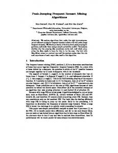
Strongly Correlated Data

Response times obtained for the C20D10K and Mushrooms datasets are given numerically in Tab. 8, and graphically in Fig. 2, respectively. In these two datasets, the number of frequent generators is much less than the total number of frequent itemsets. Hence, using pattern counting inference, Zart has to perform much fewer support counts than Apriori. We can observe that in all cases the execution times of Zart and Pascal are almost identical: adding the frequent closed itemset derivation and the identification of their generators to the frequent itemset discovery does not induce serious additional computation time. Apriori is very efficient on sparse datasets, but on strongly correlated data the other two algorithms perform much better.


17

Table 8. Response times of Zart and other statistics min supp (%) Apriori Pascal Zart T20I6D100K 2 1 0.75 0.5 0.25 C20D10K 50 40 30 20 10 Mushrooms 60 50 40 30 20

#F CIs #F Is

#F Gs #F Is

378 1,534 4,710 26,305 149,447

100.00% 100.00% 100.00% 97.66% 96.17%

100.00% 100.00% 100.00% 98.02% 96.32%

456 544 951 2,519 8,777

456 544 967 2,671 9,331

25.01% 25.01% 17.88% 12.45% 9.76%

25.01% 25.01% 18.18% 13.20% 10.38%

19 45 124 425 1,169

21 53 153 544 1,704

37.25% 27.61% 24.55% 16.43% 2.19%

41.18% 32.52% 30.30% 21.03% 3.19%

# FIs # FCIs # FGs

72.67 107.63 134.49 236.10 581.11

71.15 106.24 132.00 228.37 562.47

71.13 378 378 107.69 1,534 1,534 133.00 4,710 4,710 230.17 26,836 26,208 577.69 155,163 149,217

61.18 71.60 123.57 334.87 844.44

16.68 19.10 26.74 53.28 110.78

17.94 1,823 19.22 2,175 26.88 5,319 54.13 20,239 118.09 89,883

3.10 2.04 2.05 6.03 3.13 3.13 13.93 6.00 5.94 46.18 12.79 12.75 554.95 30.30 34.88

51 163 505 2,587 53,337

Comparing Pascal+ and Pascal

6.3

We also compared the efficiency of Pascal+ with Pascal. Pascal+ gives almost equivalent response times to Pascal on both weakly and strongly correlated data, i.e. the filtering of closed itemsets among frequent itemsets is not an expensive step. As Pascal is more efficient than Apriori on strongly correlated data (see Tab. 8), Pascal+ is necessarily more efficient than Apriori-Close. If we need both frequent and frequent closed itemsets then Pascal+ is recommended instead of Apriori-Close.

C20D10K

mushrooms Apriori Pascal Zart

140

Apriori Pascal Zart

50

120 40

80

time (s)

time (s)

100

30

60 20 40 10 20

0

0 50

45

40

35

30 25 minimum support (%)

20

15

10

60

55

50

Fig. 2. Response times graphically

45

40 35 minimum support (%)

30

25

20

18

7


Conclusion and Future Work

In this paper we presented a multifunctional itemset miner algorithm called Zart, which is a refinement of Pascal. With pattern counting inference, using the generators of equivalence classes, it can reduce the number of itemsets counted and the number of database passes. In addition, it can identify frequent closed itemsets among frequent itemsets, and it can associate generators to their closure. We showed that these extra features are required for the generation of minimal nonredundant association rules. Zart can also be specified to another algorithm that we call Pascal+ . Pascal+ finds both frequent and frequent closed itemsets, like Apriori-Close. We compared the performance of Zart with Apriori and Pascal. The results showed that Zart gives almost equivalent response times to Pascal on both weakly and strongly correlated data, though Zart also identifies closed itemsets and their generators. An interesting question is the following: can the idea of Zart be generalized and used for any arbitrary frequent itemset miner algorithm, be it either breadthfirst or depth-first? Could we somehow extend these algorithms in a universal way to produce such results that can be used directly to generate not only all strong association rules, but minimal non-redundant association rules too? We think that the answer is positive, but detailed study of this will be subject of further research.

References 1. Bastide, Y., Taouil, R., Pasquier, N., Stumme, G., Lakhal, L.: Mining minimal non-redundant association rules using frequent closed itemsets. In Lloyd, J.et al.., ed.: Proc. of the Computational Logic (CL’00). Volume 1861 of Lecture Notes in Artificial Intelligence – LNAI., Springer (2000) 972–986 2. Kryszkiewicz, M.: Representative association rules. In: PAKDD ’98: Proceedings of the Second Pacific-Asia Conference on Research and Development in Knowledge Discovery and Data Mining, London, UK, Springer-Verlag (1998) 198–209 3. Guigues, J.L., Duquenne, V.: Familles minimales d’implications informatives résultant d’un tableau de données binaires. Mathématiques et Sciences Humaines 95 (1986) 5–18 4. Luxenburger, M.: Implications partielles dans un contexte. Mathématiques, Informatique et Sciences Humaines 113 (1991) 35–55 5. Pasquier, N., Bastide, Y., Taouil, R., Lakhal, L.: Closed set based discovery of small covers for association rules. In: Proc. 15emes Journees Bases de Donnees Avancees, BDA. (1999) 361–381 6. Kryszkiewicz, M.: Concise representations of association rules. In: Pattern Detection and Discovery. (2002) 92–109 7. Pasquier, N., Bastide, Y., Taouil, R., Lakhal, L.: Efficient mining of association rules using closed itemset lattices. Inf. Syst. 24(1) (1999) 25–46 8. Pasquier, N., Bastide, Y., Taouil, R., Lakhal, L.: Discovering frequent closed itemsets for association rules. Lecture Notes in Computer Science 1540 (1999) 398–416 9. Stumme, G., Taouil, R., Bastide, Y., Pasquier, N., Lakhal, L.: Computing Iceberg Concept Lattices with TITANIC. Data and Knowledge Engineering 42(2) (2002) 189–222


19

10. Zaki, M.J., Hsiao, C.J.: CHARM: An Efficient Algorithm for Closed Itemset Mining. In: SIAM International Conference on Data Mining SDM’02. (2002) 33–43 11. Kryszkiewicz, M.: Concise representation of frequent patterns based on disjunctionfree generators. In: ICDM ’01: Proceedings of the 2001 IEEE International Conference on Data Mining, Washington, DC, USA, IEEE Computer Society (2001) 305–312 12. Bastide, Y., Taouil, R., Pasquier, N., Stumme, G., Lakhal, L.: Mining frequent patterns with counting inference. SIGKDD Explor. Newsl. 2(2) (2000) 66–75 13. Boulicaut, J.F., Bykowski, A., Rigotti, C.: Approximation of frequency queries by means of free-sets. In: Proceedings of PKDD 2000, Lyon, France, Springer Berlin / Heidelberg (2000) 75–85 14. Bykowski, A., Rigotti, C.: A condensed representation to find frequent patterns. In: PODS ’01: Proceedings of the twentieth ACM SIGMOD-SIGACT-SIGART symposium on Principles of database systems, ACM Press (2001) 267–273 15. Kryszkiewicz, M., Gajek, M.: Why to apply generalized disjunction-free generators representation of frequent patterns? In Hacid, M.S., Ra, Z., Zighed, D., Kodratoff, Y., eds.: Proceedings of Foundations of Intelligent Systems: 13th International Symposium, ISMIS 2002, Lyon, France, Springer-Verlag Berlin / Heidelberg (2002) 383–392 16. Calders, T., Goethals, B.: Mining all non-derivable frequent itemsets. In: PKDD ’02: Proceedings of the 6th European Conference on Principles of Data Mining and Knowledge Discovery, London, UK, Springer-Verlag (2002) 74–85 17. Calders, T., Goethals, B.: Depth-first non-derivable itemset mining. In: Proc. SIAM Int. Conf. on Data Mining SDM ’05, Newport Beach (USA). (2005) 18. Harms, S., Deogun, J., Saquer, J., Tadesse, T.: Discovering representative episodal association rules from event sequences using frequent closed episode sets and event constraints. In: ICDM ’01: Proceedings of the 2001 IEEE International Conference on Data Mining, Washington, DC, USA, IEEE Computer Society (2001) 603–606 19. Pasquier, N.: Mining association rules using formal concept analysis. In: Proc. of the 8th International Conf. on Conceptual Structures (ICCS ’00), Shaker-Verlag (2000) 259–264 20. Bastide, Y., Taouil, R., Pasquier, N., Stumme, G., Lakhal, L.: Pascal : un algorithme d’extraction des motifs frquents. Technique et science informatiques 21(1) (2002) 65–95 21. Ganter, B., Wille, R.: Formal concept analysis: mathematical foundations. Springer, Berlin/Heidelberg (1999) 22. Agrawal, R., Mannila, H., Srikant, R., Toivonen, H., Verkamo, A.I.: Fast discovery of association rules. In: Advances in knowledge discovery and data mining. American Association for Artificial Intelligence (1996) 307–328 23. Zaki, M.J.: Scalable Algorithms for Association Mining. IEEE Transactions on Knowledge and Data Engineering 12(3) (2000) 372–390 24. Szathmary, L., Napoli, A.: Coron : A framework for levelwise itemset mining algorithms. In Ganter, B., Godin, R., Mephu Nguifo, E., eds.: Suppl. Proc. of ICFCA ’05, Lens, France. (2005) 110–113