A FRAMEWORK AND DATA SOURCES FOR THE

A FRAMEWORK AND DATA SOURCES FOR THE ASSESSMENT OF HUMAN EXPOSURES TO COPPER: The U.S. Situation

Final Technical Report CCL-TR-2002:CERM-04 Prepared for the International Copper Association (ICA Project TPT0619A/BB-00) by P.G. Georgopoulos, S.W. Wang, V.M. Vyas, P.J. Lioy Center for Exposure and Risk Modeling www.cerm.org Environmental and Occupational Health Sciences Institute (EOHSI) UMDNJ – R.W. Johnson Medical School and Rutgers, The State University of NJ 170 Frelinghuysen Road, Piscataway, NJ 08854

and H.C. Tan, I.G. Georgopoulos, J. Yonone-Lioy Nu Horizon Enterprises, Inc. Cranford, NJ 07016

February 2002

Contents Table of Contents

v

List of Figures

vii

List of Tables

x

Acknowledgments

xi

1 INTRODUCTION 1.1 Objective . . . . . . . . . . . . . . . . . . . . . . . . . . . . . . . . . . . . . . 1.2 Rationale . . . . . . . . . . . . . . . . . . . . . . . . . . . . . . . . . . . . . . 1.3 Approach . . . . . . . . . . . . . . . . . . . . . . . . . . . . . . . . . . . . . .

1 1 1 1

2 BACKGROUND AND SIGNIFICANCE 2.1 The NRC [NRC, 2000] Assessment of Chronic Copper Exposure . . . . . . . . . 2.2 Modeling Exposure to Copper in Drinking Water . . . . . . . . . . . . . . . . .

7 8 9

3 APPROACH 3.1 A Population Based Exposure Modeling (PBEM) Framework for Copper . 3.2 Copper Databases - USA . . . . . . . . . . . . . . . . . . . . . . . . . Multimedia Exposure/Biomarker Studies . . . . . . . . . . . . . . . . . 3.2.1 CDC NHANES II & III . . . . . . . . . . . . . . . . . . . . . . . 3.2.2 USEPA NHEXAS . . . . . . . . . . . . . . . . . . . . . . . . . Environmental Releases . . . . . . . . . . . . . . . . . . . . . . . . . . 3.2.3 USEPA TRI . . . . . . . . . . . . . . . . . . . . . . . . . . . . 3.2.4 ATSDR HazDat . . . . . . . . . . . . . . . . . . . . . . . . . . Outdoor Air Quality Measurements . . . . . . . . . . . . . . . . . . . . 3.2.5 USEPA AIRS . . . . . . . . . . . . . . . . . . . . . . . . . . . . Surface and Ground Water, and Sediments . . . . . . . . . . . . . . . . 3.2.6 USGS WQN . . . . . . . . . . . . . . . . . . . . . . . . . . . . 3.2.7 USGS NAWQA . . . . . . . . . . . . . . . . . . . . . . . . . . . 3.2.8 USEPA STORET . . . . . . . . . . . . . . . . . . . . . . . . . 3.2.9 USEPA EMAP . . . . . . . . . . . . . . . . . . . . . . . . . . . Soils and Sediments . . . . . . . . . . . . . . . . . . . . . . . . . . . . 3.2.10 USGS NGA . . . . . . . . . . . . . . . . . . . . . . . . . . . . . Ecological . . . . . . . . . . . . . . . . . . . . . . . . . . . . . . . . . 3.2.11 NOAA Ocean Resources Conservation and Assessment (ORCA) . Drinking Water . . . . . . . . . . . . . . . . . . . . . . . . . . . . . . . 3.2.12 USEPA SDWIS/FED . . . . . . . . . . . . . . . . . . . . . . . Dietary . . . . . . . . . . . . . . . . . . . . . . . . . . . . . . . . . . . 3.2.13 USDA CSFII . . . . . . . . . . . . . . . . . . . . . . . . . . . .

v

. . . . . . . . . . . . . . . . . . . . . . .

. . . . . . . . . . . . . . . . . . . . . . .

. . . . . . . . . . . . . . . . . . . . . . .

. . . . . . . . . . . . . . . . . . . . . . .

19 19 20 20 20 21 22 22 22 23 23 23 23 24 24 24 25 25 25 25 26 26 27 27

3.3 Regional US Copper Databases: New Jersey Examples 3.3.1 Rutgers NJADN . . . . . . . . . . . . . . . . 3.3.2 USGS NJDW . . . . . . . . . . . . . . . . . . 3.4 Regional/International Copper Databases (that include US Territories) . . . . . . . . . . . . . . 3.4.1 AMAP . . . . . . . . . . . . . . . . . . . . . 3.5 Supporting Databases for Exposure Assessment: Human Activities . . . . . . . . . . . . . . . . . . . . 3.5.1 USEPA CHAD . . . . . . . . . . . . . . . . .

. . . . . . . . . . . . . . . . . . . . . . . . . . . . . . . . . . . . . . . . . .

27 27 27

. . . . . . . . . . . . . . . . . . . . . . . . . . . .

28 28

. . . . . . . . . . . . . . . . . . . . . . . . . . . .

28 28

4 DEMONSTRATION CASE STUDY OF COPPER EXIS-USA

57

5 BIBLIOGRAPHY

73

A COPPER DATABASES - USA

75

B REGIONAL US COPPER DATABASES: NEW JERSEY EXAMPLES

129

C REGIONAL/INTERNATIONAL COPPER DATABASES

135

D SUPPORTING DATABASES FOR EXPOSURE ASSESSMENT

149

E ACRONYMS

155

vi

List of Figures 1 2 3

4

5

6

7 8 9 10 11

12 13 14 15 16 17

A unified multimedia/multiscale framework to support human/ecological exposure assessments for copper . . . . . . . . . . . . . . . . . . . . . . . . . . . . . . . Schematic depiction of the databases, models, and flow of information of the overall structure of Copper EXIS-USA the MENTOR framework . . . . . . . . . An example of data retrieval from the Copper Environmental/Exposure Information System. This example demonstrates the retrieval and mapping of copper point source releases to air for 1995. . . . . . . . . . . . . . . . . . . . . . . . Estimates of US population demographic variation in estimated copper intake from food and supplements. Based on NHANES-III nationwide survey data as reported in [NRC, 2000]. (a) males (b) females. . . . . . . . . . . . . . . . . . Estimates of US population demographic variation in estimated copper intake from food and supplements normalized by body weight. Based on NRC (2000) with data from the NHANES III nationwide survey. (a) males (b) females. . . . Estimated daily tap-water consumption distribution for US (from NRC, 2000). Based on the USDA 1994-1996 Continuing Survey of Food Intake by Individuals (CSFII). . . . . . . . . . . . . . . . . . . . . . . . . . . . . . . . . . . . . . . Information flow for combining activity patterns with copper concentrations in water, in the CHEM model [Lagos et al., 1999]. . . . . . . . . . . . . . . . . . Structure (components and information flows) of the EPANET drinking water distribution model . . . . . . . . . . . . . . . . . . . . . . . . . . . . . . . . . Example EPANET/MIKENET application: estimation of copper distribution in a municipal water network (two suppliers) . . . . . . . . . . . . . . . . . . . . . . Frequency histogram of concentration at network nodes calculated for the example of Figure 9 . . . . . . . . . . . . . . . . . . . . . . . . . . . . . . . . . . . . . Structure of source-to-dose Population Based Exposure Modeling (PBEM) of copper (coupled environmental/microenvironmental/uptake modeling) in the MENTOR framework . . . . . . . . . . . . . . . . . . . . . . . . . . . . . . . . . . Air emissions (lb/year) of copper compounds from point sources, for 1998. Data are from USEPA developed Toxics Releases Inventory (TRI). . . . . . . . . . . . Total surface water discharges (lb/year) of copper compounds from point sources, for 1998. Data are from USEPA developed Toxics Releases Inventory (TRI). . . Total underground injection discharges (lb/year) of copper compounds from point sources, for 1998. Data are from USEPA developed Toxics Releases Inventory (TRI). Total air emissions (lb/year) of copper from point sources, for 1998. Data are from USEPA developed Toxics Releases Inventory (TRI). . . . . . . . . . . . . . Total surface water discharges (lb/year) of copper from point sources, for 1998. Data are from USEPA developed Toxics Releases Inventory . . . . . . . . . . . . Total underground injection discharges (lb/year) of copper from point sources, for 1998. Data are from USEPA developed Toxics Releases Inventory (TRI). . . . .

vii

3 4

5

14

15

16 17 30 31 32

33 34 35 36 37 38 39

18 19

20 21 22 23 24

25 26 27 28 29 30 31

32 33 34 35 36 37 38 39

Maximum exceedances (µg/L) of copper in drinking water by USA counties, from the Safe Drinking Water Information System (SDWIS) . . . . . . . . . . . . . . Maximum exceedances of copper in drinking water normalized by county populations (µg/L), by USA counties, from the Safe Drinking Water Information System (SDWIS) . . . . . . . . . . . . . . . . . . . . . . . . . . . . . . . . . . . . . . Mean values of dissolved copper concentrations (µg/L) in surface waters, from WQN . . . . . . . . . . . . . . . . . . . . . . . . . . . . . . . . . . . . . . . . Maximum values of total copper concentrations (µg/L) in surface waters, from WQN . . . . . . . . . . . . . . . . . . . . . . . . . . . . . . . . . . . . . . . . Dissolved copper concentrations (µg/L) in surface waters, from USGS Water Quality Network (WQN) . . . . . . . . . . . . . . . . . . . . . . . . . . . . . . Total copper concentrations (µg/L), 1992-96, in surface waters, from USGS Water Quality Network (WQN) . . . . . . . . . . . . . . . . . . . . . . . . . . . . . . Histogram and summary statistics of dissolved copper concentrations (µg/L) in surface waters, from WQN database. The data are from 671 stations across the U.S. . . . . . . . . . . . . . . . . . . . . . . . . . . . . . . . . . . . . . . . . Histogram and summary statistics of total copper concentrations (µg/L) in surface waters, from WQN database. The data are from 634 stations across the U.S. . . Total copper concentrations (µg/L) in ground waters, from the USGS National Water Quality Assessment (NAWQA) studies . . . . . . . . . . . . . . . . . . . Histogram and summary statistics of copper measurements in groundwater in the NAWQA database, 1992-96. The data are from 534 stations across the U.S. . . Copper concentrations in soils (µg/kg) from the National Geochemical Atlas . . Copper concentrations in sediments and particulate matter (µg/kg) from the National Geochemical Atlas . . . . . . . . . . . . . . . . . . . . . . . . . . . . . . Hierarchy structure for CSFII database . . . . . . . . . . . . . . . . . . . . . . Map of NJADN monitoring station locations. Of these, the Sandy Hook, Jersey City (Liberty Science Center), New Brunswick, Camden, and Pinelands stations have measured wet and dry deposition of copper. . . . . . . . . . . . . . . . . . Dissolved copper concentrations (µg/L) in public supply wells, 1970-1999 . . . . Dissolved copper concentrations (µg/L) in private wells, 1980-2000 . . . . . . . Dissolved copper concentrations (µg/L) in all classes of wells, 1970-2001 . . . . Map of Region V NHEXAS study, identifying Eaton County, Michigan . . . . . . Copper concentrations (µg/L) in standing water, from the NHEXAS USEPA Region V study. . . . . . . . . . . . . . . . . . . . . . . . . . . . . . . . . . . . . Copper concentrations (µg/L) in flushed water, from the NHEXAS USEPA Region V study . . . . . . . . . . . . . . . . . . . . . . . . . . . . . . . . . . . . . . . Copper concentrations (µg/kg) in food, from the NHEXAS USEPA Region V study Copper concentrations (µg/L) in beverages, from the NHEXAS USEPA Region V study . . . . . . . . . . . . . . . . . . . . . . . . . . . . . . . . . . . . . . . .

viii

40

41 42 43 44 45

46 47 48 49 50 51 52

53 54 55 56 60 61 62 63 64

40

41

42

43

44

45

46

The cumulative copper exposure distributions from inhalation, food intake, and drinking water consumption routes for Eaton County, Michigan (calculated by the MENTOR/SHEDS Population Based Model) . . . . . . . . . . . . . . . . . . . The cumulative copper exposure distributions from inhalation, food intake, and drinking water consumption routes as well as total intake for the 1st age group (0 - 4 years old) of Eaton County, Michigan (calculated by the MENTOR/SHEDS Population Based Model) . . . . . . . . . . . . . . . . . . . . . . . . . . . . . The cumulative copper exposure distributions from inhalation, food intake, and drinking water consumption routes as well as total intake for the 2nd age group (5 - 19 years old) of Eaton County, Michigan (calculated by the MENTOR/SHEDS Population Based Model) . . . . . . . . . . . . . . . . . . . . . . . . . . . . . The cumulative copper exposure distributions from inhalation, food intake, and drinking water consumption routes as well as total intake for the 3rd age group (20 - 34 years old) of Eaton County, Michigan (calculated by the MENTOR/SHEDS Population Based Model) . . . . . . . . . . . . . . . . . . . . . . . . . . . . . The cumulative copper exposure distributions from inhalation, food intake, and drinking water consumption routes as well as total intake for the 4th age group (35 - 54 years old) of Eaton County, Michigan (calculated by the MENTOR/SHEDS Population Based Model) . . . . . . . . . . . . . . . . . . . . . . . . . . . . . The cumulative copper exposure distributions from inhalation, food intake, and drinking water consumption routes as well as total intake for the 5th age group (55 - 64 years old) of Eaton County, Michigan (calculated by the MENTOR/SHEDS Population Based Model) . . . . . . . . . . . . . . . . . . . . . . . . . . . . . The cumulative copper exposure distributions from inhalation, food intake, and drinking water consumption routes as well as total intake for the 6th age group (65 years old and above) of Eaton County, Michigan (calculated by the MENTOR/SHEDS Population Based Model) . . . . . . . . . . . . . . . . . . . . . .

ix

65

66

67

68

69

70

71

List of Tables 1 2 3 4 5

Mean and Percentiles for Usual Intake of Copper (mg) from Food, based on the NHANES III (1988 - 1984) survey. From [IOM, 2001] . . . . . . . . . . . . . . Mean and percentiles for usual intake of copper (mg) from food and supplements, calculated from data of the NHANES III (1988 - 1984) survey [IOM, 2001]. . . Mean and percentiles for usual intake of copper (mg) from food, calculated from data of the CSFII (1994-1996) survey [IOM, 2001]. . . . . . . . . . . . . . . . Releases trends from TRI database, for (a) copper and (b) copper compounds, 1988 to 1999 (units: lbs/yr) . . . . . . . . . . . . . . . . . . . . . . . . . . . . Summary profile of general demographic characteristics from Census for Eaton County, Michigan [USCB, 2001] . . . . . . . . . . . . . . . . . . . . . . . . . .

x

11 12 13 29 59

Acknowledgments Support for this work has been provided by the International Copper Association (Project TPT0619A/BB-00). The methods and tools used for the implementation of the U.S. Copper Exposure Information System have been developed by the U.S. EPA funded Center for Exposure and Risk Modeling (CERM) at EOHSI (EPAR-827033). The authors extend their appreciation to Dr. Scott Baker and Mr. Michael Hennelly of the International Copper Association for their helpful comments and insights; Dr. Eric Vowinkel of the US Geological Survey for providing the New Jersey Wells database; and Ms. Linda Everett and Mr. Christos Efstathiou for the preparation of graphics and typesetting of this document.

xi

INTRODUCTION

1

1

INTRODUCTION

1.1

Objective

The overall objective of the work presented here is the development and testing, through a representative case study, of a new integrated, computer-based framework for assessing multimedia/multipathway/multiroute exposures to copper. Since copper is an essential trace element, with low doses resulting in deficiency (Menke’s Disease), but also a toxicant at high doses, it is very important to be able to develop realistic and accurate population exposure assessments. The framework presented here links state-ofthe-art exposure models and databases with Geographic Information Systems (GIS) tools, to provide a versatile approach that allows addressing a wide range of issues regarding population exposures to copper by taking into account the most relevant data. The current implementation of this framework, Copper EXIS-USA (EXIS: Exposure Information System) focuses on an application to the United States of America and includes linkages to databases available for supporting exposure assessments in the US. The methods presented here should be directly transferable to other countries. However, coordinated efforts are required to identify and provide similar archived information and databases for immediate use. Further, data from ongoing studies need to be provided in a form that can be used to construct relational geo databases for use in exposure characterizations.

1.2

Rationale

The rationale of the framework presented here is reflected in the following hypotheses: 1. Consistent coupling of environmental, microenvironmental, and human receptor activity models can improve assessments of multimedia/multipathway/ multiroute exposures to copper. 2. Use of refined data (i.e. specific to a municipality, county, etc. or a watershed etc.) on media relevant to copper exposures (groundwater, municipal water, surficial soil, food, etc.) substantially alters the estimates of exposure (and associated doses), as compared to those derived by default or typical/average values of relevant parameters.

1.3

Approach

This work employs state-of-the-art computational methods and databases to demonstrate the feasibility of evaluating the relative contributions of different 1. media (e.g. water, soil1 , food, airborne dust), 2. pathways (e.g. drinking water, bathing, diet, hand-to-mouth2 , etc.) and 1 2

Implementation of the soil medium is currently in progress. Implementation of the hand-to-mouth pathway is currently in progress.

HUMAN EXPOSURES TO COPPER

2

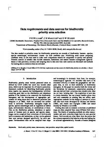
3. routes (e.g. oral, inhalation, dermal3 ) on exposure and target tissue dose. This effort employs a new system (MENTOR, for Modeling Environment for Total Risk Studies) that is being developed through a grant from US EPA. The system includes stateof-the art predictive models of exposure and dose, coupled with tools for retrieving information from up-to-date national, regional, and local databases of environmental, microenvironmental, biological, physiological, demographic, etc. parameters. This open and expandable framework provides a unified and consistent approach for assessing exposure relevant to the multimedia environmental dynamics of copper (see Figure 1). The overall structure of Copper EXIS-USA in the MENTOR framework, depicting schematically the databases, models and flows of information, is presented in Figure 2 (see also [Georgopoulos et al., 2001a, Georgopoulos et al., 2001b]).

3

Implementation of the dermal route is currently in progress.

INTRODUCTION

3

Figure 1: A unified multimedia/multiscale framework to support human/ecological exposure assessments for copper

METEOROLOGICAL DATA: NCDC, AIRS HYDROGEOLOGICAL DATA: USGS GROUND WATER ATLAS DATA FROM EPA EXPOSURE FACTOR HANDBOOK

RELEASES: MULTIMEDIA TRI, HazDat; SITE SPECIFIC

OUTDOOR AIR QUALITY: OBSERVED AIRS, SITE SPECIFIC

DRINKING WATER: SDWIS, NHEXAS; SITE

of Copper EXIS-USA the MENTOR framework

BIOTA: EMAP, ORCA, STORET; SITE SPECIFIC

EXTERNAL MODELS FOR REGIONAL CHARACTERIZATION

"FAST EQUIVALENT" MODELS FOR DISTRIBUTION-BASED POPULATION ASSESSMENTS

HDMR TOOLS FOR SYSTEMATIC MODEL REDUCTION

SUBGRID FATE/ TRANSPORT

STATISTICAL (STRF, BME)

DIAS

MENTOR-BASED OPERATIONS MODELS OF EXPOSURE RELATED ACTIVITIES (FOR INDIVIDUALS & POPULATIONS)

VISUAL FRONT-END FOR CONTINUOUS/DISCRETE EVENT SIMULATION DEFINITION (PLATFORM: STATEFLOW)

MENTOR-BASED PROCESS SOURCE-TO-DOSE MODELS FOR INDIVIDUALS (MICROENVIRONMENTAL AND BIOLOGICAL FATE AND TRANSPORT)

"MULTIMODEL" MENTOR COMPUTATIONAL ENVIRONMENT (PLATFORM: MATLAB 6 WITH FEMLAB 2 TOOLBOX, C++/ JAVA, FORTRAN)

MODULES FOR LOCAL & "NEIGHBORHOOD" SCALE CHARACTERIZION

COUPLED COMPONENTS

HUMAN EXPOSURE: DIETARY - LIFELINE, DEPM, DEEM; INHALATION - PM-SHEDS, HAPEM-4; DRINKING WATER - MM-SHEDS

MULTIMEDIA (SCREENING): MEPAS

OTHER SUPPORTING: EMISSION ALLOCATION - EMS HAP, SMOKE; BIOAVAILABILTY, FOOD WEB, ECOLOGICAL - BLM, CATS, RAMAS-GIS, etc.

DRINKING WATER DISTRIBUTION: EPANET/MIKENET

HYDROGEOLOGIC: SURFACE WATER - SMS, BASINS; WATERSHED - WMS; VADOSE: POREFLOW; GROUNDWATER - GMS, FACT; CHEMISTRY - MINTEQ

ATMOSPHERIC: METEOROLOGY - RAMS, MM5, CALMET; TRANSPORT HYPACT, CALPUFF, AERMOD, ISC; CHEMISTRY/TRANSPORT-CMAQ, REMSAD

GIS FRONT-END FOR SPATIAL PROBLEM DEFINITION AND ANALYSIS (PLATFORM: ARCVIEW, ARCGIS)

MENTOR-BASED EXPOSURE RECEPTOR ATTRIBUTE AND ACTIVITIES INFORMATION SYSTEM (ERAAS)

TOOLS FOR DIAGNOSTIC DATA AND MODEL ANALYSES (PLATFORMS: MATLAB, SAS, SPlus)

CCL's NATIONAL (US) MULTIMEDIA ENVIRONMENTAL INFORMATION SYSTEMS (EIS) FOR SELECTED TOXICS

OBJECT/RELATIONAL AND SPATIAL DATABASE ENGINES: (PLATFORM: ORACLE 9 & ARCGIS/ARCINFO WITH SDE)

SITE SPECIFIC

POPULATION PHYSIOLOGICAL CHARACTERIZATION: NHANES, ICRP

GEOGRAPHIC, LAND USE/COVER, etc.: WESSEX 1ST ST., LANDVIEW IV, USGS

DIETARY: CSFII, NHEXAS; SITE SPECIFIC

HUMAN BIOMARKERS: NHEXAS, NHANES III;

DEMOGRAPHIC SURVEYS: CPS, AHS DIETARY & DRINKING WATER SURVEYS: TDS, CSFII, NHEXAS

SOILS & SEDIMENTS: NGA, NAWQA, EMAP, ORCA, STORET; SITE SPECIFIC

MACRO & MICRO EXPOSURE: CHAD, NHEXAS

SURFACE & GROUND WATER: WQN, EMAP, NAWQA, STORET; SITE SPECIFIC

SPECIFIC

GENERAL/SUPPORTING

CONTAMINANT (AND/OR SITE) SPECIFIC

EXTERNAL DATA SETS (OBSERVATION OR MODEL DERIVED)

4

HUMAN EXPOSURES TO COPPER

Figure 2: Schematic depiction of the databases, models, and flow of information of the overall structure

INTRODUCTION

5

Figure 3: An example of data retrieval from the Copper Environmental/Exposure Information System. This example demonstrates the retrieval and mapping of copper point source releases to air for 1995.

HUMAN EXPOSURES TO COPPER

6

This page is left intentionally blank.

BACKGROUND AND SIGNIFICANCE

2

7

BACKGROUND AND SIGNIFICANCE

As mentioned in the introduction, it is important to be able to assess human population exposures and doses to copper in a realistic and accurate manner, as low intakes of copper can result in deficiency, and high concentrations can result in toxicity. In the general population, there is a range of acceptable intakes that will meet copper requirements and pose no risk of toxicity. According to the Institute of Medicine [IOM, 2001], the primary criterion used to estimate the Recommended Dietary Allowance (RDA) for copper is a combination of indicators, including plasma copper and ceruloplasmin concentrations, erythrocyte superoxide dismutase activity, and platelet copper concentration in controlled human depletion or repletion studies4 . The RDA for adult men and women is 900 µg/day. The median intake of copper from food in the United States is approximately 1.0 to 1.6 mg/day for adult men and women. The Tolerable Upper Intake Level for adults is 10,000 µg/day (10 mg/day), a value based on protection from liver damage as the critical adverse effect 5 . According to the National Research Council [NRC, 2000], copper intake through diet appears to fall within the acceptable range for the average, normal, healthy individual. Furthermore, only a small fraction of an individual’s intake of copper derives from drinking water; and thus, drinking water is not considered to be an important source. However, leaching from copper plumbing could potentially result in some cases in a significant exposure to copper; the potential for copper toxicity is a concern in that case. To address this concern, the National Research Council [NRC, 2000] conducted an analysis intended to provide guidance on the establishment of the maximum contaminant level goal (MCLG). A simplified, nationwide, exposure assessment to copper was performed for that purpose. Furthermore, in order to characterize risks associated with copper exposures, NRC [NRC, 2000] developed certain assumptions/hypotheses regarding the prevalence of sensitive populations and the degree to which copper in drinking water might contribute to copper excess in individuals in those populations. In order to link copper to exposure to risk, NRC [NRC, 2000] considered the hypotheses that a copper sensitivity gene contributes to the hepatic copper toxicity observed in infants 4

Copper functions as a component of a number of metalloenzymes acting as oxidases to achieve the reduction of molecular oxygen. 5 The Institute of Medicine [IOM, 2001] reports, based on data from the 1988 to 1994 Third National Health and Nutrition Examination Survey (Table 2), that the highest median intakes of copper from the diet and supplements for any gender and life stage group were around 1,700 µg/day for males ages 19 through 50 years and 1,600 µg/day for males ages 51 through 70 years and for pregnant and lactating females. The highest reported intake from food and supplements at the ninety-ninth percentile was 4,700 µg/day in lactating females. The next highest reported intake at the ninety-ninth percentile was 4,600 µg/day in pregnant females and males ages 51 through 70 years. In situations where drinking water that contains copper at the present U.S. Environmental Protection Agency (EPA) Maximum Contaminant Level Goal is consumed daily, an additional intake of 2,600 µg copper in adults and 1,000 µg in 1- through 4-year-old children is possible. However, as reported by IPCS [WHO-IPCS, 1998], data from the EPA indicate 98 percent of flushed drinking water samples had copper levels less than 460 µg/L. According to these values, most of the U.S. population receives less than 100 to 900 µg/day of copper from drinking water. Whether total daily intakes of copper will lead to adverse health effects will depend upon the species of copper in the media of concern, its degree of ionization, and its bioavailability.

8

HUMAN EXPOSURES TO COPPER

and young children ingesting increased amounts of copper in milk and water. The current evidence is that manifestations of Tyrolean infantile cirrhosis (TIC), Indian childhood cirrhosis (ICC) and idiopathic copper toxicosis (ICT) involve both heredity and high copper intake [Muller et al., 1996,Muller et al., 1998,Tanner, 1998]. A hypothesis was stated [NRC, 2000] that chronic ingestion of moderately increased amounts of copper produces disease in copper-susceptible genotypes. Furthermore, NRC [NRC, 2000] considered the far more wide ranging hypotheses that heterozygous carriers of the Wilson-disease gene might represent a susceptible group for copper hepatotoxicity, stating evidence that, under current environmental conditions in the United States, the heterozygous carriers accumulate copper and have abnormally high concentrations in the liver and urine. They can be defective in copper handling in the liver as evidenced by Cu incorporation into ceruloplasmin [Brewer et al., 1995]. In addition, unidentified copper sensitivity genes might be responsible for the observed childhood copper toxicity syndromes [Muller et al., 1998, Tanner, 1998]. A heterozygote carrier rate of slightly greater than 1% corresponds to a prevalence rate of 1:40,000 for those homozygous for the Wilson-disease gene. The actual value might be considerably higher (on the order of 2%) if, as expected, the actual prevalence of Wilson disease is underestimated by a factor of approximately 4. Although Wilson heterozygote carriers likely differ in sensitivity, other genetic mutations might also increase copper retention. Thus, according to the NRC hypotheses, at least 1% of the population might be susceptible for increased copper retention on the basis of genetic susceptibility. Provided that increased copper retention confers increased risk of liver toxicity, NRC concluded that groups of this size should be taken into account in establishing the MCLG for chronic exposures.

2.1

The NRC [NRC, 2000] Assessment of Chronic Copper Exposure

The NRC report concluded that comprehensive nationwide survey data for copper in drinking water were not available, and therefore estimates of copper intake via water cannot be estimated accurately. It further stated that clues as to the potential for copper overexposure via tap water come from federal reporting requirements. Under federal law, water systems are required to be sampled for copper in first-draw water (i.e., after water has been motionless for at least 6 hours) at the cold-water tap at locations in the water system vulnerable to copper contamination [USEPA, 1991, USEPA, 1994]. When the 90th percentile of samples taken exceeds 1.3 mg/L, the water purveyor must report that percentile value to the states, which in turn are required to compile and report such values to the U.S. Environmental Protection Agency. In its assessment, NRC [NRC, 2000] used the 90th percentile copper concentrations that water purveyors reported for their systems from 1991 to 1999. The 7,307 values reported correspond to roughly 4,500 individual water systems. With a few exceptions, water systems reporting values greater than 5 mg/L are small, serving 3,300 or fewer people. The majority of those serve nonresidential consumers, such as those at recreational facilities and schools. By law, corrective action might be required for a number of those systems. Nonetheless, the reported 90th percentile concentrations for numerous systems, some of which serve small communities, are notably high, suggesting the potential for copper overexposure.

BACKGROUND AND SIGNIFICANCE

9

From the results of nationwide dietary surveys, copper intake from food was estimated by NRC for different age groups and for the general population (Figures 4 and 5). Dietary survey information was used to evaluate water consumption habits and variations in different age groups. Assuming fixed concentrations of copper, a possible intake of estimate of copper through water can be evaluated. Total copper intake through food and water can then be evaluated. Figure 6 illustrates the calculated total copper intake at different concentrations of copper in water. Based on these calculations, NRC concluded that, at a concentration of 3 mg/L, relatively high copper intake via water could result for some segments of the population.

2.2

Modeling Exposure to Copper in Drinking Water

A detailed model specifically for the calculation of human individual acute and chronic exposure to copper in drinking water, entitled Consumption Habit Exposure Model (CHEM), was developed in Chile [Lagos et al., 1999]. Figure 7 shows the information flow for combining activity patterns with copper concentrations in water, in the CHEM model. The model can estimate daily exposure of individuals, as well as the peak concentration and dose of copper which individuals ingest during a 24-hour period. Evaluation of the model was performed through application, in a limited number of homes, of the Composite Proportional Sampling (CPS) method, used to measure chronic human consumption of contaminants from drinking water. There are three main sources of variability in a population exposure study of copper in drinking water: individual habits variability, chemical variability, and interindividual variability. It was established, mainly in evaluating the model, that the first two sources of variability are crucial for exposure measurement. In some cases these two sources can cancel each other out, whereas, in other cases, they can add to individual exposure estimation error. The CHEM model is not sensitive with respect to an individual’s habits variability because the Water Consumption Habit Survey (WCHS) questionnaire asks for usual behavior. But the CHEM model is very sensitive to chemical variability, i.e. changes in maximum concentration of copper measured on different days. This suggests that in order to minimize estimation error of an individual’s true exposure, measurements of the chemical variables of the model, CMAX , CMIN (the minimum and maximum measured concentrations) and CRAN (a random intermediate concentration), should be made more than once, and preferably three times. It was estimated that for people who stayed at home during the day, CMAX and CMIN weighed an average of 3.8% each, while the rest of copper was ingested at CRAN . For those people who work or study outside the home, the relative weights of CMAX and CMIN was 3.6% and 3.2%, respectively. With respect to acute exposure during the winter period, it was found that 4.5% of the sampled population was exposed to one cup of water or more at the maximum copper concentration available at the tap. The average age of the sample segment, who arises first in the morning and drinks stagnated water, was 41.2 years old. The average age for people who return home in the evening and drink stagnated water, or water with maximum copper concentration, was 63.5 years. In the sample, the probabilities that the different age groups

10

HUMAN EXPOSURES TO COPPER

exposed to one cup or more of water at CMAX during 1 day was 0 for the under 1-year old group: 0.4% for the 1-10-year-old group; 0.8% for the 10-19-year-old group: 3.3% for the 20-64-year-old group, and 1.2% for the over 64-year-old group. The results of acute exposure for the summer were similar to those found for the winter. Finally, in the group of people who get up first, the potentially most exposed group to high concentrations of copper, i.e. segments s.1.1 and s.1.2, were the over 64-year-olds, with 53.4% with respect to the total population of this age group. This group is followed by the 20-64-year-old group, with 41.6%, the 11-19-year-old group with 14.2%, and the 1-10 year-old group with 7.1%, respectively. From the perspective of an essential element, it was estimated that ingestion of copper from drinking water by the population of Santiago was on average 9.0% of the World Health Organization (WHO) recommendation for minimum total ingestion of copper for adults, assuming that 100% of the copper contained in drinking water is absorbed.

BACKGROUND AND SIGNIFICANCE

Sex/Age Categorya 2 to 6mob 7 to 11 mob 1 to 3 yb 4 to 8 y Standard error M 9 to 3y Standard error M 14 to 18 y Standard error M 19 to 30 y Standard error M 31 to 50 y Standard error M 51 to 70 y Standard error M 71+ y Standard error F 9 to 13 y Standard error F 14 to 18 y Standard error F 19 to 30 y Standard error F 31 to 50 y Standard error F 51 to 70 y Standard error F 71+ y Standard error Pregnant Standard error Lactating Standard error All Individuals Standard error All indiv (+P/L) Standard error

N 793 827 3,309 3,448 1,219 909 1,902 2,533 1,942 1,255 1,216 949 1,901 2,939 2,065 1,368 346 99 28,575 29,015

Mean 0.71 0.75 0.74 0.97 0.02 1.24 0.03 1.50 0.05 1.70 0.05 1.67 0.03 1.54 0.03 1.33 0.05 1.08 0.03 1.10 0.05 1.17 0.10 1.18 0.02 1.13 0.02 1.04 0.02 1.28 0.05 1.62 0.11 1.30 0.04 1.30 0.04

11

Percentile 5th 10th 0.30 0.40 0.30 0.40 0.30 0.40 0.70 0.75 0.03 0.03 0.86 0.93 0.03 0.03 0.86 0.97 0.04 0.04 0.96 1.08 0.05 0.05 0.96 1.08 0.02 0.02 0.86 0.97 0.03 0.03 0.75 0.85 0.03 0.03 0.74 0.80 0.03 0.03 0.61 0.69 0.03 0.03 0.67 0.75 0.14 0.13 0.68 0.76 0.03 0.03 0.67 0.75 0.02 0.02 0.63 0.70 0.03 0.02 0.76 0.85 0.06 0.05 0.97 1.09 0.08 0.08 0.72 0.82 0.03 0.03 0.72 0.82 0.03 0.03

25th 0.50 0.50 0.50 0.84 0.03 1.06 0.02 1.17 0.04 1.32 0.05 1.30 0.02 1.19 0.03 1.03 0.03 0.92 0.02 0.84 0.04 0.91 0.12 0.93 0.02 0.90 0.02 0.83 0.02 1.02 0.04 1.31 0.10 0.99 0.04 1.00 0.04

50th 0.70 0.70 0.70 0.96 0.03 1.22 0.03 1.44 0.05 1.63 0.05 1.60 0.03 1.47 0.03 1.27 0.04 1.06 0.02 1.05 0.05 1.12 0.10 1.14 0.03 1.09 0.02 1.01 0.02 1.24 0.04 1.58 0.12 1.24 0.04 1.24 0.04

a

M = male; F = female.

b

Infants and children fed human milk were excluded from all analyses.

75th 0.90 0.90 0.90 1.09 0.03 1.40 0.03 1.76 0.05 2.00 0.06 1.96 0.03 1.81 0.04 1.57 0.05 1.22 0.03 1.30 0.06 1.37 0.09 1.39 0.03 1.32 0.03 1.21 0.02 1.50 0.06 1.89 0.14 1.54 0.05 1.54 0.05

90th 1.00 1.10 1.10 1.21 0.03 1.59 0.04 2.09 0.07 2.39 0.07 2.35 0.05 2.18 0.05 1.88 0.07 1.39 0.04 1.56 0.07 1.64 0.09 1.65 0.04 1.55 0.04 1.43 0.03 1.77 0.09 2.20 0.17 1.86 0.06 1.86 0.06

95th 1.20 1.30 1.30 1.29 0.03 1.70 0.04 2.32 0.08 2.65 0.09 2.61 0.07 2.43 0.07 2.10 0.09 1.49 0.05 1.74 0.09 1.83 0.11 1.83 0.05 1.71 0.05 1.57 0.04 1.95 0.12 2.41 0.19 2.09 0.07 2.09 0.07

99th 1.50 1.70 1.90 1.46 0.05 1.95 0.06 2.80 0.12 3.21 0.13 3.18 0.11 2.97 0.11 2.56 0.14 1.71 0.06 2.13 0.12 2.24 0.17 2.20 0.08 2.05 0.07 1.86 0.06 2.32 0.20 2.82 0.24 2.58 0.10 2.59 0.10

Data are limited to individuals who provided a complete and reliable 24-hour dietary recall on Day 1. Females who had “blank but applicable” pregnancy and lactating status data or who responded “I don’t know” to questions on pregnancy and lactating status were excluded from all analyses. Females who were both pregnant and lactating were included in both the “Pregnant” and “Lactating” categories. The sample sizes for the groups of Pregnant and Lactating females are very small. Estimates of usual intake distributions for those groups are not reliable. The intake distributions for infants 2-6 months, 7-11 months, and 1-3 years of age are unadjusted. Means and percentiles for these groups were computed using SAS PROC UNIVARIATE. For all other groups, data were adjusted using the ISU method. Mean, standard errors, and percentiles were obtained using C-Side. Standard errors were estimated via jackknife replication. Each standard error has 49 degrees of freedom. SOURCE: ENVIRON International Corporation and Iowa State University Department of Statistics, 2000.

Table 1: Mean and Percentiles for Usual Intake of Copper (mg) from Food, based on the NHANES III (1988 - 1984) survey. From [IOM, 2001]

HUMAN EXPOSURES TO COPPER

12

Sex/Age Categorya 2 to 6 mob 7 to 11 mob 1 to 3 yb 4 to 8 y M 9 to 13 y M 14 to 18 y M 19 to 30 y M 31 to 50 y M 51 to 70 y M 71+ y F 9 to 13 y F 14 to 18 y F 19 to 30 y F 31 to 50 y F 51 to 70 y F 71+ y Pregnant Lactating All Individuals All indiv (+P/L)

N 793 827 3,309 3,448 1,219 909 1,900 2,533 1,942 1,255 1,216 949 1,901 2,939 2,065 1,368 346 99 28,575 29,015

Mean 0.71 0.75 0.74 1.05 1.28 1.58 1.85 1.85 1.79 2.20 1.13 1.15 1.32 1.45 1.45 1.52 1.86 2.14 1.49 1.50

Percentile 5th 10th 0.30 0.40 0.30 0.40 0.30 0.40 0.69 0.75 0.87 0.94 0.90 0.99 0.97 1.13 1.03 1.11 0.91 1.00 0.77 0.94 0.74 0.81 0.64 0.73 0.65 0.74 0.75 0.83 0.64 0.81 0.63 0.71 0.86 1.01 0.97 1.12 0.77 0.85 0.77 0.85

25th 0.50 0.50 0.50 0.86 1.06 1.21 1.35 1.34 1.23 1.09 0.92 0.88 0.97 0.97 0.95 0.85 1.14 1.46 1.01 1.01

50th 0.70 0.70 0.70 0.96 1.21 1.47 1.68 1.67 1.56 1.35 1.07 1.07 1.16 1.22 1.14 1.04 1.32 1.92 1.28 1.28

a

M = male; F = female.

b

Infants and children fed human milk were excluded from all analyses.

75th 0.90 0.90 0.90 1.13 1.42 1.77 2.08 2.04 1.96 1.75 1.20 1.30 1.41 1.50 1.52 1.42 2.82 2.58 1.64 1.64

90th 1.00 1.10 1.10 1.25 1.64 2.24 2.88 2.79 3.15 3.02 1.42 1.61 1.98 2.73 3.01 2.98 3.55 3.58 2.36 2.40

95th 1.20 1.30 1.30 1.58 1.92 2.62 3.55 3.54 3.62 3.47 1.65 1.94 3.07 3.22 3.31 3.21 4.01 4.24 3.22 3.22

99th 1.50 1.70 1.90 3.00 2.95 3.77 4.30 4.29 4.56 4.53 3.07 3.27 4.02 4.04 4.08 3.84 4.60 4.70 4.00 4.04

Data are limited to individuals who provided a complete and reliable 24-hour dietary recall on Day 1. Females who had “blank but applicable” pregnancy and lactating status data or who responded “I don’t know” to questions on pregnancy and lactating status were excluded from all analyses. Females who were both pregnant and lactating were included in both the ‘Pregnant” and “Lactating” categories. The sample sizes for the groups of Pregnant and Lactating females are very small. Estimates of usual intake distributions for those groups are not reliable. The intake distributions for infants 2-6 months, 7-11 months, and 1-3 years of age are unadjusted; the total nutrient intake is the sum of the unadjusted food intake and the daily supplement intake. For all other groups, individual total nutrient intakes were obtained as the sum of the adjusted individual usual intake from food alone and the daily supplement intake. The mean and percentiles of the estimated usual intake distributions were computed using SAS PROC UNIVARIATE. SOURCE: ENVIRON Intemational Corporation and Iowa State University Department of Statistics, 2000.

Table 2: Mean and percentiles for usual intake of copper (mg) from food and supplements, calculated from data of the NHANES III (1988 - 1984) survey [IOM, 2001].

BACKGROUND AND SIGNIFICANCE

Sex/Age Categoryb 0 to 6 monthc Standard error 7 to 11 monthc Standard error 1 to 3 yearsc Standard error 4 to 8years Standard error M 9 to 13 years Standard error M 14 to 18 years Standard error M 19 to 30 years Standard error M 31 to 50 years Standard error M 51 to 70 years Standard error M 71+ years Standard error F 9 to 13 years Standard error F 14 to 18 years Standard error F 19 to 30 years Standard error F 31 to 50 years Standard error F 51 to 70 years Standard error F 71+ years Standard error Pregnantd Standard error d Lactating Standard error All Individuals Standard error AlI Indiv (+P/L) Standard error

N 157 112 1791 1650 552 446 854 1684 1606 674 560 436 760 1614 1539 623 71 42 15058 15170

Mean 0.61 0.02 0.77 0.05 0.71 0.01 0.88 0.01 1.17 0.04 1.45 0.05 1.52 0.03 1.50 0.02 1.44 0.03 1.25 0.03 0.99 0.02 1.07 0.05 1.05 0.02 1.06 0.01 1.05 0.02 1.00 0.04 1.17 0.06 1.35 0.11 1.17 0.01 1.17 0.01

Percentile 5th 10th 0.40 0.44 0.02 0.02 0.49 0.55 0.04 0.04 0.41 0.47 0.01 0.01 0.55 0.61 0.01 0.01 0.69 0.78 0.02 0.02 0.81 0.92 0.03 0.03 0.81 0.92 0.03 0.03 0.84 0.95 0.01 0.02 0.78 0.89 0.02 0.02 0.67 0.77 0.02 0.02 0.64 0.71 0.02 0.02 0.62 0.69 0.04 0.05 0.60 0.68 0.02 0.02 0.62 0.70 0.01 0.01 0.63 0.70 0.01 0.01 0.56 0.64 0.02 0.02 0.76 0.83 0.04 0.04 0.84 0.92 0.09 0.09 0.58 0.67 0.01 0.01 0.58 0.67 0.01 0.01

13

25th 0.51 0.02 0.65 0.05 0.56 0.01 0.73 0.01 0.94 0.04 1.12 0.03 1.14 0.06 1.16 0.02 1.08 0.02 0.95 0.04 0.82 0.02 0.82 0.03 0.82 0.02 0.84 0.01 0.83 0.01 0.75 0.02 0.96 0.05 1.08 0.09 0.85 0.01 0.85 0.01

50th 0.60 0.02 0.75 0.04 0.68 0.01 0.86 0.02 1.13 0.03 1.38 0.04 1.44 0.03 1.43 0.02 1.35 0.03 1.18 0.03 0.96 0.02 1.02 0.05 1.01 0.02 1.02 0.01 1.01 0.02 0.95 0.03 1.13 0.05 1.30 0.10 1.10 0.01 1.10 0.01

75th 0.70 0.03 0.86 0.06 0.83 0.01 1.01 0.02 1.35 0.07 1.69 0.06 1.81 0.08 1.77 0.03 1.69 0.04 1.48 0.05 1.13 0.02 1.27 0.06 1.24 0.03 1.24 0.02 1.21 0.02 1.17 0.04 1.33 0.07 1.55 0.13 1.41 0.01 1.41 0.01

90th 0.80 0.03 0.99 0.07 0.98 0.02 1.18 0.02 1.60 0.07 2.05 0.09 2.19 0.05 2.13 0.04 2.08 0.06 1.80 0.07 1.31 0.03 1.49 0.15 1.47 0.05 1.46 0.03 1.44 0.03 1.42 0.09 1.54 0.08 1.83 0.17 1.76 0.02 1.76 0.02

95th 0.88 0.04 1.10 0.11 1.09 0.02 1.29 0.03 1.79 0.07 2.32 0.12 2.47 0.06 2.40 0.05 2.40 0.11 2.03 0.10 1.43 0.04 1.65 0.16 1.63 0.05 1.60 0.03 1.61 0.05 1.62 0.09 1.68 0.10 2.01 0.20 2.01 0.03 2.00 0.03

99th 1.05 0.05 1.38 0.27 1.33 0.04 1.56 0.05 2.24 0.13 2.95 0.19 3.14 0.12 3.05 0.08 3.10 0.17 2.63 0.27 1.72 0.06 2.09 0.18 2.00 0.09 1.91 0.05 1.98 0.08 2.04 0.19 1.97 0.13 2.42 0.29 2.54 0.04 2.54 0.04

a

Data are limited to individuals who provided two 24-hour dietary recalls. Data were adjusted using the ISU method. Mean, standard errors, and percentiles were obtained using C-Side. Standard errors were estimated via jackknife replication. Each standard error has 43 degrees of freedom.

b

M = male; F = female.

c

Breast-feeding infants and children were excluded from all analyses.

d

One female was pregnant and lactating; she was included in both the “Pregnant” and “Lactating” categories. The sample sizes for the groups of Pregnant and Lactating females are very small. Estimates of usual intake distributions for those groups are not reliable. SOURCE: ENVIRON International Corporation and Iowa State University Department of Statistics, 2000.

Table 3: Mean and percentiles for usual intake of copper (mg) from food, calculated from data of the CSFII (1994-1996) survey [IOM, 2001].

14

HUMAN EXPOSURES TO COPPER

Figure 4: Estimates of US population demographic variation in estimated copper intake from food and supplements. Based on NHANES-III nationwide survey data as reported in [NRC, 2000]. (a) males (b) females.

BACKGROUND AND SIGNIFICANCE

15

Figure 5: Estimates of US population demographic variation in estimated copper intake from food and supplements normalized by body weight. Based on NRC (2000) with data from the NHANES III nationwide survey. (a) males (b) females.

16

HUMAN EXPOSURES TO COPPER

Figure 6: Estimated daily tap-water consumption distribution for US (from NRC, 2000). Based on the USDA 1994-1996 Continuing Survey of Food Intake by Individuals (CSFII).

CHEM model [Lagos et al., 1999].

s1.1.1.1 let water run for 15 seconds before drinking

s1.2.1 use water from other taps and drinks from kitchen tap

s3.2 - at work or study place, do not consume water first in the morning

s1.3 - does not get up first, but drinks water from kettle, which contains first draw water

s3.1 - arrive to work or study place first and consume water immediately

s3 - after breakfast, individuals who work or study outside the home, until they return home

s2 - after breakfast, individuals who stay home during the day

s1.2 - get up first and use water in any activity except drinking

s1.2.1.1 - let water run for 30 seconds before drinking

s1.1 - get up first and drink water before using it in any other activity

s1 - from time of waking up until after breakfast

s1.4 - does not get up first and drinks water at random copper concentration

segmented similarly to s1

s4 - just after returning home in the evening

s1.5 - does not consume tap water in the morning

s5 - individuals who return home in the evening, except first fifteen minutes

BACKGROUND AND SIGNIFICANCE 17

Figure 7: Information flow for combining activity patterns with copper concentrations in water, in the

HUMAN EXPOSURES TO COPPER

18

This page is left intentionally blank.

APPROACH

3

19

APPROACH

3.1

A Population Based Exposure Modeling (PBEM) Framework for Copper

A Population Based Exposure Modeling (PBEM) framework has been developed within MENTOR (Modeling Environment for Total Risk Studies) to characterize the multimedia/multipathway exposure to environmental copper. This modeling framework considers currently three exposure routes to estimate population exposure/dose to environmental agent: inhalation, food intake, and drinking water consumption. (The incorporation of the dermal contact route is currently in progress.) This framework consists of the following steps6 : 1. Estimation of the multimedia background levels of copper (air, water, and food) for the area where the population of interest resides. This can be done in general through a combination of environmental model predictions and measurement studies. 2. Estimation of multimedia levels (indoor air, drinking water, and food concentrations) and temporal profiles of copper in various microenvironments such as residences, offices, restaurants, etc. (a) The air concentrations are obtained by microenvironmental mass-balance model simulations using the inputs from step 1. (b) The drinking water concentrations must be obtained from field study measurements. If such data are not available, the drinking water distribution can be modeled (e.g. via the EPANET/MIKENET model) using treatment plant data to obtain the drinking water concentrations at the tap (see Figure 8)7 . An example of an EPANET/MIKENET application is shown in Figures 9 and 10. (c) The food concentrations can be obtained from survey studies such as CSFII and NHEXAS. 3. Selection of a fixed-size sample population in a way that it statistically reproduces essential demographics (age, gender, race, occupation, education) of the population unit used in the assessment (e.g., a sample of 500 people is typically used to represent the demographics of a given census tract). 4. Retrieval of the matching activity diary record from USEPA’s Consolidated Human Activity Database (CHAD) for each individual of the sample population, based on the individual’s demographic characteristics. 6

These steps mention specifically US databases as the sources of input information for the assessment; however, the approach is universal and in principle could be applied to any location in the world where similar information is available or can be collected. 7 The issue of copper leaching from the distribution network is one of special concern [Schock et al., 1995, Schock et al., 2000]

HUMAN EXPOSURES TO COPPER

20

5. Calculation of inhalation and oral intake rates for the members of the sample population, reflecting/combining the physiological attributes of the study subjects and the activities pursued during the individual exposure events. The inhalation rate is calculated based on the person’s age, gender, and the METS (metabolic equivalent of work) value associated with the activity pursued. The oral intake rates are obtained by extracting the survey records (such as CSFII, TDS, NHEXAS, NHANES, etc.) based on the person’s demographic characteristics. 6. Combination of inhalation and oral intake rates with the corresponding multimedia concentrations of copper for each activity event to assess exposures. 7. Averaging or aggregating exposure estimates over time-units (e.g. days, months, etc.) to characterize the exposure metric of concern. 8. Development of appropriate estimates of dose corresponding to calculated exposure and intake estimates, in conjunction with physiological and activity estimates. 9. Extrapolation of population sample exposures and doses to the entire populations of interest and quantify, to the extent possible, variability and uncertainty in the various components, assessing their effect on the estimates of exposure and dose. The above processes are depicted schematically in the flowchart of Figure 11. A summary of the US databases available to support exposure assessments for copper is presented next; more detailed descriptions are provided in Appendix A.

3.2

Copper Databases - USA

The summary database descriptions that follow are grouped as multimedia exposure/biomarker studies, environmental releases, ambient air, surface groundwater and sediment, soils and sediments, ecological, drinking water, and dietary. Multimedia Exposure/Biomarker Studies 3.2.1

CDC NHANES II & III

The National Health and Nutrition Examination Survey (NHANES) is a series of national examination studies conducted in the United States beginning in 1960. The survey is designed to obtain nationally representative information on the health and nutritional status of the population of the United States through interviews and direct physical examinations. The NHANES II series of the studies, was performed from 1976-1979 and includes similar information regarding copper content in an individual’s diet. While the survey results are not reported to the same resolution as NHANES III, the information found in NHANES II can be grouped into similar categories and coded in the same manner as NHANES III. Thus, an overall intake of copper through food can be determined. Due to a difference in the survey setup, information on copper through dietary supplements cannot be obtained. However,

APPROACH

21

NHANES II does provide a serum copper level which was included in anemia-related blood tests [CDC, 2002]. The NHANES III survey was conducted on a nationwide probability sample of approximately 33,994 persons aged 2 months and older. The 30 topics investigated in the NHANES III include: high blood pressure, high blood cholesterol, obesity, passive smoking, lung disease, osteoporosis, HIV, hepatitis, helicobacter pylori, immunization status, diabetes, allergies, growth and development, blood lead, anemia, food sufficiency, dietary intake-including fats, antioxidants, and nutritional blood measures. Study participants were grouped by age, race, gender and family size. Data are available for 81 counties from four U.S. census regions (South, Southwest, Northeast and West). Copper consumption in milligrams (mg) for each individual in the survey is found primarily from 24-hour dietary recall information. The dietary survey includes the combination foods for multi-component food consumption, individual foods, and variable ingredients for the subjects. The food composition is based on the U.S. Department of Agriculture (USDA) Survey Nutrient Database and University of Minnesota’s Nutrition Coordinating Center (NCC). The survey also accounts for any supplementary vitamins and minerals that may affect the amount of consumption. The totals are then compiled to determine an overall intake. 3.2.2

USEPA NHEXAS

The National Human Exposure Assessment Survey (NHEXAS) was developed by the Office of Research and Development (ORD) of the U.S. Environmental Protection Agency (EPA) early in the 1990s to provide critical information about multipathway, multimedia population exposure distribution to chemical classes. Sample collection began mid-1995 and was completed for all of the projects in late 1997. NHEXAS studies were conducted in three different regions of the U.S. by the following research organizations: • Arizona- University of Arizona, Battelle Memorial Institute, and the Illinois Institute of Technology. • Midwest states of Illinois, Indiana, Michigan, Minnesota, Ohio, and Wisconsin- Research Triangle Institute (RTI) and the Environmental and Occupational Health Sciences Institute (EOHSI) jointly sponsored by University of Medicine and Dentistry of New Jersey (UMDNJ) Rutgers, the State University of New Jersey. • Maryland- Harvard University, Emory University, Johns Hopkins University, and Westat, a survey consulting firm. Researchers worked with the participants to measure the level of chemicals in the air they breathed; in foods and beverages they consumed, including drinking water; in the soil and dust around their homes; and in their blood and urine. Environmental copper levels were measured in Midwest States in tap water and drinking water as well as 536 records for copper in food and beverages.

HUMAN EXPOSURES TO COPPER

22

Environmental Releases 3.2.3

USEPA TRI

TRI (Toxics Releases Inventory) is a publicly available database that contains information on specific chemical releases and other waste management activities, reported annually by certain covered industries as well as by federal facilities. This Inventory was established by section 313 of the Emergency Planning and Community Right-to-Know Act of 1986 (EPCRA). Between the years 1988-1996, more than 2,000 facilities reported copper and/or copper compounds releases each year. Air emissions and surface and groundwater releases are reported in aggregated annual totals (lb/year). Monitoring of releases is not mandatory for TRI, and various estimation techniques are used by individual reporting facilities. Hence, variations in releases between facilities may be partly due to differences in environmental release estimation methods [USEPA, 2001a]. Table 4 shows releases trends from the TRI database, for (a) copper and (b) copper compounds for the years 1988 to 1999 (units: lbs/yr). Figure 12 shows the geographical distribution of total air emissions (lb/yr) of copper compounds from point sources, for 1998. Figure 13 shows total surface water discharges (lb/yr) of copper compounds from point sources, for 1998. Figure 14 shows total underground injection discharges (lb/yr) of copper compounds from point sources, for 1998. Figure 15 shows total air emissions (lb/yr) of copper from point sources, for 1998. Figure 16 shows total surface water discharges (lb/yr) of copper from point sources, for 1998. Figure 17 shows total underground injection discharges (lb/yr) of copper from point sources, for 1998.

3.2.4

ATSDR HazDat

HazDat is a publicly available database developed by ATSDR (Agency for Toxic Substances and Disease Registry). It provides access to information on the release of hazardous substances from Superfund sites or emergency events and on the effects of hazardous substances on the health of human populations. A variety of data can be retrieved by using the search engine (or queries). In this database, copper along with other heavy metal measurement data can be downloaded, although the sampling period and media vary, depending on the site activities. There are 4,395 records for copper measurements found in 1,289 sites (results of 2/4/02). HazDat reports concentrations and releases measured in various media at superfund sites; such as groundwater, soils and sediments, outdoor air, surface water, etc. Toxicological profiles, site descriptions, and details of onsite activities leading to environmental releases are also available [Fay and Mumtaz, 1996].

APPROACH

23

Outdoor Air Quality Measurements 3.2.5

USEPA AIRS

AIRS (Aerometric Information Retrieval System) is a computer-based repository of information about airborne pollution in the United States and various World Health Organization (WHO) member countries. The system is administered by the U.S. Environmental Protection Agency (EPA), Office of Air Quality Planning and Standards (OAQPS), Information Transfer and Program Integration Division (ITPID). AIRS contains the air quality information that OAQPS and state agencies need to carry out their respective programs for improving and maintaining air quality. AIRS provides standard information requirements and information handling procedures, which enables OAQPS to compare and to use data from different states. Data are collected through local, state and national monitoring networks, and reported by state level environmental agencies to EPA. EPA is in charge of the maintenence of records. For PM10 , 24 hour aggregated samples were collected once every six days. New stations are coming online since 1999 for hourly fine PM measurements. Copper content information is provided for the years 1982-2000 for the United States, Mexico, Puerto Rico and the Virgin Islands. COPPER TSP; COPPER PM10; COPPER Course Particulate Matter; COPPER Fine Particulate Matter; COPPER PM10 LC; COPPER PM2.5 LC; COPPER - 63; COPPER (1) CYANIDE; COPPER (SP); COPPER (PRECIP) and COPPER COMPOUNDS are listed [USEPA, 2001b]. Surface and Ground Water, and Sediments 3.2.6

USGS WQN

The U.S. Geological Survey (USGS) has, since 1972, systematically monitored streams and rivers in watersheds throughout the United States for two national stream water-quality networks, the Hydrologic Benchmark Network (HBN) and the National Stream Quality Accounting Network (NASQAN), to provide national and regional descriptions of stream water-quality conditions and trends. The Water Quality Network (WQN) database contains water-quality and streamflow data collected for 679 NASQAN and HBN stations in the United States. The water-quality data include a set of 63 physical, chemical and biological properties analyzed during 60,000 stream visits using relatively consistent sampling and analytical methods. The database also includes information about water-quality and streamflow station attributes e.g. drainage area, latitude, longitude, etc. Data from the networks have been used to describe geographic variations in water-quality concentrations, quantify waterquality trends, estimate rates of chemical flux from watersheds, and investigate relations of water quality to the natural environment and anthropogenic contaminant sources. Separate files are available for trace element parameters and include copper concentrations. The data files include station number, sample collection beginning and ending year, month and day, sample collection time and copper concentrations. Such data files containing Copper data are available for stations in all the water-resources regions (watersheds) [Alexander et al., 1998].

HUMAN EXPOSURES TO COPPER

24

Figure 20 shows mean values of dissolved copper concentrations (µg/L) in surface waters. Figure 21 shows maximum values of total copper concentrations (µg/L) in surface waters. Figure 22 shows dissolved copper concentrations (µg/L) in surface waters. Figure 23 shows total copper concentrations (µg/L) in surface waters. Figure 24 shows a histogram and summary statistics of dissolved copper concentrations (µg/L) in surface waters. Figure 25 shows a histogram and summary statistics of total copper concentrations (µg/L) in surface waters. 3.2.7

USGS NAWQA

The NAWQA (National Water Quality Assessment) program was established by the U.S. Geological Survey (USGS) in 1991. The program systematically collects chemical, biological, and physical water quality data from study units (basins) across the United States and British Columbia. The mission of the U.S.G.S. is to assess the quantity and quality of the earth’s resources within the United States and to provide information for policy-makers. The NAWQA program has an on-line data warehouse that links to a database engine of copper concentration in the United States and British Columbia from 1991 to the present time. The concentration includes copper in ground water, surface water/bed sediment and mixture of surface and ground water with temporal resolution of at least one per measurement location. The recorded data measured copper in bio-tissue, bottom mass or dissolved form. There are currently 11,081 records of copper concentration in the data warehouse. The data are intended to guide the use and protection of the water resources of the United States. Supplemental information on site type and land use is provided to link environmental concentrations to human activities [USGS, 2002]. Figure 26 shows total copper concentrations (µg/L) in ground waters, retrieved from the NAWQA files. Figure 27 shows a histogram and summary statistics of copper measurements in groundwater in the NAWQA database. The data are from 534 stations across the U.S. 3.2.8

USEPA STORET

STORET is an Oracle based database, used for the storage of biological, chemical, and physical data for water. The national database, which is administered by the U.S. Environmental Protection Agency (EPA) covers all states, territories, and jurisdictions of the United States, along with bordering areas of Mexico and Canada. The US Public Health Service developed STORET in 1964 as a collection and reporting system for water quality data. STORET began a modernization effort in early 1992 to take advantage of new technological and information management developments. 3.2.9

USEPA EMAP

The Environmental Monitoring and Assessment Program (EMAP) [Eilers et al., 1987] is a research program to develop the tools necessary to monitor and assess the status and trends of national ecological resources. As a result, EMAP’s data groups conduct environmental

APPROACH

25

stress or indicator research and monitoring on the ecological resources of the United States. In this website you can obtain background and contact information as well as available data and metadata files for each group. There is also a search engine for related bibliographic information. In the case of copper, available data can be found in the Estuarine/Coastal datasets. No copper information could be retrieved from the surface water datasets. Soils and Sediments 3.2.10

USGS NGA

The NGA (National Geochemical Atlas) CD utilizes data that are derived from a subset of the National Uranium Resource Evaluation (NURE) and Hydrogeochemical and Stream Sediment Reconnaissance (HSSR) data that are included in the U.S. Geological Survey OpenFile Report 98-622. Samples consisted of solid samples, including stream, lake, pond, spring, and playa sediments, and soils, collected across the United States in the late 1970’s and early 1980’s. The CD publication is intended to ease the difficulties of usage for geochemical research associated with the previous publications of the same primary data. The NGA CD contains values of copper concentrations in solid samples collected in the continental U.S. It also presents maps showing the spatial distribution for visualization of the copper concentrations. These data were collected during the period of time between 1964 and 1995. There are approximately 204,193 records contained within the CD version. Figure 28 shows copper concentrations in soils, and Figure 29 shows copper concentrations in sediments, retrieved from the NGA database. Ecological 3.2.11

NOAA Ocean Resources Conservation and Assessment (ORCA)

Since 1984, NOAA’s National Status and Trends Program (NS&T) has monitored, on a national scale, spatial and temporal trends of chemical contamination and biological responses to that contamination. Temporal trends are being monitored through the Mussel Watch Program, which analyzes mussels and oysters collected annually at about 200 sites. Spatial trends have been described on a national scale from chemical concentrations measured in surface sediments collected by both the Mussel Watch and Benthic Surveillance Projects from 240 sites distributed throughout the coastal and estuarine United States. The NS&T database contains information about specific regions (Maine, Mexico, Biscayne Bay, Tampa Bay, Los Angeles) a variety of media (Sediment, water, shellfish, fish tissue, fish liver) for specific periods (1984-1996). The geographical information is stored in longitude/latitude coordinates. The downloaded files contain actual measurements of a variety of heavy metals including copper, and other organic compounds. Selected shapefiles (for Arcview) are also included [Lauenstein and Cantillo, 1993].

HUMAN EXPOSURES TO COPPER

26

Drinking Water 3.2.12

USEPA SDWIS/FED

The Safe Drinking Water Information System/Federal Version (SDWIS/FED) is an Environmental Protection Agency (EPA) database storing basic information about the nation’s drinking water supply. This information comes from the states and EPA’s regional offices and is reported for every public water system in the United States. SDWIS/FED stores the information that EPA needs to monitor approximately 175,000 public water systems. Information within this database includes the name of the public water system information about the type of area served by the water system (e.g., households, schools, restaurants, gas stations, or rest areas); number of people served by the water system, operating season (year-round or seasonal); who regulates the water system (typically, states regulate systems within their jurisdictions; EPA currently regulates Tribal systems and systems in Wyoming), when (or if) a water system has violated any national drinking water standard; what (if any) follow-up actions, including enforcement actions, have been taken to make sure the water system returns to compliance following a violation. Access to SDWIS/FED, information is gained through a Freedom of Information Act (FOIA) request or through Envirofacts. The Freedom of Information Act (FOIA) requires federal agencies such as EPA to make data available upon request. Through filing a FOIA request, individuals can access the information contained in SDWIS/FED. These requests are processed through EPA’s Office of Ground Water and Drinking Water. There may be a fee for this service. SDWIS/FED information is available through the Internet or via a Freedon of Information Act request to the EPA. The EPA website, Envirofacts, makes a sub-set of SDWIS/FED information easily available to anyone with access to the Internet. The fact sheet entitled “Information Available From the Safe Drinking Water Information System” available at EPA’s website provides more detailed information on the types of data that are available from SDWIS/FED. SDWIS/FED drinking water information that is not on the Internet is available to the public under the Freedom of Information Act (FOIA). Any individual (including non-U.S. citizens), corporation or association, public interest group, and local, state or foreign government, can request SDWIS/FED information under FOIA. The copper data available are part of US EPA’s effort to estimate occurrence of contaminants in drinking water. The copper concentration data are from sampling Public Water Systems used to supply drinking water. Only records containing values above the Maximum Contaminant Level (MCL) are reported [USEPA, 1998]. Figure 18 shows maximum exceedances (µg/L) of copper in drinking water by USA counties, retrieved from the SDWIS. Figure 19 shows maximum exceedances of copper in drinking water normalized by county populations (µg/L), by USA counties, from the SDWIS.

APPROACH

27

Dietary 3.2.13

USDA CSFII

The US Department of Agriculture, Agricultural Research Service (USDA, ARS) conducted the CSFII (Continuing Survey of Food Intakes by Individuals) survey. A nationally representative sample of individuals of all ages, were asked to provide food intakes on two nonconsecutive days, along with socioeconomic and health-related information. Over 1000 variables were collected on household and individual nutrition intake, food groups, health/disease status, diet, health knowledge, and demographics. Copper content information is provided for each Primary Data Set (PDS) (3088 items) [Jacobs et al., 1998]. Figure 30 illustrates the hierarchy structure of the CSFII database.

3.3

Regional US Copper Databases: New Jersey Examples

In addition to nationwide databases, state and regional organizations maintain databases useful for copper exposure assessments. As an example, two databases available for the state of NJ are described here. 3.3.1

Rutgers NJADN

The New Jersey Atmospheric Deposition Network (NJADN) was established in 1997 by the Department of Environmental Sciences, Rutgers University, with funding from NJ Department for Environmental Protection. Its objective is to gain an understanding of the magnitude of toxic chemical deposition throughout the State, and to assess in-State versus out-of-State sources of air toxic deposition. Target chemicals/species are PCBs, PAHs, a suite of chlorinated pesticides, selected trace metals (including Cu), Hg and nitrogen. Copper concentrations and deposition rates are reported from dry deposition (particulate matter) and wet deposition samples. 24-hour aggregated measurements are made once every 12 days. Initial measurements (97-98) are from two stations in NE New Jersey; currently, some four stations across New Jersey measure copper in dry and wet deposition samples. Data are currently undergoing QA, and are not ready for public release [Eisenreich et al., 1998]. Figure 31 shows a map of NJADN monitoring station locations. Of these, the Sandy Hook, Jersey City (Liberty Science Center), New Brunswick, Camden, and Pinelands stations have measured wet and dry deposition of copper. 3.3.2

USGS NJDW

The New Jersey Drinking Water Database, provided by New Jersey offices of USGS and incorporated into Copper EXIS-USA, looks into the copper in drinking water data for the state of New Jersey. The data file includes station ID, sample collection date and time, pH and copper concentration (µg/L). A total of 2,202 stations were sampled. Some of the stations have more than one record sampled at different dates and times [Vowinkel, 2002]. Figure 32 shows dissolved copper concentrations in public wells; Figure 33 shows dissolved

HUMAN EXPOSURES TO COPPER

28

copper concentrations in private wells; Figure 34 shows dissolved copper concentrations in all classes of wells.

3.4

Regional/International Copper Databases (that include US Territories)

3.4.1

AMAP

The Arctic Monitoring and Assessment Program (AMAP) was established in 1991 to implement components of the Arctic Environmental Protection Strategy (AEPS) which was adopted by the First Arctic Ministerial Conference in 1991. The primary objectives of AMAP are to provide reliable and sufficient information on the status of, and threats to, the Arctic environment, and to provide scientific advice on actions to be taken in order to support countries with Arctic territories in their efforts to take remedial and preventive actions relating to contaminants. These Arctic governments came from eight different countries: Canada, Denmark, Finland, Iceland, Norway, Russia, Sweden, and the United States of America. The AMAP Assessment Report is the first fully referenced report edited and produced by the AMAP. The report contains data on the status of copper as a heavy metal pollutant in the Arctic region. There are 740 records of copper concentrations in various Arctic environmental compartments, such as fresh water sediments, soils, suspended particulate matter in fresh waters, dissolved metal in fresh water, arctic marine sediments and wetlands. These data are an outcome of the first AMAP monitoring program and assessment that were performed between 1991 and 1996. Most of these records are the result of “one-time” measurements by different groups of scientists and researchers from the eight countries with Arctic territories [AMAP, 1998].

3.5

Supporting Databases for Exposure Assessment: Human Activities

3.5.1

USEPA CHAD

The Consolidated Human Activity Database (CHAD), developed for the Environmental Protection Agency’s National Exposure Research Laboratory, consolidates a variety of information from pre-existing human activity studies that were collected at city, state, and national levels. CHAD contains 22,968 person days of activity which span back as far as 1983. All ages and both genders are included in the database, and information regarding every activity undertaken during the day, and lasting for more then 1 minute, is included in sequential order. Participants can be subgrouped by age, weight, race and gender. Supplemental information is provided on housing characteristics, health conditions, presence of smokers, employment information, and prevailing meteorological conditions [USEPA, 2001c].

(units: lbs/yr) Stack Air

532,109 561,726 527,668 743,295 800,625 788,319 972,758 1,090,623 932,856 581,049 806,702 1,204,104

Fugitive Air

1,700,231 347,072 371,242 4,327,401 470,179 413,296 280,882 466,777 359,188 363,790 882,578 320,708

2,232,340 908,798 898,910 5,070,696 1,270,804 1,201,615 1,253,640 1,557,400 1,292,044 944,839 1,689,280 1,524,812

Total Air Emissions

Surface Underground Water Injections Discharges 37,073 62,372 55,401 79,845 41,780 57,513 50,187 41,032 44,997 29,787 56,008 19,944 47,292 23,677 41,819 16,736 59,289 14,011 58,195 22,106 100,975 31,889 116,919 15,646

1999 1998 1997 1996 1995 1994 1993 1992 1991 1990 1989 1988

Year

Stack Air

922,703 955,794 746,837 678,971 1,199,081 2,133,672 3,200,520 2,738,481 1,894,606 1,073,167 844,176 822,028

Fugitive Air

1,289,047 3,170,857 4,743,816 422,822 827,449 3,241,848 4,003,630 3,610,746 2,399,697 868,388 995,481 2,336,964

2,211,750 4,126,651 5,490,653 1,101,793 2,026,530 5,375,520 7,204,150 6,349,227 4,294,303 1,941,555 1,839,657 3,158,992

Total Air Emissions

Surface Underground Water Injections Discharges 361,578 1,521,336 465,178 1,562,046 111,155 237,184 82,195 340,693 93,463 284,852 95,194 214,308 92,426 229,174 81,699 201,431 160,411 224,560 73,213 192,439 141,546 167,941 185,292 165,957

(b) COPPER COMPOUNDS (units: lbs/yr)

1999 1998 1997 1996 1995 1994 1993 1992 1991 1990 1989 1988

Year

(a) COPPER (units: lbs/yr)

Total On-site Releases

16,554,410 281,124,970 2,756,068 8,504,685 3,003,980 2,274,137 2,799,605 14,383,788 16,811,864 12,443,151 11,844,172 12,123,532

Total On-site Releases

1,775,959,051 1,780,053,715 1,285,573,992 1,291,727,867 45,722,127 51,561,119 47,621,144 49,145,825 40,773,223 43,178,068 41,698,059 47,383,081 40,075,738 47,601,488 34,492,794 41,125,151 41,788,248 46,467,522 39,382,784 41,589,991 26,462,036 28,611,180 29,683,607 33,193,848

Releases to Land

14,222,625 280,080,926 1,757,865 3,342,770 1,658,392 996,570 1,474,996 12,767,833 15,446,520 11,418,011 10,022,028 10,466,155

Releases to Land

Total Offsite Releases 16,087,593 16,094,262 10,946,994 8,847,332 10,171,377 12,286,547 14,601,057 10,080,331 8,170,446 47,778,122 10,670,267 14,135,121

Total Offsite Releases 11,442,220 12,310,359 18,478,106 13,622,295 15,001,841 13,971,545 13,348,108 14,572,252 15,350,160 12,988,409 11,528,151 17,233,044

Total On- and Off-site Releases 1,796,141,308 1,307,822,129 62,508,113 57,993,157 53,349,445 59,669,628 62,202,545 51,205,482 54,637,968 89,368,113 39,281,447 47,328,969

Total On- and Off-site Releases 27,996,630 293,435,329 21,234,174 22,126,980 18,005,821 16,245,682 16,147,713 28,956,040 32,162,024 25,431,560 23,372,323 29,356,576

APPROACH 29

Table 4: Releases trends from TRI database, for (a) copper and (b) copper compounds, 1988 to 1999

model

Control Valve: Start & End nodes, diameter, setting, status

Pump: Start & End nodes, pump curve, speed, pattern, initial status, efficiency curve, energy price, price pattern, power

Pipes: Start & End nodes, diameter, length, roughness coeff, status (open/closed/with check valve), bulk reaction coeff, wall reaction coeff

Tank: Bottom elevation, diameter, initial minimum & maximum water levels & water quality, minimum volume, volume curve, mixing model, reaction coeff, source quality

Reservoir: Hydraulic head, initial water quality, head pattern, source quality

Junction: Elevation, water demand, initial water & source quality, demand pattern & categories, emitter coeff

Draw Distribution Network (junctions, reservoir, tank, pipes, pump and control valve)

Junctions: Hydraulic head, pressure, water quality

Select hydraulic, quality, reactions, times or energy option from the browser

Edit Curve (pump, volume, head loss, efficiency), Source Quality, Pattern & Controls

Water age & source tracing

Water quality reactions (bulk reaction & wall reaction)

Control Valves: Flow rate, head loss

Pumps: Flow, head gain

Tank: Hydraulic head, water quality

EPANET

Water quality simulation model (uses lagrangian time-based approach)

Hydraulic simulation model (solves flow continuity and head loss equation by gradient method)

Pipes: Flow Rate, velocity, head loss, Darcy-Weisbach friction factor, avg. reaction rate & water quality

Tabular representation

Map representation

Graphical representation

30

HUMAN EXPOSURES TO COPPER

Figure 8: Structure (components and information flows) of the EPANET drinking water distribution

APPROACH

31

Figure 9: Example EPANET/MIKENET application: estimation of copper distribution in a municipal water network (two suppliers)

32

HUMAN EXPOSURES TO COPPER

Figure 10: Frequency histogram of concentration at network nodes calculated for the example of Figure 9

Obtain random realizations from uncertainty distributions of statistical parameters (that specify variability in model parameters)

START

Select a census tract and generate a hypothetical population comprised of N individuals that match the characteristics of the population in census tract

NO NO

YES

MM SHEDS

Food and drinking water consumption and food composition (CSFII, NHEXAS)

Obtain activity events and associated METs values for each individual based on CHAD-ID

YES

Completed all uncertainty iterations ?

Estimate food and drinking water concentration

YES

Calculate food and drinking water consumption

Calculate fraction of drinking water source from standing water from each individual

Calculate microenvironmental air concentrations in each activity location of the activity event sequence using the exposure model parameters

END

Food and drinking water concentrations

Calculate inhalation rates for each activity event of an individual based on age, gender and METs values

On-line data importing module

CHAD database (consolidated human activities)

Calculate dose for each activity event of an individual based on concentration intake rate and time duration of each activity event

Obtain the matching diary record for each individual based on the characteristics of the individual

Obtained dose for all census tracts in area of interest?

Generate random realizations of exposure model parameters for an individual in the generated population from variability distributions (specified by uncertain statistical parameters)

Outdoor air concentrations

Obtained dose estimate for all N individuals in population ?

NO

Obtain estimates of 1-hr averaged outdoor concentrations in census tract

STRF or BME interpolation

Census tract demographic data

APPROACH 33

.

Figure 11: Structure of source-to-dose Population Based Exposure Modeling (PBEM) of copper

(coupled environmental/microenvironmental/uptake modeling) in the MENTOR framework

USEPA developed Toxics Releases Inventory (TRI).

!

!!

!!

!

!

!

!

!

!!

!!! !!! !!! ! !

! !

!

!

!

!

!

!

! ! !

!

! !

!

!

!

!! ! !!

!

!

!

!

!! ! ! ! ! ! ! !!

!

!!

!

!

!

1 - 20

21 - 250

251 - 580

581 - 2588213

!

!

!

!

TOTAL_AIR_EMISSIONS

!

!

!

!

Cu Compounds - TRI98 [lb/yr]

! !

!

! !! !

!

!

! !!

!!

!

!

!

!

!

!

! !

!

!

!

!! !! !

!

!

!

!

!

!

!

!

!

!

!

!

!

!

!!!!

! !

!

! ! ! !! ! !

!

!!

!

! !!

!

!! !!!

! !

! !! ! !

!

! !!

! ! !!!! !!!!!

! !!!

! !!

!

!

!!

150 300

!

! !!

!

!

!

!

!!!

!

!

600

! ! !

!

!

900

­ 1,200 Kilometers Projection: USA Contiguous Albers Equal Area Conic

0

!

!

!

! ! ! !! ! ! !! !!! !! ! !! ! ! ! ! !! ! ! ! !! ! ! !!! ! ! ! ! ! ! ! ! ! ! ! !!!! !!!! ! ! ! !! ! ! ! !! !! ! ! ! !!! !

!

! !! !! ! ! ! ! !!!!!! ! ! !! ! ! ! ! !!! ! !!! !!!! ! ! ! !!!!!!!! !! !! ! ! !!!!!!!!!!! ! !! !! !! ! ! ! !! !!!!!!! ! ! ! ! ! ! ! !!! ! ! ! !!! ! !! !!!! ! !!! ! ! ! ! ! ! ! ! !!!!! ! ! ! ! ! !! ! !! ! ! ! ! ! ! ! ! ! ! !! ! !! ! ! ! !!! ! !! ! ! ! ! ! ! ! ! ! !!!!!! ! ! ! ! ! ! !!! ! ! !! !!! ! !! ! !! !! ! ! !! !!!! ! ! ! ! !! ! ! !!! !! ! ! ! ! ! !!! !!!! ! ! ! ! !! !!! ! ! ! ! ! ! ! ! ! ! ! !! ! ! ! ! ! ! ! ! ! ! ! ! !! !! ! !!! ! ! ! !! !! ! ! ! ! ! ! ! ! ! ! ! ! ! ! ! !! ! ! ! ! ! ! ! ! ! !!!! !!! !!!! ! ! ! !!! ! ! !! !! ! ! ! ! ! ! ! ! ! ! !

!

!

34

HUMAN EXPOSURES TO COPPER

Figure 12: Air emissions (lb/year) of copper compounds from point sources, for 1998. Data are from

Data are from USEPA developed Toxics Releases Inventory (TRI).

! ! !!

!

!

!

!! !!

!

! !

!

!!

!

!

!

!

!

!

!

!

!

!

!

!

1-5

6 - 108

109 - 460

461 - 62000

!

!

!

!

TOTAL_SURFACE_WATER_DISCHARGE

Cu Compounds - TRI98 [lb/yr]

!

!

!! !!

!

!

!

!

!

!

!

!

!

!

!

!

!!

! !

!

!!

!

!

!

!

!

!

!

!!

!

!

!

!

! !

!

!

!

! ! !!!!

!! !

!

!!

! !

!

!!

! !!!

!! ! !! ! !!

!

! ! ! !

! !

!

!

!!

!

! !! !!!!! !!!

!

! !! ! !! !

!

! !

! !

!

!

!

!

!

! !! !

!

!

!

!

!

!

!

!

!

!

!!

! ! !!! !

!

! !

!!

!

600

! ! ! !! ! ! !! ! !! !! !!! ! ! ! ! !! ! ! ! !! ! !!

! !! !!!

150 300

!

!!

!! !

!

!

!

!

!

!

!

!!!

!!

! !! !

!

!

! !!!

! !

! !!

!

900

! !!

! ! !

! !! ! !

!

­

!! ! ! ! ! !!!! ! ! !!

!

1,200 Kilometers Projection: USA Contiguous Albers Equal Area Conic

0

!

! !! !!!! ! !

!! !

!

!! ! ! ! ! !! !! ! !! !! ! !! ! ! ! !!!! ! !

! ! ! ! ! ! ! !

! ! !

! !

! ! !!

!! !! !! !! !!

!

!

APPROACH 35

Figure 13: Total surface water discharges (lb/year) of copper compounds from point sources, for 1998.

for 1998. Data are from USEPA developed Toxics Releases Inventory (TRI).

3 - 177

178 - 360

361 - 8500

8501 - 1100000

!(

!(

!(

!(

TOTAL_UNDERGROUND_INJECTION

Cu Compounds - TRI98 [lb/yr]

!(

!(

!(

!(

!(

!(

!(

!(

150 300

!( (!

600

900

­ 1,200 Kilometers Projection: USA Contiguous Albers Equal Area Conic

0

!(

36

HUMAN EXPOSURES TO COPPER

Figure 14: Total underground injection discharges (lb/year) of copper compounds from point sources,

!

developed Toxics Releases Inventory (TRI).

!

!

!!

!!

!

!!!

! !! !!! !!!!!! !!!!!!!!!!! !! ! ! !

!!!

!

!

!

!

! !

!

!

!

!

!!

!

1 - 10

11 - 185

186 - 384

385 - 103196

!

!

!

!

TOTAL_AIR_EMISSIONS

Cu - TRI98 [lb/yr]

!!

!! !!!

!

!

!!

!

!! !!

! !

!

!

!

!

!

!

!

!

! ! !!

!

! ! ! !!!!!!!!! !!!!!! ! ! !! !

!! !

!

! !

!

!

!

!

!

! ! !! !! ! ! !! !!! !!! !! !

!

!

!

!

!

!

! !

!

! !

!!

!

!

­

! ! ! !!!! ! ! ! ! !! ! ! ! !! ! ! ! ! ! ! ! !!!!! ! ! ! ! !!! ! ! ! ! !!!!!!!!!!! !!!!!! ! !! ! ! ! ! !!

! !!

150 300 600 900 1,200 Kilometers Projection: USA Contiguous Albers Equal Area Conic

0

!

! !!!!! ! ! ! ! !! ! ! !!!!! !!!! !!! ! !! ! ! ! ! !! !! !!!!!! !!! ! ! ! ! ! ! ! ! ! !!!! ! !! !! ! ! !! ! ! !! ! ! !! ! !! ! ! !! ! !!!!! ! !! ! !!! ! !!! !!!! !!!!! ! ! ! ! ! !! !!! ! !! ! ! ! !! !!!!! ! ! !!!!!!!! ! !! !!!!!!!!! ! !!!! ! !! ! !! !!! !!! !!!! !!! !!!!!! ! !!!! ! ! ! ! ! !!!! !! !! ! !! ! ! !! !!!!! ! ! !!!! !! !!!! ! ! !! ! !!!!! !! !! ! ! ! ! ! ! !! ! ! ! ! !!!!!!! ! ! ! ! ! !!!! ! ! ! !! ! ! ! ! ! ! ! ! ! ! ! ! ! ! !! ! ! !!! !! ! ! ! ! ! ! ! ! !! ! !! ! !! ! ! ! ! ! ! !! ! ! ! ! ! ! ! ! ! ! ! !! !! !!!! ! ! ! ! ! ! ! !! ! !!!!! ! !! ! !! ! !!!!!! !!!! !! !! ! ! ! !! ! !!!!! ! ! ! ! !!! ! !! ! ! ! !! ! !! ! !! ! ! ! !!! ! ! ! ! !! ! !! ! ! !!! ! ! ! ! !! ! ! ! ! ! !! ! ! ! !!!!! ! ! ! ! ! !! ! !! !! ! !! ! ! !!! !! !! !!! ! ! ! ! ! ! !! ! ! ! ! ! ! ! !! ! ! ! ! ! !! ! !! !!! !! ! ! ! ! !! !!!!! !! !!! ! ! ! ! !! ! ! ! ! ! ! ! ! ! !! ! ! ! ! ! ! ! ! ! ! !! ! !! !! ! ! ! ! ! ! !! ! ! ! ! ! ! ! ! !!! ! ! ! !! ! !! ! ! ! ! !! ! !! ! ! ! ! !

!

APPROACH 37

Figure 15: Total air emissions (lb/year) of copper from point sources, for 1998. Data are from USEPA

from USEPA developed Toxics Releases Inventory

!

!

! !!! ! !

!

!

! !

!

1-4

5

6 - 53

54 - 2600

!

!

!

!

TOTAL_SURFACE_WATER_DISCHARGE

Cu - TRI98 [lb/yr]

! ! !

! !

!

!!

!

!

!

!

!!

!

!

!

!

! !

!

!

!

! !

!

!

!

!

! !

!

!

!

!

! ! !

!

!

!

!

!

!

!! !

!

! ! !

!

!

!

!

! ! !

!

! !

!

!

! !

!

!

! !

!

!

!

!

!

!

!

!

! ! !! !!

! ! !!

!!

! !

!

! !

! !

!

!

!

!

!

!

!

!

!

150 300

!!

!

!!

!

!

! !

600

!

!

!

!

! !

!

!

!

! ! ! !!!!

!! !!! ! !

!

!

!

!!

900

!

­

! ! ! ! ! !! !! ! ! ! !! ! ! ! !! ! !!! !

!!

1,200 Kilometers Projection: USA Contiguous Albers Equal Area Conic

0

!!

! !! ! !

!

!! ! ! !

! ! ! ! ! ! ! ! !

! ! ! !! !! !! ! !! ! ! !! ! !!! ! !! ! ! ! !!! ! ! ! ! ! ! ! !! ! ! ! ! ! ! ! !! ! !! ! ! ! ! ! ! ! ! ! ! ! ! ! ! ! ! !! ! ! ! !

! !! ! !

! ! ! ! ! !

!

!

38

HUMAN EXPOSURES TO COPPER

Figure 16: Total surface water discharges (lb/year) of copper from point sources, for 1998. Data are

1

2 - 1500

1501 - 54000

!(

!(

!(

TOTAL_UNDERGROUND_INJECTION

Cu - TRI98 [lb/yr]

!(

!(

0

150 300

600

!(

900

1,200 Kilometers Projection: USA Contiguous Albers Equal Area Conic

39

­

APPROACH

Figure 17: Total underground injection discharges (lb/year) of copper from point sources, for 1998. Data are from USEPA developed Toxics Releases Inventory (TRI).

Drinking Water Information System (SDWIS)

>14.40

2.64 - 14.40

2.04 - 2.63

1.68 - 2.03

1.35 - 1.67

Cu Max Exceedance by counties - SDWIS [ug/L]

150 300

600

900

1,200 Kilometers Projection: USA Contiguous Albers Equal Area Conic

0

­

40

HUMAN EXPOSURES TO COPPER

Figure 18: Maximum exceedances (µg/L) of copper in drinking water by USA counties, from the Safe

(µg/L), by USA counties, from the Safe Drinking Water Information System (SDWIS)

> 24.10

3.88 - 24.09

2.49 - 3.87

1.81 - 2.48

1.35 - 1.80

Cu Exceedance Norminalized by County Popu - SDWIS [ug/L]

150 300

600

900

1,200 Kilometers Projection: USA Contiguous Albers Equal Area Conic

0

­

APPROACH 41

Figure 19: Maximum exceedances of copper in drinking water normalized by county populations

42

HUMAN EXPOSURES TO COPPER

Figure 20: Mean values of dissolved copper concentrations (µg/L) in surface waters, from WQN

APPROACH

43

Figure 21: Maximum values of total copper concentrations (µg/L) in surface waters, from WQN

Network (WQN)

!

! ! ! ! ! !!

!

!

! !

! ! ! !

!

! !

!! ! !!

!

!!

!

!

!

!

! !!

!

!

!

1

2

3-4

5-7

8 - 1000

!

!

!

!

!

!

!

!

!

!

! ! !!

!

!

!

!

! !

!

! ! ! ! !

!!

!

! !!

!

!

!

!

!

!

!

!

!

!

! !

!!

!! !! !

!

! !

!

! ! ! !

!! !

!

! ! !

! ! ! ! ! ! !! ! ! ! !

! !

!

!

! !

! ! !!

!

!

! !!

!

! ! !!!!

!

!!

!! ! ! ! !! !! ! !! !

! !

Dissolved Cu - WQN

!

!

!

! !

! ! ! !

!

! ! ! ! ! ! !!

!

!

!

!

!

!

! !

!

!

!

!!

!

!

! ! ! !

!

! ! ! !

!

!

! !

! ! ! !

!

! !

!

!!

! !

!

!

! ! ! ! ! ! !!

!! !

!

!!

!!

!

!

!

!

!

!

! ! !!

!

! !

! !!

!

!! !

!!

!

!

!

! !

! !!

!! ! ! ! !! ! ! !

!! !

! !

!!!! ! ! ! ! ! !! ! ! !! ! ! !! ! ! !!

!

! !

!

!

! ! ! ! !!

­

! ! ! !

! !!

150 300 600 900 1,200 Kilometers Projection: USA Contiguous Albers Equal Area Conic

0

!

!

! ! ! ! ! !!! ! ! ! ! !! ! !! ! ! ! !! ! !! ! ! ! !! ! !! ! ! ! ! ! ! ! !! !! ! ! !! ! !! !

!!! !

! ! ! ! ! ! ! !! ! ! ! ! ! ! !! ! ! ! ! ! ! !! ! ! ! ! ! !! ! !! ! ! ! ! ! !! !! ! ! ! ! ! ! ! ! ! ! ! !! ! ! ! ! ! ! ! ! ! ! ! ! !! ! ! !! ! ! ! ! ! ! !! ! ! ! ! ! ! ! ! ! !! ! ! ! ! ! ! ! !! ! ! ! ! ! ! ! ! ! !! ! ! ! ! ! ! ! ! ! ! ! ! ! !! ! ! !! ! ! ! ! ! ! ! !! ! ! ! !! !! ! !!! !! !! ! ! ! ! ! ! ! !! ! ! ! ! ! ! ! ! ! ! !! ! ! ! ! ! ! ! ! !!!! ! ! ! ! ! ! ! ! ! !! ! ! ! ! ! ! ! ! ! ! ! ! ! !! ! ! !! ! ! !! !!!! !! ! ! !! ! ! ! !! ! ! !! ! ! ! ! ! ! !

!

!

! ! ! !!

!

!!

!

!

44

HUMAN EXPOSURES TO COPPER

Figure 22: Dissolved copper concentrations (µg/L) in surface waters, from USGS Water Quality

Network (WQN)

! ! ! ! !!!

!

! !

! ! ! !

!

! !! !

!

! ! !!

! !

!

1-4

5-6

7 - 11

12 - 20

21 - 420000

!

!

!

!

!

! !!

!

!

!

! !

! !

!! !

!

!

!

!

!

! ! !!

!

!

!

!

!

! !!

!

! !!

!

!

!

!

!

!

!

!

! !

!

! ! ! ! !

!!

!

!!

!! !! !

!

! !

!

!! !

!

! ! !

! ! ! ! ! ! !! ! ! ! !

! !

!

! !!!

!

! ! !!!!

!!

! ! ! ! !! !! ! !! !

! !

Total Cu - WQN

!

!

!

! ! !

! ! !

!

! ! ! ! ! ! !!

!

!

!

!

!

! !

! !

!

!!

!

!

! ! ! !

!

! ! ! !

!

! !

! ! !! ! !

! !

!

!!

!

!

! ! ! ! ! ! !!

!! ! !!

!!

!

!

!

!

!

! ! !

!

! !

! !!

!

!! !

!!

!

!

!

!!

! !!

! ! ! ! ! ! ! !

!

!!! ! ! ! ! ! !! ! ! !! ! !! ! ! !!

155 310

!

! !

!

!

! ! ! ! !!

620

930

­

! ! ! !

! !

1,240 Kilometers Projection: USA Contiguous Albers Equal Area Conic

0

!

!

! ! ! ! ! ! ! ! !! ! ! !! ! !! ! ! ! !! ! !! ! ! ! !! ! !! ! !! !

!!! ! !! !

!! ! ! ! ! ! !! ! ! ! ! ! !! ! ! ! ! ! ! !! ! ! ! ! ! ! !! ! ! ! !! ! ! ! ! ! ! ! !! ! !! ! !! ! ! ! ! ! !!! ! ! ! ! ! !! ! ! ! ! ! !! ! ! ! ! ! ! ! ! !! ! ! ! !! ! ! ! ! ! ! ! ! ! ! ! ! ! ! !! ! ! ! ! ! ! ! !! ! ! ! ! ! ! ! ! ! !! ! ! ! ! ! ! ! ! ! ! ! ! ! ! !!! ! ! ! ! ! ! !! ! ! ! !! ! ! ! ! !! !! ! ! !! ! ! ! ! ! ! ! ! !! !! ! ! ! ! ! ! !! ! ! ! ! ! !! ! ! ! ! ! ! ! !!!! ! ! ! ! ! ! ! !! ! ! ! ! ! ! !! ! !! ! !!!! !! ! ! ! !! ! ! !! ! ! !! ! ! ! ! ! ! !

!

!

! ! ! !!

!

!!

!

!

APPROACH 45

Figure 23: Total copper concentrations (µg/L), 1992-96, in surface waters, from USGS Water Quality

Non zero Data: 35321/55610

US WQN Histogram [Dissolved Copper] Transformation: Log

Data Source: US WQN Data Time Frame: 1962-1995 Attribute: CU

HUMAN EXPOSURES TO COPPER

46

Figure 24: Histogram and summary statistics of dissolved copper concentrations (µg/L) in surface waters, from WQN database. The data are from 671 stations across the U.S.

Non zero Data: 20266/55610

Data Source: US WQN Data Time Frame: 1962- 1995 Attribute: CU

47

WQN Histogram [Total Copper] Transformation: Log

APPROACH

Figure 25: Histogram and summary statistics of total copper concentrations (µg/L) in surface waters, from WQN database. The data are from 634 stations across the U.S.

Quality Assessment (NAWQA) studies

!

!

6 - 17

18 - 27

28 - 43

44 - 620

!

!

!

!

NAWQA Data

! !!!! !!! !!

! !! ! ! !! !

! !! !!!!!! ! ! ! !! !! ! ! ! ! !!!

! ! !! !! ! ! !

!

! ! ! !!!! !! !

!

! ! !!! ! !

! ! !! ! ! ! !

!

! ! !! !

!

!

! !! ! ! ! !

!

!

!!

!

! ! ! !! ! ! ! !!!!! !

! ! !

!

! !

!! ! ! ! !!!!!!!! ! ! !!!!!! !! ! !!

! ! ! ! ! ! !! ! ! ! !!! !! ! ! ! !

! !

! !! !! ! ! ! ! !! ! ! ! ! ! ! !! ! ! ! !! ! ! ! ! ! !

!

!!

!

! ! !

!

!

! !

!! ! !! !

!

! !!

!

! ! !

! ! !

!

!

! !

!

! ! ! ! ! !

! ! ! !!!

! !!!

!

! !! !

!! ! ! !!!!! ! ! !!!!!! !! ! ! !! ! ! ! !! !!! ! ! ! !!! !! ! ! !! ! !! !! ! ! !! !!! ! ! ! ! !!! ! !! ! !! ! ! ! ! ! !! ! ! !! ! ! ! ! ! ! ! ! ! !!!

!

!! !

! !! ! ! !!! !! ! ! ! !! ! ! ! ! !

­ 150 300 600 900 1,200 Kilometers Projection: USA Contiguous Albers Equal Area Conic

0

!! !! ! ! ! ! ! ! !! ! ! ! !!

!! ! !!!!! !! ! !!! ! !!! ! !! ! ! ! ! !! ! !!!!!! ! ! ! ! !! !!! ! ! !! !

!

! ! ! !! ! ! !!!!! !!!!!!! !! !! ! ! !! !! ! ! ! !! ! ! !! !! ! ! ! ! ! ! !!! !!! !! ! !!!!!! ! !!!! !!!! ! !

!

48

HUMAN EXPOSURES TO COPPER

Figure 26: Total copper concentrations (µg/L) in ground waters, from the USGS National Water

Non zero Data: 541

Data Source: US NAWQA Data Time Frame: 1992 1996 Attribute: CU

49

US NAWQA Histogram [Dissolved Copper in Groundwater]

APPROACH

Figure 27: Histogram and summary statistics of copper measurements in groundwater in the NAWQA database, 1992-96. The data are from 534 stations across the U.S.

5 - 30

31 - 41

42 - 65

66 - 43020

!

!

!

!

Cu Concentration - NG_Atlas

!!!

150 300 600 900 1,200 Kilometers Projection: USA Contiguous Albers Equal Area Conic

0

­

!!!!!!!!!! ! !! !!!!!!!!!!! !!!!! !!! ! !!! !!!!! ! ! !!! !! !!!!!! !!!!! ! !! !!!! !!!!!!!!!!!! !! ! !!!! !!!!!!!!!!!!! ! ! ! !!!!! ! !!!!!! !!! !!!!!!! ! !!!!!!!!! ! !! ! !! !!!!! !!!!! !! !!! ! !!!!!! ! !! !!!!!!!! ! !!! !! !!!!!!!!! !!!!! ! !!! ! ! !!!! !!!!!!!!!!!!!!!!! ! !!!!!!! ! ! ! ! !!! ! !! ! ! ! ! !!!!! !! !!!!!!!!!!!!! !! ! !!!!!!! !!! ! !! !!!! ! !! !!!!!!!!!!!!!!!!!!!!!!!!!!!! !!!!!!!!!!!!!!!!!! !!!!!!!!!!!!!!!!!!!!!!!!!!!!!!!!! !! !! ! !!!! ! !!!!!!!!!!! !!!!!!!!!!!! ! !!! ! ! ! ! !!! !!!!!!! !!!!!!!!!!! !! !!! !!!! ! !!!! ! !!!!!!!!!!!! ! ! !!! ! ! ! !! ! !!!!!!!!!!!!! !!!!!!!!!!!!!!!!!!!!! !!!!!!!!!!!!!!!!!!!!!!!!!!!!!! !!!!!!!!!!!!!! !!! !!!!!!!!!!!!!!! !!!! ! !!!!!! !!!!!!!!! !!!!! ! ! !!!!!!!!!!!!!!!! !! !!!!!!!!!!!!!!!!!! ! !!!!!!! ! !!!!!!!!!!!!!!!!!!!!!!!!!! ! ! !!! !! ! ! ! !! !! ! !!!!!!!!!! !!! !!!!!!! !!!!!! !!!!!!!!!!!!!! !!!!!!!!! !!! !!!! ! !!!!!! !!! !! !!!!!! ! ! ! ! ! ! ! ! ! ! !!!!!!!!!! ! ! ! !!!!!!!!!!!! !! !!! !!!!!!!!!!!!!!!!!!!!!! !!!!! !! ! !!!!!! ! ! !! !!!!!! ! !!! !! !!! ! !! !!!!!!!!!!!!!!!!!! !!!!!! !! !! ! !!!!! ! ! ! ! ! ! ! ! ! ! ! ! ! ! !!!!!!!!!! !!!!! !!!!!!!!!!!!!!!!! !!!!!!! !! !!!!!!!! !! ! ! ! ! ! ! !! ! !! !!! !!!!! ! !!! ! !!! !!!!! !!!!!!!!! ! ! ! ! ! ! ! !!!!! !! !!!! ! ! ! ! ! ! ! ! ! ! !! ! !!!!!!!!! !! ! !! !! !!! ! !!!!!!!!!!! !!!! ! !! !!! ! !!!!!!!!!! ! !!! !!!!!!!!!!!!!!!! !!!!!!!!!! !!! !!!!!!! !!!!!!! ! !!!!!!!!!!!! !!!!!! !!!!! !! !!!!!!!!!!!!!!!! ! ! ! ! ! !!! ! ! ! ! ! ! ! ! ! ! ! ! ! ! ! ! ! !!! !!!!!!! !! !!! !!! !!!!! !! ! ! ! !!! !! !!!! ! !! !!!!!! ! !!! !!!!!!!!!!!!!!!!!!!!!!!!! !!!!!!!!!! !!!!! ! !!!!!!!!!!!! !! ! ! !!! ! !!! ! !!!!!!!!!!!!!!!!!!!!!!! ! !!!!!! !!!!!!!!!!!! !! ! ! ! ! ! ! ! ! ! ! ! ! ! ! ! ! ! ! ! !! ! ! !! ! ! ! ! !! !! !! !!!!!!!!!!!!! !! ! !!!! ! ! ! !!!!!!! ! ! !!! !! !!! ! ! ! ! !!! ! !! !! !!!!!!!! !!!!! ! ! !!! ! ! ! ! ! ! !!!! ! ! ! ! !! ! ! ! ! !! !!!!! ! !!!!!!!!! ! !!!!!!!!!!!!!!!!! !!! !! ! !!!!!!!!! ! !!! ! !!! ! !!!!!!! !!!!!!! !! !! ! !! ! ! !! ! !!!! !!!!!!!!!!! !! ! ! !!!!!!!!!! !!!!!!!!! !!!!!!!! ! ! !!!!!!!!! !! !! !!!! ! ! ! ! ! !!!! ! ! !!!!!!!!! !!! !!!!!! !! ! !!! ! !!!!!!!!! !!! !! !! !! ! !!!! !! !!!!! !!!! !!!! !! !!!! ! !!! !!!! !!!!!! !!!!!! !! ! ! !! !!!! !!!!!! ! !! !!! ! !!!!!!!!! ! !!!!!!!!!! !!!!! !!!! ! !!!!!!!!!!!!!! !!!!!!!!!!! !!! !!! !!!!!!! !!! !!!!!!!!!!!!!!!!!!! !!!!!!!!! !! !!!!!!!! ! !!!!!!! ! !! ! !! !! !!!!!!!! !!!!! ! !!!!! ! !!!!!!!!!!!! ! !!! !! !!!! ! ! !!!! !!!! !!!!!!!!!!!!!! !!!!! !!!!!!! ! ! ! ! ! ! ! ! ! ! ! ! ! ! ! ! !! !!!!!!! !! ! ! ! ! ! ! ! !!!!!!!! !!!!!!! !!!!!! ! !!!! !!!!!!!!!!!!!!!! !!! ! ! ! ! ! ! ! ! ! ! !! !!! ! !! ! !!!! !! !! ! !! !! ! !!!!!!! !!!!! ! !!! !!!!!!!! !! !!!!!!!!!! !!!!!!!!!!!! ! !!!!! ! !!!! !!!!!!! !!!!! !!!! !!! !!!!!!!!!! !! ! !!! ! !! ! !! !! !!!!!!!! !!! !!!!! !! !!! !!! ! !! ! !!!! !!!!!!! !!!!!! !!!!!! !! !!!!!!!!!!!!!!!!!! !!! !!!!!!!!!!!!! !!! !!!! ! !!!! ! ! ! !!!! !!! !! ! !!! ! !!!! !! ! ! !!!! !!!!!! !!!!!! ! !!!! !! !! !! !!! !!!! !! !!!!! !!! ! !!!! !! ! ! ! !!!! !!!!!!!!!!! !!!!!!!! !!!!!!! !! !!!!!!!!!!!!!!!!!! ! ! !!!!!!! ! ! !!! !!!! ! !!!! !!!!! !! !! !!!!!!!!! ! !! !!! !! !!!!!! ! ! ! !!!!!!!!!!!!!! ! !!!!! !!!!! ! !!!! !!! ! ! ! ! !!!! !! !!!!!!!!!!! !!!!!!!!!! !! ! ! ! !!!!! ! !!! ! ! ! ! ! ! ! ! ! ! ! ! ! ! ! ! ! ! ! ! ! ! ! ! ! ! ! ! ! ! ! ! ! ! ! ! ! ! ! ! !!! ! !!!! !!!! !!!! ! ! ! ! ! !!! ! !! !!!!! !! !! !!! !!!!!!!! !! !!!!!!!!! !!! !!!!!!! !!!!!! ! !! ! !!!!!!!!!! !!!!!!!!! !! !!!!!!!!!!!!! ! ! !!!!!!! !!!!!!! !!!!!!!!!!! !! !!! ! ! ! ! ! ! ! ! ! ! ! ! ! ! ! ! ! ! ! ! ! ! ! ! ! ! ! ! ! ! ! ! ! ! ! ! ! ! ! ! ! !!! ! ! ! !! !! !! ! !!!!! ! !!!!!!!!!!! !! ! !!! ! !! !!!! ! ! ! ! !!! !! ! !! ! !!!!! ! !!!!!!! ! ! ! ! ! !!!!!!! !! !! ! !! !!! !!!!! ! !! ! !!!!!!! !!!!!!!!! !!!! !!!!!!!! !! !! !!!!! ! !!!!!!!!! !!!! !! ! ! ! ! ! !! !!!! ! ! !! !!! ! !!!!!! !! !!!!!! ! ! !! ! ! !!!!!!!!!!! ! ! ! ! !!! !!!! !! ! ! ! !!!!! !! !! ! !!! !! !!!!!!!! !!!!! !!!! !!!!! ! ! ! !! ! !!! !! !! ! ! !!!! !!!!!! !!!!!!!!!!!! ! ! !!! ! ! !!!!! !!! ! ! ! !!!!!! ! !!!!!!!!!!!!!! ! !!!! !!!!!!!!!!!!! !!!!!!! ! ! !! !! ! ! ! !! ! ! !!!!!!!!!! !! !!!!!! !!!!!!!!! ! !!!!!!! !!!!! !!!!!! ! ! ! !! !! !!!!!!!!!!! !!!!!!!! !! !!!!!! !!! !! !!!!!!!! ! !!! !! !!!!!! ! !!!!!!!! ! !! ! ! ! !!!!!!! !! ! ! !! !!! !!!!!!!! !!!!! !!! !!!!!!!!!!!!!!!!!!!!! !!! !!!!!!!!!!!! !!! !!!!!!!!! ! !!!!!!!!!!!!! !!!!!!!!!!!!!!!!! ! !! ! !! ! !!!!! ! ! ! ! ! ! ! ! ! ! ! ! ! ! ! ! ! ! ! ! !! ! ! ! ! ! ! !!!! ! ! !! !!! ! ! ! ! !!!! ! ! !!!! ! ! !! ! ! !!!! ! !! !!!!!!!! ! !!! !!!!!!!!!!! !!!!!!! !!!! !!! !! !!! !!! ! !!!!!!!!!!!!!!!!!!!!!! !! !!!!!! !!!!! ! !!!!! !!! ! ! !!! ! !!!!!!! ! !! ! ! !!!!!! !!!!! ! ! ! !!!!!!!!!! ! !! !!! ! !!! !!!!!!!!!! !!!! !!!!!! !! !! !!!! !! !! ! ! ! !! ! ! !!! !! !!! !!! !! !!!! !!!!!!!!! ! !!!!!! !!!!! ! ! !!!!!!!!! !!! ! !!!!! !! !! !! ! !!! !!!!! ! !! !! !!!! ! !!!!! !!! ! ! ! ! ! ! ! ! ! ! ! ! ! ! ! ! ! ! ! ! ! ! ! ! ! ! ! ! ! ! ! !!!!! ! !!! ! !! !!! ! !!! !!!! ! !! ! !! !!! !!! ! ! ! ! !!! ! !!! ! ! ! ! !! !! ! !!!!!!!!!!!!! !!!!!!!!!!!!!!! !!!!!! !!!!!!!!! ! ! !! !! !! !! !! !! ! ! ! !! !!!! ! ! !! !!!! ! ! ! !! ! ! ! ! ! ! ! ! ! ! ! ! ! ! !! !! ! ! ! ! ! ! ! !!!!!!!!! ! !!! !!!!! !!!!! !!!! !! !!!!!!!!!!! !!!! ! ! ! !!!!! ! ! ! !!!! !! !! ! !! ! ! ! !!!!! ! ! ! !! ! !!! ! !!!! ! !!!!! !! ! ! ! !!!!!!!!!!!!!!!!!!!!!!!!!!!! !!!! !!! !!!!!!!!!!!!!!! ! !! !!! !!!!! !!! ! ! ! ! ! !! !! !!!!! ! ! ! ! ! !! ! ! ! ! ! ! ! ! ! !! !!! !!! ! ! !! !! !!!!!!!!!! ! !!!!!!!!! ! !!! !! !! !!! ! ! !!!!!! !!!!!! !! !! !!! !!!! ! !! !!!!! !! !!! ! !!!!!!!!!! !!! !! ! ! !!!! !! !!!!!!!!!! !!!!!!!!!!!!! !!!! !!! !!!!!!!!!!!!!!! !!!!!!!!!!!!! !!!!!!!! !!!!!!!!!! !!!!!!!!! !! !!!!! ! !! !!!!!!!!!! ! ! !!! !!!!!!!!! ! !! ! ! ! !!! ! !!!!!!! ! ! !! ! ! ! !!!!! ! !!!!! !! !!! !! !!! !!!!!!!! !! !! !!!!!!!!!!!!!!!! !!!!!!!!!!!!!!!!!!!!!!!!!!!!!!! !! !! !!!!!!!!!!!! ! !! !!! !!!! ! !! !!! !! ! !!!!!!! !!!!!!!!!! !!!!!!!!!! !!!!!!!! !!!!!!!!! ! ! ! !! ! !!!! !!!! !! !! !! !! ! ! !!!!! !!!!!!! !!!!!! !!!!!!!!!!!!!!!!!!! !!!!! !!!!!!!!!!!!!!!!!!! !!!! !!! !!!! !! ! ! ! !!! !!!!!!!!!!!!!!!!! !!! ! ! ! ! !! !!!! !! !!!! ! !!!!!!!!! !!!!!!! !!!!!!! !!! !! !! !! !! ! !!!!!! ! ! !!!! !! !!!!!!! ! !!! !! !!!!! !!!!!! ! ! !!!!! ! !!!!!!!!!!!!!!!!!!! ! !! !!!! !! !!!!!!!!!!!! ! !!!!!!!!!!!!!!!!!! !!! !!!!!!!!! !!!!!! !!!!!!!!!!! !!! ! !!!!! !!! !!!!!!! !!!!!!!!! !! !!!! !! !!! !!!! ! ! ! ! !!! !!! !!!!!! !!!!!!!!!!!!!!!!! !!! !!! !!!!! ! !!!!!!! ! !! !!! !! ! !! !!!!!!!! !!!!!!! !! !!! ! !!!!!!!!! ! ! !! !!!!!!!!!!!!!!!!!!!!!!!!!!!!!!! !! !!!!! !! !!!!!! !! ! !!! ! !! ! !! !!!!! !!!!! ! !!!!!!!!!! !!!!!! !!! !!!!!! !!! !!! ! ! ! ! ! ! ! ! ! ! ! ! ! ! ! ! ! ! ! ! ! ! ! ! ! ! ! ! ! ! ! ! ! ! ! ! ! ! ! ! ! ! ! !! ! !! !!!! !!!!!!!!!!! ! !! !!!! ! !! ! !!! !! ! ! !!! ! ! !! !!!!!!!!!!!!!!!! !! !!!!!!!!!!!!!!! ! ! ! ! !! !!!!!! ! !!!!! ! ! !! !! !! ! !!! !! ! !!!!!! ! !! !!!! ! !!!!!!!!!! !! !!!!!!!!!!!! !!!!!!!! ! ! ! !! !! ! !! !! !!!!!!!!!!!!! !! !!!!!!!!! ! !!!!!! ! !!!!!!! !!!!!!!!!! !!!! ! !!!!!! !!!!!!!!!!!!! ! !! !!! !! ! !!! !! !!!! !! !! !!!!!!!! !!!!!!!!!!!!!!! !!!!!!!!! ! !! !!!!! !!!! ! ! !!!!! !!! !!!!!!!!!!!!! !!!! !! !!!!!!! !! ! !!!!!!! ! !!!!!! !!!! ! !!! !!!! !!! !!! !!! !! ! !! ! !! !!! !!!!!!!!! !! ! !!! ! ! !!!!!! ! ! ! ! ! ! ! ! ! ! ! ! ! ! ! ! ! ! ! ! ! ! ! ! ! ! ! ! ! ! ! ! !! !!! !! !!!! !!!!! ! !!! !! ! !! !!! !! ! !! !!!!!!!!! !! !!! !!! ! !!!!!!! !!!!!!! ! ! !!!!!!! !! ! !! !! !! ! !!!! ! !!!!! !!!! !! !! ! ! ! !!!!!!!!!! !!!!!!!! !! !!!!!! !!! ! !!!!! !!!! !!!! ! !!!!!!!!!!!!!!!!!!!!!!!!!!!!!!!!!! !!!! !!!!!!!!!!!!! !!! !!!! ! ! !! !!! ! !!!!!!!!!!! ! ! !!! ! !!!!! !!!!!!!!!! !! !!!! ! !!!!!!!!!!!! !!!! ! !!! ! ! ! !!! ! !!!!!! ! !! ! ! !!!!! !! ! !!! ! !! !!!! !! !!!!!!!!!!!!!!!! !! !!! !! !!!!! ! !!!!!! !! ! !! ! !! !! !! ! ! !!!!!!!!!! !! ! ! !! ! !!!! !!! !!!! ! !!! ! !!!!!!!!! !!! ! ! !!!!!!!!! !!!!!! ! ! !! !!!!!! !!!!!!!!!!! !!! !!!!!! !!! !! !!!!! !!!!!!! ! !! !!!!!! !!!!!!!!!!!!! !! ! ! ! ! ! ! ! ! ! ! ! !! ! !! !!!! ! ! !!! !! ! !!!!! ! ! !!!!!!!!!! ! !!!!!!!!!!!!!! !!! !!!!!! ! ! ! !!! ! ! ! !! !!! ! !! ! ! ! ! !! ! ! !!!!!!!!!!! !!!! ! !!!! !!!!!! !!!!!! ! !! !!!! !!!!!!!!! !!! !!!!! ! ! ! ! !!!!!!!!!!!!!!!!!!!! ! !!!!!!!!!!!!!!!!!!! !!!! ! !! ! ! !! ! !! !!!!!!!!!!!!!!!!! ! !!!!!!!!! !!! ! ! !!!! ! ! ! !!!!!! ! ! !! !! ! ! ! ! !!!!!!!!!!!!!! !!!!!!!!! !!!!!!!! !! ! ! !! !!!!!!!!! !!!! !! ! !! !!!! !!!! ! ! !! !!! !! !! ! !! !!!!!!! !!! ! ! !! !!!! !! !! !! ! ! !!! !!! !!!! !!!!!!!!!!!!!! !!!!!!!!!! !! ! ! !!! ! ! !!!!!! !!!! ! ! !!!!! ! !!!!!!!!!!!!!!!!!!!!!!!!! ! ! ! ! ! ! ! ! ! ! ! ! ! ! ! ! ! ! ! !! ! !! !! !! !! !!! ! !! !!!!!! ! !!!!!!!!!!!! !! !!!!! ! !! !!! ! !!!!! !! !! !!!! ! !!! !!!!! !! !!!!! !! ! !!! !!!!!! ! !!!!!! !!!!! ! !! !! !!! !! ! !!!!!!!!!!! !! !! !!!!!! !!!!!!!!!!!!!!!!!!!! !!!!!!!!!!!!!!!! ! !!! ! !!!! !! ! !!!!!!!!!!!!! ! !!!! !! ! !! ! !! ! !!!!! !!!! ! ! ! ! ! ! ! ! ! ! ! ! ! ! ! ! ! ! ! ! ! ! ! ! ! ! ! ! ! ! ! ! ! ! ! ! ! ! ! ! !!!!! ! ! ! ! ! ! ! ! ! !! ! ! !! ! !! ! !!!!! ! !! !! ! !!!! !! !!!!!!!!!!! !!!!!!! !! ! !!!!! !!!!! ! !!!! !! !!! !!! !!! !!! ! ! ! ! !!!!!!!! !!!!!!!!! ! !!!!!!!! !!! !!!! ! !! !! !!! !! ! ! ! !!! !!!! !!! !!!!!! ! !!!!! !!! !! ! !!!! ! !!!!!!! !!! !!!!!!!!!!!!! !! !! !!!!! !! !! !!!! !! !!!!!! ! !! !!! !! !! ! !!!!!!!!!!!!! ! !! !!!!! !!!!!! ! ! ! ! !!!!!! !!!!!! !! ! !!!!! !! !! ! !! ! !!! !!!!!!!! ! ! ! ! ! ! !!! !!!!!! ! !!!!!!!!!!!! !!! ! !!! !! ! !!!!! ! !!!!!!!!! ! !!!!! ! !!!!!!!! ! !! ! !! ! ! ! ! ! ! !! ! !!!! !!! ! !! !! !!!!!! !!! !! !!! !! ! ! !! !!!!!! ! ! !! ! !! !! !! ! !!!!! !! ! !!!! !! !! ! !! !!!!!! !!!!!! ! ! !! ! ! ! ! !!! !!! ! ! ! ! ! ! ! ! ! !!!!!!!!! ! !!!! !! ! !! !! !! !!!!! !! !!!!!!! ! ! ! ! ! ! !! !! !! !!! !! !!!!! ! ! !! !!!!!!!!!!! !! !!! ! !! ! !! ! ! ! !!! ! ! !! !! !! !! !!!!!! ! !!!!!! !! ! ! ! ! ! ! ! !! ! !! !!!! !! !!!! ! !!!!! ! !! ! !! ! ! !! !!!!! !!!! !! ! ! !!!!!! !! !!!!!!! ! !! ! ! !! !! !!!!! ! !! !!!! !! ! ! ! ! ! ! ! !! !! ! !!!! !!! !!! ! ! ! ! !!

50

HUMAN EXPOSURES TO COPPER

Figure 28: Copper concentrations in soils (µg/kg) from the National Geochemical Atlas

Geochemical Atlas

95.006 - 96.311

96.312 - 97.639

97.640 - 99.064

99.065 - 100.000

!

!

!

!

Cu Particles - NG_Atlas

!!!

162.5 325 650 975 1,300 Kilometers Projection: USA Contiguous Albers Equal Area Conic

0

­

!!!!!!!!!! ! !! !!!!!!!!!!! !!!!! !!! ! !!! !!!!! ! ! !!! !! !!!!!! !!!!! ! !! !!!! !!!!!!!!!!!! !! ! !!!! !!!!!!!!!!!!! ! ! ! ! !!!!! ! !!!!!! !!! !!!!!!! ! !!!!!!!!! ! !!!!!! ! !! !!!!!! ! ! ! !! !!! ! ! ! ! ! ! ! ! ! !! ! ! ! ! ! ! ! !!! !!!!! ! !!! ! ! !!!!!!!!!!!!!!!!!!!! !! !!!!!! !!!! ! !! !!!!!!!!!!!!!!! !!!!!!! !!!! ! !!!!! !! !!!!!!!!!!!!!!!!!!!!! ! ! ! !! !!!!!!!!!!!!!!!!!!!!!!!!!!!! !!!!!!!!!!!!!!!!!!! !!!!!!!!!!!!!!!!!!!!!!!!!!!!!!!!!! !! !! ! !!!! ! !!!!!!!!!!!!!!!!!!!!!!!! ! !!! !!! ! !!!!!!! !!!!!!!!!!! !! !!!!!!!! !! !!!! ! !!!!!!!!!!!!!!!!!! !!!! ! ! ! ! !!!! !!! ! ! !! ! ! ! ! ! ! ! ! ! ! ! ! ! ! ! ! ! ! ! ! ! ! ! ! ! ! ! ! ! ! ! ! ! ! ! ! ! ! !!!!!! ! !!!!!!!!!! !!!!! !! !!!!!!!!!!!!!!!!!!! ! !!!! !!! !!!!!!!!!!!! !!!!! !! !! !!! !!!!!! ! !!!!!!!!!!!!!!!!!!!!!!!!!!!!!! ! ! !!! !! ! ! ! !! !! ! !!!!!!!!!!! ! !!!!!!!!!!!!!!!! ! !!!!!!! !!!! !!!!!!! !!!!!! !!!!!!!!!!!!!! ! !!! !!!!!!!!!! !!! !!!! ! !!!!!! !!! !! !!!!!! ! ! ! ! ! ! ! ! ! ! ! ! !!! !! !!! ! !!!!!!!!!!!! !! !! !!!!!!!!!!!!!!!!!!!!!!! !!!!! !! !!!!!!!! ! ! ! ! !!! !! ! !!! ! !! !!!!!!!!!!!!!!!!!! ! ! ! !!!!!!!!!! !! !! ! !!!!! ! ! ! ! ! ! !!!!!!!!!!! !!!!! !!!!!!!!!!!!!!!!!!!! !!!!!!! !! !!!!!!!! !!!! ! ! ! ! ! !! ! !!! !!! !!!!!! ! !!! ! !!! !!!!! !!!!!!!!! ! ! ! ! ! ! ! ! ! !! !! !!! ! !!!!!!!!!!! !!!! ! ! !! !!!!!! ! !!!!!!!!!!!! !!!! !!!! !! !!!!!!!!!!!! !!!! !!! ! !!!!!!!!!! !!!!!!!!!!!!! !! !!! ! !!!!! !!!!!!!!!!!!!!!!!!! !!!!!!!!!!!!! ! ! ! ! ! ! ! ! ! ! ! ! ! ! ! ! ! ! ! ! ! ! ! ! ! ! ! ! ! ! ! ! ! !!! !! !! !!! !!!!!!! !!!!!!!!! !! ! !!! ! !!! !!!!!!!!!!!!!!!!!!!!!!! !!! !!! !!!!!!!!!!! !!! !!!! !!!!!!!!!!!!!!!!! !!!!!!!!! !!!!! !! !!! !!! !!!!! !! ! ! ! ! !!! !! !!!! ! !! ! ! ! ! ! ! !! ! ! ! ! ! ! ! ! ! ! ! ! ! ! ! !! !!! !! !!!!!!!!!! !!! !! ! !! ! !!! !!! ! !! !!!!! !!! !! ! !!! ! !!!!!!!! !! ! !!! !!! !!! ! !!!!!!!!!! !!!!!!!!!!!!!!!!!! ! ! !!!!!!!!!!!!! ! !!! ! !! ! ! ! !!! ! !! !!!!! ! ! ! !!!! ! ! ! ! !! ! ! !! ! !! !! !! !!!!!!!!! ! !!! ! !!! !!!! !!! ! !!!!!!!!!! !!!!!!!!! !! !! !! ! !! ! !!!! !!!!!!!!!!! !! ! ! !!!!!!!!!! !!!!!!!!! !!!!!!!! ! ! !!!!!!!!! !! !! !!!! ! ! ! ! ! !!!! ! ! !!!!!!!!! !!! !!!!!! !! ! !!! ! !!!!!!!!! !!! !! !! !! ! !!!!!! !! !!!!! !!!! !!!! !!! !!!! ! !!! !!!! !!!!!! !!!!!! !! ! ! !! !!!! !!!!!! ! !! !!! ! !!!!!!!!! ! !!!!!!!!!! !!!!! !!!! ! ! !!!!!!!!!!! !!!!!!!!!!! !!! !!! !!!!!!! !!! !! !!!!!!!!!!!!!!! !!!!!!!!! !!!!!!!!!!!! ! !!!!!!! ! !! ! !! !!!!!!!!!!! !!!!! ! !!!!! ! !!!!!!!!!!!! ! !!! !! !!!! ! ! ! ! ! !!!! !!!! !!!!!!!!!!!! !!!!! !!!!!!! ! ! ! ! ! ! ! ! ! ! ! ! ! ! ! ! ! ! ! !!!!!!!! !!!!!!! !!!!!! ! !!!! !!!!!!!!!!!!!!!! !!! ! ! ! ! ! ! ! !! !!! !!! !!!! !! !!!!!!!!!!!!!!!!!!!!!!!!!!! !! !!!!! ! !! ! !!!! !! !! ! !! !! ! !!!!!!!! !!!!! ! ! ! !!!!!! !!!!!!! !!!!! !!!! !!! !!!!!!!!!! !! ! !! ! !!! ! !! !! !!!! !! !! ! ! ! !!!!!!!! !!! !!!!! !! !!! !!! ! !! ! ! !!!! !!! !! !! ! !!!!! ! !!!! ! ! !!! !!!!! !!!!!!!! !!!! !!!!! !! !!!!!!!!!!!!!!!!!!!! !! !!!!!!!!!!!! !!! ! !!!! !! ! ! !!!! !!!!!! !!!!!! ! !! !! !! !! !!! !!!!!! !! !!!!!! !!!!! ! ! ! !!!! !!!!!!!!!!! !!!!!!!! !!!!!!! !! !!!!!!!!!!!!!!!!!! ! ! !!!!!! ! !!! !! ! !! ! !!!! !!!! !!!!! !! !! !!!!!!!!!!! ! !! !!! !! !!!!!! ! ! ! !!!!!!!!!!!!! ! ! !! ! ! ! !!!! !! !! !!!!!!!! !!!!!!!!!!!!!! ! ! ! !!!!! !!! !!!! ! ! ! ! ! ! ! ! ! ! ! ! ! ! ! ! ! ! ! ! ! ! ! ! ! ! ! ! ! ! !!!!!!!! ! !!! !! !! !!!!! !!!! ! !! !!!!! !!!! ! !! ! !!!! ! ! !!!! ! !!! !! ! ! ! ! ! ! !!! ! !! !!!!! !! !! !!! ! ! ! !!!!! !!!!!!!!! !!! !!!!!!!!!!!!!!! !! !! !!! !! !!!!!!! !!!!!!! !!!!!!!!!!! !! !!! ! !! !!!!!!! !!!! !! ! !!!!!!!!!!!!! !!!!!!!!!!!!!!!!! !!!! !!!!!!!!! !!!!!!!! !!!! ! ! ! ! ! ! !!!!!!!!!! !!! ! !!!!!!!!!!! !!! ! ! ! ! !! !! ! !!!!! ! ! !! ! !!!!!!!!! ! !!!!!! !!!!!!! ! ! ! !!!! !!!!!!!!!! !!!! !!!!!!!! !! !! !!!!! ! !!!!!!!!! !!!! !! !!!!!! ! ! !! ! !! ! !!!! ! ! ! ! ! ! ! ! ! !! ! ! ! ! ! ! ! !! ! ! ! ! ! ! ! ! ! ! ! ! ! ! ! ! ! ! ! ! !! ! !!! !!! !!!!! !! !! ! !!! !! !!!!!!!!! !!!!!!!!!!! !!!!! ! !!! !! !! ! ! !!!! !!!!!! !!!!!!!!!!!! ! ! ! !! !! ! ! !!! ! ! ! !! !! ! ! ! !!!!!! ! !!!!!!!!!!!!!! ! !!!! !!!!!!!!!!!!! !!!!!!! ! ! !! ! !!!!!!!!!!! !! !!!!!!! ! ! !!!!!!!!!!! ! !!!!! !!!!! !!!!!! !!!! ! !! !!!!!!! !! ! !! ! !! !! !! !!!!!! !!! !! !!!!!!!! ! !!!!! !! !!!!!! ! !!!!!!!! ! !! ! ! ! !!!!!!! !! ! ! !! !!! !!!!!!!! !!!!! !!! !!!!!!!!!!!!!!!!!!!!! !!! !!!!!!!!!!!! !!! !!!!!!!!! ! !!!!!!!!!!!!! !!!!!!!!!!!!!!!!! ! !! ! !! ! ! ! ! ! ! ! ! ! ! ! ! ! ! ! ! ! ! ! ! ! ! ! ! ! !! ! !! ! ! !!!! !! ! !!! !! ! ! ! !!!! ! ! ! !!!!! ! ! !! ! ! !!!! ! !! !!!!!!!! ! !!! !!!!!!!!!!! !!!!!!! !!!! !!! !! !!! !!! ! !!!!!!!!!!!!!!!!!!!!!! !! !!!!!! !!!!! ! !!!!! !!! ! ! !!! ! !!!!!!! ! !! ! ! !!!!!! !!!!! ! ! ! !!!!!!!!!! !! !! !!! ! !!! !!!!!!!!!! !!!! !!!!!! !! !! !! !! !! !! ! ! ! !! ! ! !!! !! !!! !! ! !! !!!! !!!!!!!!! !!! ! !!!!! !! !! !! ! !!! !!!!!! !!!! ! ! !!!!!!!!! !!!!! !! !! ! !!!! ! !!!!! !!! ! ! ! ! ! ! ! ! ! ! ! ! ! ! ! ! ! ! ! ! ! ! ! ! ! ! ! !! !!! !!!! ! !! ! !! !!!!!!!!!!!!!!!!! ! ! !!!! ! !! !!! !!! ! ! ! ! !!! !! ! ! !!!!!!! ! ! ! ! ! !! ! ! !! !! ! ! ! ! ! ! ! ! ! ! ! ! !! !! !! ! ! ! !! !! ! ! !! ! !!! !! !!!! ! ! !!!! ! !!! !!! !!! ! ! ! ! ! ! ! ! ! ! ! ! ! ! ! ! ! ! ! ! ! ! !! !! ! ! ! ! ! !!!!!!!!! ! !!! !!!!! !!!!! !!!! !! !!!!!!!!!!! !!!! ! ! ! !!!!! ! ! ! !!!! !! !! ! !! ! ! ! !!!!! ! ! ! ! !! ! !!! !!!! ! !!!!! !! ! ! ! !!!!!!!!!!!!!!!!!!!!!!!!!!!! !!!! !!! !!!!!!!!!!!!!!!! ! !! !!! !!!!! !!! ! ! ! ! ! !! !! !!!!! ! ! ! ! !! ! ! ! ! ! ! ! ! ! !! !!! !!! ! ! ! ! ! !! !! !!!!!!!!!! !! !!!!!!!!!! ! !!! !! !! !!!!!! !! !! !!! !!!! ! !! !!!!! !! !!! ! !!!!!!!!!! !!! ! !!!! ! !!!!!! !! ! ! !!!!!!!!!! !!!!!!!!! !! !!!!! ! !! !!! ! !!!!!!!!!!!!!!!!!!!!! !!!! !!! !!!!!!!!!!!!!!!!!!!!!!!!!!!!! !!!!!!! !!!!!!!!!! ! ! !!! !!!!!!!!! ! !! ! !!!!!!! !! ! ! ! !!!!! !!! !!!!! ! !!!!! !! !!! !! !!!!!!!! !! !! !!!!!!!!!!!!!!!! !!!!!!!!!!!!!!!!!!!!!!!!!!!!!!! !! !! !!!!!!!!!!!! ! !! !!! !!!! !!!!!!! !!!!!!!!!! !!!!!!!!!! !!!!!!!! !!!!!!!!! ! !! !!! !! ! ! ! ! !! ! !!!! !!!! !! !! !! !! ! ! !!!!! !!!!!!! !!!!!! !!!!!!!!!!!!!!!!!!! !!!!! !!!!!!!!!!!!!!!!!!!! !!!! !!! !!!! !! ! !!! !!!!!!!!!!!!!!!!! !!! ! ! ! ! ! ! !! !!!! !! !!!! ! !!!!!!!!! !!!!!!! !!!!!!! !!! !! !! !! !! ! !!!!!! ! ! !!!! !! ! !!! !! !!!!! !!!!!! ! ! !!!!! ! !!!!!!!!!!!!!!!!!! ! !!!!!!!! !! !!!! !! !!!!!!!!!!!! ! !!!!!!!!!!!!!!!!!! !!! !!!!!!!!! !!!!!! !!!!!!!!!!! !!! ! !!!!! !!! !!!!!!! !!!!!!!!!! !! !!!! !! !!! !!!! ! ! ! ! !!! !!! !!!!!! !!!!!!!!!!!!!!!!! !!! !!! !!!!! ! !!!!!!! ! !! !!! !! ! !! !!!!!!!! !!!!!!! !! !!! !! ! !!!!!!!!! ! ! !! !!!!!!!!!!!!!!!!!!!!!!!!!!!!!!! !! !!!!! !!!!!! !! ! !!! ! !! ! !! !!!!! !!!!! ! !!!!!!!!!! !!!!!! !!! !!!!!! !!! !!! !! ! ! ! ! ! ! ! ! ! ! ! ! ! ! ! ! ! ! ! ! ! ! ! ! ! ! ! ! ! ! ! ! ! ! ! ! ! ! ! ! ! ! ! ! ! ! ! ! !! !! !!!! !!!!!!!!!! ! !! !!!! ! ! ! !!! ! ! ! !!! ! ! !! !!!!!!!!!!!!!! !! !!!!!!!!!!!!!! ! ! ! ! !! !!!!!! ! !!!!! ! ! !! !! !! ! !!! !! ! !!!!!! ! !! !!!! ! !!!!!!!!!! !! !!!!!!!!!!!! !!!!!!!! ! ! ! !! !! ! !! !! !!!!!!!!!!!!! !! !!!!!!!!! ! !!!!!! ! !!!!!!! !!!!!!!!!! !!! !!!!!!!!!!!!!! ! !!!!!! ! !! !!! !! ! !!! !! !!!! !! !! !!!!!!!! !!!!!!!!!!!!!!! !!!!!!!!! ! !! !!!!! !!!! ! ! !!!!! !!! !!!!!!!!!!!!! !!!! !! !!!!!!! !! ! !!!!!!! ! !!!!!! !!!! ! !!! !!!! !!! !!! !!! !! ! !! ! !! !!! !!!!!!!!! !! ! ! ! !!!!! ! ! ! ! ! !!! ! ! ! ! ! ! ! ! ! ! ! ! ! ! ! ! ! ! ! ! ! ! ! ! ! ! ! ! !! !!! !! !!!! !!!!! ! !!! ! ! !! !!! !! ! !! !!!!!!!! !! !!! !!! ! !!!!!!! !!!!!!! ! ! !!!!!!! !! ! !! !! !! ! !!!! ! !!!!! !!!! !! !! ! ! ! !!!!!!!!!! !!!!!!!! !! !!!!!! !!! ! !!!!! !!!! !!!! ! !!!!!!!!!!!!!!!!!!!!!!!!!!!!!!!!!! !!!! !!!!!!!!!!!!! !!! !!!! ! ! !! !!! ! !!!!!!!!!!! ! ! !!! ! !!!!! !!!!!!!!!! !! !!!! ! !!!!!!!!!!!! !!!! ! !!! ! ! ! !!! ! !!!!!! ! !! ! ! !!!!! !! ! !! !!!! !! ! !!! !!!!!!!!!!!!!!!! !! !!! !! !!!!! !!!! ! !!!!!! !! ! !! ! !! !! !! ! ! !!!!!!!!!! !! ! ! !! ! !!!! !!! ! !!! ! !!! !!!!!!!!! ! ! !!!!!!!!! !!!!!! !!!!!! !!!!!!!!!!! !!! !!!!!! !!! !! !!!!! !!!!!!! ! !! !!!!!! !!!!!!!!!!!!! !! ! ! ! !! ! ! ! ! ! ! ! ! ! !! !!!! ! ! ! !! ! !!! !! ! !!!!!!!!!! ! !!!!!!!!!!!!!! !!! !!!!!! ! ! ! ! !!!!! ! !!! ! ! ! !! !!! ! !! ! ! ! ! !! ! ! !!!!!!!!!!! !!!! ! !!!! !!!!!! !!!!!! ! !! !!!! !!!!!!!!! !!! !!!!! ! ! ! ! !!!!!!!!!!!!!!!!!!!! ! !!!!!!!!!!!!!!!!!!! !!!! ! !! ! ! !! ! !! !!!!!!!!!!!!!!!!! ! !!!!!!!!! !!! ! ! !!!! ! ! ! ! !!!!!! ! ! !! !! ! ! ! !!!!!!!!! !!!! !!!!!!!!! !!!!!!!! ! !! ! !! !!!!!!!!! !!!! !! ! ! !! !!!! !!!! ! ! !! !!! !! !! ! !! !!!!!!! !!! ! ! !! !!!! !! !! !! !!!! ! !!! !!! ! !!!!!!!!!!!!!! !!!!!!!!!! !! ! !!! ! ! ! ! !!!!!! !!!! ! ! !!!!! ! !!!!!!!!!!!!!!!!!!!!!!!!! ! ! ! ! ! ! ! ! ! ! ! ! ! ! ! ! ! ! ! ! ! !! ! !! !! !! !! !!! ! !! !!!!!! ! !!!!!!!!!!!! !!!!! !! !! !!!!! ! !! !!!!!!!!!!! !!! !!!!!!!! ! ! ! ! ! ! ! ! ! ! ! ! ! ! ! ! ! ! ! ! ! ! ! ! ! ! ! ! ! ! ! ! ! ! ! ! ! ! ! ! !!!!!!!!! !! !! !!!!!!!!!!!!!!! !!!! ! ! !!!!! !! !!!! ! !! !! ! !!!! ! !!!!! !! !! ! !!! !!!! !!!!!!!!! ! !!!! ! !!!!!!!!!! !!! !! ! !! !!!! !! ! !!!!!! !!!!!!! ! ! !! ! !!!!!!!!! !! ! !! !!!!!!! !! !!!!!! !! !!! ! !!!!!! !!!!!! ! !! !!!!!!!!!!! !! !!!!!!! !! ! !!!!! !!!!! ! !!!!! !! !!! !!! !!! !!! ! !!!!!!!! ! !!!!!!!! !!! ! ! ! !!!!!!!! !!!! !! !! !!! !! ! ! ! !!! !!!! !!! !!!!!! ! !!!!! !!! !! ! !!!! ! !!!!!!! !!! !!!!!!!!!!!!! !! !! !!!!! !! ! !!!! !! !!!!!! ! !! !!! !! !! ! !!!!!!!!!!!!! ! !! !!!!! !!!!!! ! ! ! ! !!!!!! !!!!!! !! ! !!!!! !!! !! ! !! ! !!! !!!!!!!! ! ! ! ! ! ! ! ! !!!!!!!!!!! !!! ! ! ! ! !! !! ! !!!! !!!! ! !!!!!! ! ! !!!!!!!! ! !! ! !! ! ! !! !!!!!! ! !!!!!!! ! !! !!! !!!!!!! ! !!!!!! !!!! !! !!! !! ! ! ! !!!!!! ! ! !! ! !! !! !! ! !!!!! !! ! !!!! !! !! ! !! !!!!!! !!!!!! ! ! !! ! ! ! !!!! !!! !!! ! ! ! ! ! ! ! ! !!! !!!!! ! !!!! !! !! !! ! !! !!!!! !! !!!!!!! ! ! ! ! ! ! !! ! !!! !! !!!!!! !!! ! ! ! ! !!! ! ! ! !! !!!!!!!!!! ! !!! !!! !! !! !! !! !! !! !!!!!! ! !!!!!! !! ! !! ! ! ! !! ! !! !!!! !!!!!!! ! !!!!!!!! ! ! ! !! ! ! ! ! !!! !!!! !! ! ! !!!!!! !!! ! !! ! ! !!!!!! !! !! !!!!! ! !! !!!! !! ! ! !! ! ! ! !! !! ! !!!! !!! !!! ! ! ! ! !!

APPROACH 51

Figure 29: Copper concentrations in sediments and particulate matter (µg/kg) from the National

HUMAN EXPOSURES TO COPPER

52

HIERARCHY STRUCTURE FOR CSFII DATABASE Describe the metadata (metafield) used to link the 9 records within CSFII database RT = Record Type HIERARCHY LEVELS

RT 15: one record per household general household data

I. Household Data

Linked Field

Household ID (HHID)

RT 50: One record per person for completing the Dietary Health Knowledge Survey (DHKS)

RT 25: One sample per person - repeated data subtracted from RT 20's responded sample person

Linked Field

RT 20: One record per household member (including responded sample and nonresponded sample persons)

II. Personal Data

HHID & Sample Number (SPNUM)

RT 42: One record per day for each sample person. Daily aggregates of numbers of pyramid servings from 30 food groups.

RT 40: One record per day for each sample person. Daily aggregates of nutrients and fatty acids intake.

Linked Field

RT 35: One record per day for each sample person in food groups amount. Daily aggregates of food intake according to ARS-defined food groups + subgroups.

III. Food Group Data by person per day

HHID, SPNUM & DAYCODE

RT 32: One record per food (line item) per day for each sample person in pyramid servings. Daily aggregate of food intake according to the food groups.

RT 30 One record per food (line item) per day for each sample person. Each record contains food specific data including the food amount and nutrient amount.

Figure 30: Hierarchy structure for CSFII database

IV. Itemized Food Data by person per day

APPROACH

53

New Jersey Atmospheric Deposition Network

Sussex Passaic Bergen Warren

Morris

7

Essex Hudson Union

Hunterdon Somerset

4 3

1 2

1 Liberty Science Center 2 Sandy Hook 3 New Brunswick 4 Bayonne 5 Tuckerton 6 Pinelands 7 Chester 8 Washington's Crossing 9 Camden 10 Delaware Bay

Middlesex Mercer

Monmouth

8 9

Burlington

Gloucester

Ocean

6

Camden

Salem

5

Atlantic Cumberland

Cape May

10 0

20

40

80

120 Kilometers

Projection: UTM Zone 18

Figure 31: Map of NJADN monitoring station locations. Of these, the Sandy Hook, Jersey City (Liberty Science Center), New Brunswick, Camden, and Pinelands stations have measured wet and dry deposition of copper.

54

HUMAN EXPOSURES TO COPPER

Figure 32: Dissolved copper concentrations (µg/L) in public supply wells, 1970-1999

APPROACH

Figure 33: Dissolved copper concentrations (µg/L) in private wells, 1980-2000

55

56

HUMAN EXPOSURES TO COPPER

Figure 34: Dissolved copper concentrations (µg/L) in all classes of wells, 1970-2001

DEMONSTRATION CASE STUDY OF COPPER EXIS-USA

4

57

DEMONSTRATION CASE STUDY OF COPPER EXIS-USA

A demonstration case study was conducted using the Population Based Exposure Modeling (PBEM) framework of the Modeling Environment for Total Risk/Stochastic Human Exposure and Dose Simulation(MENTOR/SHEDS) with the databases of Copper EXIS-USA, for Eaton County, Michigan. This county was selected as an example because it was part of the NHEXAS study that provided actual data of copper in food and drinking water. More specifically, the inputs used for the case study were as follows: • Outdoor air concentrations of copper were obtained from the USEPA’s AIRS database. • The drinking water (standing water and flushed water) and food concentrations of copper were obtained from the NHEXAS - Region V study. • The CHAD database was used to provide the activity diaries and associated metabolic expenditures and needs rates for the calculation of inhalation rates, while the drinking water and food consumption rates were obtained from the NHEXAS - Region V study. As mentioned in the background section, the copper concentration in drinking water can be different for standing water and flushed water. Standing water typically has a higher value of copper concentration due to chemical and electrochemical processes occuring during stagnation of the water in the copper pipes. Flushed water has lower copper concentrations, since the water has been running for a few minutes and can be considered of the same composition as at the water utility plant. It is therefore important to distinguish drinking water consumption from those water “sources.” Since there are no records available specifically for drinking water consumption habits of individuals in the NHEXAS study or other information necessary to derive a more detailed model, a simplified method was developed and used in the present work to distinguish the two drinking water “sources.” The method assumes that individuals drink water from a standing water source at their first meal of the day (breakfast), and then drink flushed water for the rest of the day. The fraction of drinking water source from standing water is calculated by dividing the first meal time by the total meal time in one day period according to the activity diary of each individual from CHAD. Thus, the total amount of exposure of an individual to copper in drinking water is calculated as follows: Ewater = Dtot ∗ Fs ∗ Cs + Dtot ∗ (1 − Fs ) ∗ Cf

(1)

where Dtot is the total amount of drinking water consumed per day, Fs is the fraction of drinking water source from standing water, Cs is the copper concentration in standing water, and Cf is the copper concentration in flushed water. The more detailed method for calculating exposure to copper in drinking water developed by Lagos et al [Lagos et al., 1999], which has been discussed in Section 2, cannot be used here due to the lack of required inputs.

58

HUMAN EXPOSURES TO COPPER

Figure 36 shows the distribution of copper concentrations (µg/L)in standing water; Figure 37 shows the distribution of copper concentrations (µg/L)in flushed water; Figure 38 shows the distribution of copper concentrations (µg/kg)in food; and Figure 39 shows the distribution of copper concentrations (µg/L)in beverages, all from the NHEXAS USEPA Region V study. In order to perform this demonstration assessment via stochastic simulation, 1000 people were randomly selected from the entire Eaton County so as to statistically reproduce the demographic characteristics of the county (which are summarized in Table 5). Results of the simulations performed with Copper EXIS-USA are presented in Figures 40 to 46. Figure 40 shows the cumulative copper exposure distributions from inhalation, food intake, and drinking water consumption routes for Eaton County, Michigan (calculated by the MENTOR/SHEDS Population Based Model) for all age groups. It is observed that the food intake route appears to be the major pathway for the total copper exposure, while the drinking water route shows significant contribution only at the tail of the distribution. The inhalation route consistently acted as only a minor contributor to the total exposure. Figures 41- 46 present the same cumulative copper exposure distributions for six individual age groups of the county’s population.

DEMONSTRATION CASE STUDY OF COPPER EXIS-USA

Subject Number Percent Total Population 103,655 100.0 SEX AND AGE Male 50,381 48.6 Female 53,274 51.4 Under 5 years 6,599 6.4 5 to 9 years 7,354 7.1 10 to 14 years 8,132 7.8 15 to 19 years 8,054 7.8 20 to 24 years 6,349 6.1 25 to 34 years 13,105 12.6 35 to 44 years 16,797 16.2 45 to 54 years 15,955 15.4 55 to 59 years 5,559 5.4 60 to 64 years 4,000 3.9 65 to 74 years 6,228 6.0 75 to 84 years 4,085 3.9 85 years and over 1,438 1.4 Median age (years) 36.4 (X) 18 years and over 76,555 73.9 Male 36,570 35.3 Female 39,985 38.6 21 years and over 72,126 69.6 62 years and over 14,035 13.5 65 years and over 11,751 11.3 Male 4,814 4.6 Female 6,937 6.7 RACE One race 101,896 98.3 White 93,549 90.3 Black or African American 5,481 5.3 American Indian and Alaska Native 453 0.4 Asian 1,173 1.1 Asian Indian 374 0.4 Chinese 114 0.1 Filipino 72 0.1 Japanese 47 Korean 143 0.1 Vietnamese 229 0.2 1 Other Asian 194 0.2 Native Hawaiian and Other Pacific 31 Islander. Native Hawaiian 11 Guamanian or Chamorro 5 Samoan 4 2 Other Pacific Islander 11 Some other race 1,209 1.2 Two or more races 1,759 1.7 3 Race alone or in combination with one or more other races: White 95,148 91.8 Black or African American 6,041 5.8 American Indian and Alaska Native 1,109 1.1 Asian 1,397 1.3 Native Hawaiian and Other Pacific Islander 82 0.1 Some other race 1,745 1.7 - Represents zero or rounds to zero.

Subject HISPANIC OR LATINO AND RACE Total population Hispanic or Latino (of any race) Mexican Puerto Rican Cuban Other Hispanic or Latino Not Hispanic or Latino White alone RELATIONSHIP Total population In households Householder Spouse Child Own child under 18 years Other relatives Under 18 years Nonrelatives Unmarried partner In group quarters Institutionalized population Noninstitutionalized population

59

Number

Percent

103,655 3,323 2,434 101 139 649 100,332 91,895

100.0 3.2 2.3 0.1 0.1 0.6 96.8 88.7

103,655 101,921 40,167 22,622 31,557 25,096 3,141 1,397 4,434 2,137 1,734 694 1,040

100.0 98.3 38.8 21.8 30.4 24.2 3.0 1.3 4.3 2.1 1.7 0.7 1.0

HOUSEHOLD BY TYPE Total households Family households (families) With own children under 18 years Married-couple family With own children under 18 years Female householder, no husband present With own children under 18 years Nonfamily households Householder living alone Householder 65 years and over Households with individuals under 18 years Households with individuals 65 years and over Average household size Average family size

40,167 28,251 13,583 22,622 9,977 4,123 2,694 11,916 9,849 3,360 14,554 8,189 2.54 3.03

100.0 70.3 33.8 56.3 24.8 10.3 6.7 29.7 24.5 8.4 36.2 20.4 (X) (X)

HOUSING OCCUPANCY Total housing units Occupied housing units Vacant housing units For seasonal, recreational, or occasional use Homeowner vacancy rate (percent) Rental vacancy rate (percent)

42,118 40,167 1,951 257 1.3 5.7

100.0 95.4 4.6 0.6 (X) (X)

HOUSING TENURE Occupied housing units Owner-occupied housing units Renter-occupied housing units Average household size of owner-occupied units Average household size of renter-occupied units

40,167 29,791 10,376 2.71 2.04

100.0 74.2 25.8 (X) (X)

(X) Not applicable.

1

Other Asian alone, or two or more Asian categories.

2

Other Pacific Islander alone, or two or more Native Hawaiian and Other Pacific Islander categories.

3

In combination with one or more of the other races listed. The six numbers may add to more than the total population and the may add to more than 100 percent because individuals may report more than one race. Source: U.S. Census Bureau, Census 2000.

Table 5: Summary profile of general demographic characteristics from Census for Eaton County, Michigan [USCB, 2001]

HUMAN EXPOSURES TO COPPER

0

Figure 35: Map of Region V NHEXAS study, identifying Eaton County, Michigan

Projection: Contiguous Lambert Equal Area Conic

Eaton County, MI

EPA Region V

500

²

1,000 Miles

60

DEMONSTRATION CASE STUDY OF COPPER EXIS-USA

61

NHEXAS − Region V study 160

Frequency (# of Observations)

140

120

100

80

60

40

20

0 0

500

1000 1500 2000 Copper concentration in standing water (µg/L)

2500

Figure 36: Copper concentrations (µg/L) in standing water, from the NHEXAS USEPA Region V study.

HUMAN EXPOSURES TO COPPER

62

NHEXAS − Region V study 180 160

Frequency (# of Observations)

140 120 100 80 60 40 20 0 0

50

100 150 200 Copper concentration in flushed water (µg/L)

250

Figure 37: Copper concentrations (µg/L) in flushed water, from the NHEXAS USEPA Region V study

DEMONSTRATION CASE STUDY OF COPPER EXIS-USA

63

NHEXAS − Region V study 80

Frequency (# of Observations)

70

60

50

40

30

20

10

0 0

1000

2000 3000 4000 5000 Copper concentration in food (µg/kg)

6000

7000

Figure 38: Copper concentrations (µg/kg) in food, from the NHEXAS USEPA Region V study

HUMAN EXPOSURES TO COPPER

64

NHEXAS − Region V study 100 90

Frequency (# of Observations)

80 70 60 50 40 30 20 10 0 0

100

200

300 400 500 600 700 Copper concentration in beverage (µg/L)

800

900

Figure 39: Copper concentrations (µg/L) in beverages, from the NHEXAS USEPA Region V study

DEMONSTRATION CASE STUDY OF COPPER EXIS-USA

65

Eaton County, Michigan

5

10

Inhalation Route Drinking Water Route Food Intake Route

4

Potential Dose (ug/day) of Copper

10

3

10

2

10

1

10

0

10

−1

10

−2

10

0

10

20

30

40

50 60 Percentiles

70

80

90

100

Figure 40: The cumulative copper exposure distributions from inhalation, food intake, and drinking water consumption routes for Eaton County, Michigan (calculated by the MENTOR/SHEDS Population Based Model)

HUMAN EXPOSURES TO COPPER

66

Age group 1 (0 − 4 years old)

6

10

Inhalation Route Drinking Water Route Food Intake Route Total Intake

5

Potential Dose (ug/day) of Copper

10

4

10

3

10

2

10

1

10

0

10

−1

10

−2

10

0

10

20

30

40

50 60 Percentiles

70

80

90

100

Figure 41: The cumulative copper exposure distributions from inhalation, food intake, and drinking water consumption routes as well as total intake for the 1st age group (0 - 4 years old) of Eaton County, Michigan (calculated by the MENTOR/SHEDS Population Based Model)

DEMONSTRATION CASE STUDY OF COPPER EXIS-USA

67

Age group 2 (5 − 19 years old)

6

10

Inhalation Route Drinking Water Route Food Intake Route Total Intake

5

Potential Dose (ug/day) of Copper

10

4

10

3

10

2

10

1

10

0

10

−1

10

−2

10

0

10

20

30

40

50 60 Percentiles

70

80

90

100

Figure 42: The cumulative copper exposure distributions from inhalation, food intake, and drinking water consumption routes as well as total intake for the 2nd age group (5 - 19 years old) of Eaton County, Michigan (calculated by the MENTOR/SHEDS Population Based Model)

HUMAN EXPOSURES TO COPPER

68

Age group 3 (20 − 34 years old)

6

10

Inhalation Route Drinking Water Route Food Intake Route Total Intake

5

Potential Dose (ug/day) of Copper

10

4

10

3

10

2

10

1

10

0

10

−1

10

−2

10

0

10

20

30

40

50 60 Percentiles

70

80

90

100

Figure 43: The cumulative copper exposure distributions from inhalation, food intake, and drinking water consumption routes as well as total intake for the 3rd age group (20 - 34 years old) of Eaton County, Michigan (calculated by the MENTOR/SHEDS Population Based Model)

DEMONSTRATION CASE STUDY OF COPPER EXIS-USA

69

Age group 4 (35 − 54 years old)

6

10

Inhalation Route Drinking Water Route Food Intake Route Total Intake

5

Potential Dose (ug/day) of Copper

10

4

10

3

10

2

10

1

10

0

10

−1

10

−2

10

0

10

20

30

40

50 60 Percentiles

70

80

90

100

Figure 44: The cumulative copper exposure distributions from inhalation, food intake, and drinking water consumption routes as well as total intake for the 4th age group (35 - 54 years old) of Eaton County, Michigan (calculated by the MENTOR/SHEDS Population Based Model)

HUMAN EXPOSURES TO COPPER

70

Age group 5 (55 − 64 years old)

6

10

Inhalation Route Drinking Water Route Food Intake Route Total Intake

5

Potential Dose (ug/day) of Copper

10

4

10

3

10

2

10

1

10

0

10

−1

10

−2

10

0

10

20

30

40

50 60 Percentiles

70

80

90

100

Figure 45: The cumulative copper exposure distributions from inhalation, food intake, and drinking water consumption routes as well as total intake for the 5th age group (55 - 64 years old) of Eaton County, Michigan (calculated by the MENTOR/SHEDS Population Based Model)

DEMONSTRATION CASE STUDY OF COPPER EXIS-USA

71

Age group 6 (65 years old and above)

6

10

Inhalation Route Drinking Water Route Food Intake Route Total Intake

5

Potential Dose (ug/day) of Copper

10

4

10

3

10

2

10

1

10

0

10

−1

10

−2

10

0

10

20

30

40

50 60 Percentiles

70

80

90

100

Figure 46: The cumulative copper exposure distributions from inhalation, food intake, and drinking water consumption routes as well as total intake for the 6th age group (65 years old and above) of Eaton County, Michigan (calculated by the MENTOR/SHEDS Population Based Model)

HUMAN EXPOSURES TO COPPER

72

This page is left intentionally blank.

BIBLIOGRAPHY

5

73

BIBLIOGRAPHY

References [Alexander et al., 1998] Alexander, R. B., J. R. Slack, A. S. Ludtke, K. K. Fitzgerald, and T. L. Schertz, 1998: Data from Selected U.S. Geological Survey National Stream Water Quality Monitoring Networks. Water Resources Research, 34(9), 2401–2405. [AMAP, 1998] AMAP, 1998: AMAP Assessment Report: Arctic Pollution Issues, Artic Monitoring and Assessment Program (AMAP). Technical report, Artic Monitoring and Assessment Program. [Brewer et al., 1995] Brewer, G., R. Gormally, R. Saxena, D. Baldwin, B. Drumm, J. Bonham, B. Portmann, and A. Mowat, 1995: Wilson disease. Medicine, 71(3), 139–164. [CDC, 2002] CDC, 2002: National Health and Nutrition Examination Survey website: http://www.cdc.gov/nchs/about/major/nhanes/datalink.htm. [Eilers et al., 1987] Eilers, J., P. Kanciruk, R. McCord, W. Overton, L. Hook, D. Blick, D. Brakke, P. Kellar, M. DeHaan, M. Silverstein, and D. Landers, 1987: Characteristics of lakes in the western United States. Volume II: Data compendium of site characteristics and chemical variables. Technical Report EPA/600/3-86/054b, U.S. Environmental Protection Agency. [Eisenreich et al., 1998] Eisenreich, S., T. Franz, Y. Gao, P. Brunciak, and C. Gigliotti, 1998: Atmospheric Deposition Assessment - New Jersey. Organic Compounds, Trace Metals, Hg and Nutrients. Technical report, NJ Department of Environmental Protection. [Fay and Mumtaz, 1996] Fay, R. and M. Mumtaz, 1996: Development of a Priority List of Chemical Mixtures Occurring at 1188 Hazardous Waste Sites, using the Hazdat Database. Food and Chemical Toxicology, 34. [Georgopoulos et al., 2001a] Georgopoulos, P., A. Roy, M. Lioy, R. Opiekun, and P. Lioy, 2001: Environmental copper: Its dynamics and human exposure issues. Journal of Toxicology and Environmental Health, Part B, 4, 341–394. [Georgopoulos et al., 2001b] Georgopoulos, P. G., A. Roy, M. J. Yonone-Lioy, R. E. Opiekun, and P. J. Lioy, 2001: Copper: Environmental Dynamics and Requirements for Human Exposure Assessment. International Copper Association, New York, NY. [IOM, 2001] IOM, 2001: Dietary Reference Intakes for Vitamin A, Vitamin K, Arsenic, Boron, Chromium, Copper, Iodine, Iron, Manganese, Molybdenum, Nickel, Silicon, Vanadium, and Zinc (Chapter 7 - Copper). Technical report, Institute of Medicine, Food and Nutrition Board. [Jacobs et al., 1998] Jacobs, H., H. Kahn, K. Stralka, and D. Phan, 1998: Estimates of per capita fish consumption in the US based on the Continuing Survey of Food Intake by Individuals (CSFII). Risk Analysis, 18(3), 283–292. [Lagos et al., 1999] Lagos, G., L. Maggi, D. Peters, and F. Revco, 1999: Model for estimation of human exposure to copper in drinking water. Sci. Total Environ., 239, 49–70. [Lauenstein and Cantillo, 1993] Lauenstein, G. and A. Cantillo, 1993: Sampling and ana-

74

HUMAN EXPOSURES TO COPPER

lytical methods of the National Status and Trends Program National Benthic Surveillance and Mussel Watch Projects 1984-1992: Overview and summary of methods, Volume I. Technical Report Technical Memorandum NOS ORCA 71, NOAA. [Muller et al., 1996] Muller, T., H. Feichtinger, H. Berger, and W. Muller, 1996: Endemic Tyrolean infantile cirrhosis: an ecogenetic disorder. Lancet, 347(9005), 877–880. [Muller et al., 1998] Muller, T., W. Muller, and H. Feichtinger, 1998: Idiopathic copper toxicosis. American Journal of Clinical Nutrition, 67(suppl), 1082S–1086S. [NRC, 2000] NRC, 2000: Copper in Drinking Water. National Academy Press, Washington D.C. [Schock et al., 2000] Schock, M., M. Edwards, K. Powers, L. Hidmi, and D. Lytle, 2000: The Chemistry of New Copper Plumbing. In Proc. AWWA Water Quality Technology Conference, Salt Lake City, UT. [Schock et al., 1995] Schock, M., D. Lytle, and J. Clement, 1995: Effect of pH, DIC, Orthophosphate and Sulfate on Drinking Water Cuprosolvency. Technical Report EPA/600/R-95/085, USEPA Office of Research and Development. [Tanner, 1998] Tanner, M., 1998: Role of copper in Indian childhood cirrhosis. American Journal of Clinical Nutrition, 67(5 suppl.), 1074S–1081S. [USCB, 2001] USCB, 2001: Profiles of General Demographic Characteristics. 2000 Census of Population and Housing, Michigan. United States Census Bureau. [USEPA, 1991] USEPA, 1991: Monitoring requirements for lead and copper in tap water. Technical Report Fed. Regist. 56(110), US EPA. [USEPA, 1994] USEPA, 1994: Drinking water maximum contaminant level goals and national primary drinking water regulations for lead and copper. Technical Report Fed. Regist. 59(125), US EPA. [USEPA, 1998] USEPA, 1998: Information Available from the Safe Drinking Water Information System (website): http://www.epa.gov/safewater/sdwisfed/sfed2.html. [USEPA, 2001a] USEPA, 2001: 1999 Toxic Release Inventory Public Data Release. Technical Report EPA 260-R01-001, USEPA Office of Environmental Information (2810). [USEPA, 2001b] USEPA, 2001: AIRS User’s Guide. USEPA Office of Air Quality Planning and Standards. [USEPA, 2001c] USEPA, 2001: Consolidated Human Activities Database website: http://www.epa.gov/chadnet1/index.html. [USGS, 2002] USGS, 2002: USGS National Water Quality Assessment Data Warehouse, Water Resources Division, Tacoma, WA. [Vowinkel, 2002] Vowinkel, E., 2002: Personal Communication. [WHO-IPCS, 1998] WHO-IPCS, 1998: Copper - Environmental Health Criteria 200. Technical report, World Health Organization and the International Programme on Chemical Safety.

APPENDIX A. COPPER DATABASES — USA ATSDR.HAZDAT.Copper................................................................................ 76 CDC.NHANES.Copper ................................................................................... 79 NOAA.ORCA.Copper..................................................................................... 84 USDA.CSFII.Copper ..................................................................................... 87 USEPA.AIRS.Copper..................................................................................... 90 USEPA.EMAP.Copper.................................................................................... 96 USEPA.NHEXAS.Copper ................................................................................ 99 USEPA.SDWIS/FED.Copper ......................................................................... 103 USEPA.STORET.Copper .............................................................................. 106 USEPA.TRI.Copper (1988-1996) .................................................................. 109 USEPA.TRI.Copper (1997) .......................................................................... 112 USEPA.TRI.Copper (1998-Current) .............................................................. 115 USGS.NAWQA.Copper ................................................................................ 118 USGS.NGA.Copper..................................................................................... 123 USGS.WQN.Copper.................................................................................... 126

75

76

Appendix A. COPPER DATABASES - USA

ATSDR.HAZDAT.Copper DATABASE NAME AND BASIC IDENTIFIERS Name and acronym explanation (if applicable)

Current version number

Release date

Hazdat Database: ATSDR's Hazardous Substance Release and Health Effects Database

last updated Sat Jan 26 07:11:20 EST 2002

last updated Sat Jan 26 07:11:20 EST 2002

DEVELOPER OR OWNER

Agency for Toxic Substances and Disease Registry's

BRIEF SUMMARY DESCRIPTION

HAZDAT is a publicly available database. It provides access to information on the release of hazardous substances from Superfund sites or emergency events and on the effects of hazardous substances on the health of human populations. A variety of data can be obtained by using the search engine (or queries). In this database, copper along with other heavy metal measurement data can be downloaded, although the sampling period and mediums vary, depending on the site activities. There are 4,395 records found in 1,289 sites (results 2/4/02).

AVAILABILITY (check one) Public domain Proprietary

Costs (if applicable)

Web and physical address

Contact person with phone # (if applicable)

no cost

http://www.atsdr.cdc.gov/hazdat.html

no contact made

PLATFORM Database engine (specific version e.g. Access 2002, Oracle 8i, etc.)

Internet HazDat may be queried directly from any browser with forms support by clicking on any one of the database queries. This method of access was made possible by GSQL, a simple forms interface to SQL databases, developed at the National Center for Supercomputing Applications (NCSA). The resulting table can be saved as txt file for further processing.

Operating systems

Multiplatform — there is no special need in terms of OS, just an up-todate browser with forms support.

STRUCTURE Data components

Data for 150 substances and 1450 sites including: Site contaminant, Site activity and Toxicological profile for each substance. Included in Internet HazDat are the following fields or columns: http://www.atsdr.cdc.gov/dictionary.html

Metadata components

The following options are available:

Front-end components

•

ToxFAQ Sheets Text Search

•

Public Health Assessments Text Search

Internet HazDat may be queried directly from a World-Wide Web Browser with Forms support. The options of the end-user are the following: •

Site Activity Query

•

Site Activity - Sensitive State Map (Search by geographic region)

•

Site Contaminant Query (Search by contaminant)

(Search by site)

ATSDR.HAZDAT.Copper

77

SIZE Number of records and fields/variables

1,450 sites, 150 substances

Size in MBs

Website size unknown.

Complete list of variables/parameters with summary of attributes for each variable in the list Copper – In the case of copper Internet HazDat may be queried directly using the site contaminant CAS Registry number 007440-50-8 Number of records

4,395 records found in 1,289 sites (results 2/4/2002)

Temporal coverage of data

depending on the site

Spatial/geographical coverage of data

48 states

Spatial resolution/location

location of each individual site (Lat/Long)

Temporal resolution (frequency, averaging)

Variable

Data units

depending on the media (mg/kg, ppm, ppb)

Data formats

Web table

Sources of raw data

Hazdat contains data from sources such as the U.S. Environmental Protection Agency (EPA) Comprehensive Environmental Response, Compensation, and Liability Information System (CERCLIS) database, including site CERCLIS number, site description, latitude/longitude, operable units, and additional site information.

Processing procedures of raw data (e.g. exclusion of non-detects, averaging, application of quality control criteria for acceptance, etc.)

Data can be saved as a table for further processing.

List of most important references for the database (including both documentation reports and literature articles) R.M. Fay and M.M. Mumtaz “Development of a Priority List of Chemical Mixtures Occurring at 1188 Hazardous Waste Sites, using the Hazdat Database”, Food and Chemical Toxicology 34 (1996).

List of major applications of the database (selected literature references) Information on applications directly relevant to copper is not currently available.

General Media Categorization (number of hits is in parenthesis): (4)

Soil and Sediment

(6)

Air Point Source (Stack)

(6)

Cement

(7)

Crops/Garden Produce

(7)

Game Animal/Bird

(7)

Tap Water

(15)

Groundwater, OTHER

(15)

Soil/Sediment Mixture

(18)

Hard Surface/Wipe Samples

78

Appendix A. COPPER DATABASES - USA (20)

Human Material, Unspecified

(23)

Mine Tailings

(31)

Shellfish

(42)

Dust

(50)

Air (outdoor)

(56)

Air, Unspecified

(58)

Surface Water, Unspecified

(60)

OTHER Liquids (waste pit, waste pond, waste lagoon)

(66)

Fish

(78)

Groundwater, Public/Municipal

(81)

Sediment (waste pit, waste pond, waste lagoon)

(110)

Sludge

(159)

Leachate

(238)

Waste Materials/Containers

(244)

Sediment (lakes, streams, ponds, etc.)

(306)

Groundwater, Private

(319)

Surface/Top soil (less than or equal to 3in depth)

(482)

Subsurface Soil (greater than 3in depth)

(579)

Surface Water (lakes,streams,ponds,etc.)

(592)

Sediment, Unspecified

(609)

Groundwater, Unspecified

(994)

Groundwater, Monitor

(1325)

Soil depth not specified or not specifically 3in

CDC.NHANES II and III.Copper

79

CDC.NHANES II and III.Copper DATABASE NAME AND BASIC IDENTIFIERS Name and acronym explanation (if applicable)

Current version number

Release date

The Third National Health and Nutrition Examination Survey (NHANES III, 1988-94), also including relevant information on NHANES II, 19761979

Series 11 No. 1A

July 1997

DEVELOPER OR OWNER

Centers for Disease Control and Prevention National Center for Health Statistics Division of Data Services Hyattsville, MD 20782-2003 (301) 458-4636

BRIEF SUMMARY DESCRIPTION

The National Health and Nutrition Examination Survey (NHANES) is a series of national examination studies conducted in the United States beginning in 1960. The survey was designed to obtain nationally representative information on the health and nutritional status of the population of the United States through interviews and direct physical examinations. The NHANES III survey was conducted on a nationwide probability sample of approximately 33,994 persons aged 2 months and older. The 30 topics investigated in the NHANES III include: high blood pressure, high blood cholesterol, obesity, passive smoking, lung disease, osteoporosis, HIV, hepatitis, helicobacter pylori, immunization status, diabetes, allergies, growth and development, blood lead, anemia, food sufficiency, dietary intake-including fats, antioxidants, and nutritional blood measures. Copper consumption in milligrams (mg) for each individual in the survey is found primarily from 24-hour dietary recall information. The dietary survey includes the combination foods for multi-component food consumption, individual foods, and variable ingredients for the subjects. The food composition is based on the U.S. Department of Agriculture (USDA) Survey Nutrient Database and University of Minnesota's Nutrition Coordinating Center (NCC). The survey also accounts for any supplementary vitamins and minerals that may affect the amount of consumption. The totals are then compiled to determine an overall intake. The, NHANES II series of the studies, was performed from 1976-1979 and includes similar information regarding copper content in an individual’s diet. While the survey results are not reported to the same resolution as NHANES III, the information found in NHANES II can be grouped into similar categories and coded in the same manner as NHANES III. Thus, an overall intake of copper through food can be determined. Due to a difference in the survey setup, information on copper through dietary supplements cannot be obtained. However, NHANES II does provide a serum copper level which was included in anemia-related blood tests.

80

Appendix A. COPPER DATABASES - USA

AVAILABILITY (check one)

Costs (if applicable)

Web and physical address

Contact person with phone # (if applicable)

Data on CD-ROM with SETS

http://www.cdc.gov/nchs/nhanes.htm

N/A

Public domain Proprietary

Data year 1988-94

GPO order no.

Price

017-022-01388-6 $20.00 NTIS order no.

1988-94

PB97-502959

$60.00

Data Dissemination Branch National Center for Health Statistics Centers for Disease Control and Prevention 6525 Belcrest Road, Room 1064 Hyattsville, Maryland 20782 Telephone: (301) 436-8500 FAX: (301) 436-4258

PLATFORM Database engine (specific version e.g. Access 2002, Oracle 8i, etc.)

SAS

Operating systems

Multiplatform

STRUCTURE Data components

The data and corresponding documentation for the survey interview and examination components are found in five separate files: The NHANES III Household Adult Data File, NHANES III Household Youth Data File, NHANES III Examination Data File, NHANES III Laboratory Data File, and the NHANES III Dietary Recall Data Files.

Metadata components

The ADULT, YOUTH, EXAM, and LAB data each contain 3 files. The file with the extension .DAT is the data in ASCII format. The file with the extension .DOC is the documentation for that file in ASCII format. The documentation files are very large. The file with the .SAS extension is SAS code to create a SAS data set for the ASCII file. The FOODS data contains three data files and four look-up tables. The data files are CFF.DAT (Combination Foods File), VIF.DAT (Variable Ingredient File), and IFF.DAT (Individual Foods File). The corresponding documentation files are CFF.DOC, VIF.DOC, and IFF.DOC respectively. The four look-up tables are IDCODE.DAT, CODEBOOK.DAT, BRANDS.DAT, and PREPD.DAT. Documentation for these look-up files is included in the IFF.DOC.

Front-end components

N/A

SIZE Number of records and fields/variables

A total of 33,994 persons ages 2 months and older participated in the survey. NHANES III public use data files do not have the same number of records on each file. The Household Questionnaire Files (divided into two files, Adult and Youth) contain more records than the Examination Data File because not everyone who was interviewed completed the examination. The Laboratory Data File contains data only for persons aged one year and older. The Individual Foods Data File based on the dietary recall has multiple records for each person rather than the one record per sample person contained in the other data files.

Size in MBs

407 MB

CDC.NHANES II and III.Copper

81

List of Variables: # 1 2 3 4 5 6 7 8 9 10 11 12 13 14

Variable SEQN DMARETHN DMARACER DMAETHNR HSSEX HSAGEIR HSAITMOR HSFSIZER HSHSIZER DMPCNTYR DMPFIPSR DMPMETRO DMPCREGN ID

Sample person SEQN Race-ethnicity DMARETHN

Race DMARACER

Ethnicity DMAETHNR

Sex HSSEX

Type Char Num Num Num Num Num Num Num Num Num Num Num Num Char

Label Sample person identification number Race-ethnicity Race Ethnicity Sex Age at interview (Screener) Age in months at interview (screener) Family size (persons in family) Household size (persons in dwelling) County code FIPS code for State Rural/urban code based on USDA code Census region, weighting(Texas in south) Sample person identification number

identification number 00003-53623

1 2 3 4

Non-Hispanic white Non-Hispanic black Mexican-American Other

1 2 3 8

White Black Other Mexican-American of unknown race

1 2 3

Mexican-American Other Hispanic Not Hispanic

1 2

Male Female

Age at interview (Screener) HSAGEIR 17-89 90

90+

Age in months (Screener) HSAITMOR 0204-1079 1080 9999

1080+ months Don't know

Family size HSFSIZER

01 02 03 04 05 06 07

82

Household size HSHSIZER

Appendix A. COPPER DATABASES - USA 08 09 10

10+

01 02 03 04 05 06 07 08 09 10

10+

County FIPS codes for United States DMPCNTYR counties with populations >= 500,000 001-439 Blank State FIPS codes for United States DMPFIPSR counties with populations >= 500,000 04 06 12 17 25 26 29 36 39 42 44 48 53 Blank Urbanization classification based on USDA Rural/Urban continuum codes. DMPMETRO 1 Central counties of metro areas of 1 million population or more, or Fringe counties of metro areas of 1 million population or more 2 All other areas Census region DMPCREGN

1 2 3 4

Northeast Midwest South West

CDC.NHANES II and III.Copper Number of records

83 A total of 33,994 persons ages 2 months and older participated in the survey. Number of records in Adult household data: 20,050 Number of records in Lab data: 29,314 Number of records in Youth household data: 13,944 Number of records in Examination data: 31,311 In Dietary Recall Data: Number of records in combination food: 86,900 Number of records in individual food frequency: 448,892 Number of records in variable ingredient food: 126,070

Temporal coverage of data

1988 - 1994

Spatial/geographical coverage of data

Northeast, Midwest, South, West (Census regions of United States)

Spatial resolution/location

covers 81 counties across census regions

Temporal resolution (frequency, averaging)

24 Hour Food Consumption Data

Data units

gm, mg, µg, kcal

Data formats

ASCII format

Sources of raw data

NCHS (National Center for Health Statistics)

Processing procedures of raw data (e.g. exclusion of non-detects, averaging, application of quality control criteria for acceptance, etc.)

Because of the complex survey design used in NHANES III, traditional methods of statistical analysis based on the assumption of a simple random sample are not applicable. A minimum sample size of 30 is recommended for reporting any mean, proportion, percentile, and variance under the simple random sample assumption. It has been suggested that before analyzing the NHANES III data, analysts should conduct simple exploratory analyses to evaluate distribution of the observed data, to identify potential outliers, to assess effect of unit and item non-response, and to determine the extent of missing data. It has also been suggested to examine outliers for both data values and sampling weights. There is an ERRATA notice associated with the NHANES III data files that indicates discrepancies found after the release of survey data.

List of most important references for the database (including both documentation reports and literature articles) http://www.cdc.gov/nchs/about/major/nhanes/datalink.htm

List of major applications of the database (selected literature references) NRC. 2000. Copper in Drinking Water. Washington D.C.: National Academy Press. IOM. 2001. Dietary Reference Intakes for Vitamin A, Vitamin K, Arsenic, Boron, Chromium, Copper, Iodine, Iron, Manganese, Molybdenum, Nickel, Silicon, Vanadium, and Zinc (Chapter 7 - Copper). Washington D.C.: Institute of Medicine, Food and Nutrition Board.

84

Appendix A. COPPER DATABASES - USA

NOAA.ORCA.Copper DATABASE NAME AND BASIC IDENTIFIERS Name and acronym explanation (if applicable)

Current version number

Release date

NOAA Ocean Resources Conservation and Assessment (ORCA)

Not mentioned

Last update 1/29/99

DEVELOPER OR OWNER

NOAA

BRIEF SUMMARY DESCRIPTION

Since 1984, NOAA's National Status and Trends Program (NS&T) has monitored, on a national scale, spatial and temporal trends of chemical contamination and biological responses to that contamination. Temporal trends are being monitored through the Mussel Watch Program, which analyzes mussels and oysters collected annually at about 200 sites. Spatial trends have been described on a national scale from chemical concentrations measured in surface sediments collected by both the Mussel Watch and Benthic Surveillance Projects from 240 sites distributed throughout the coastal and estuarine United States. The NS&T database contains information about specific regions (Maine, Mexico, Biscayne Bay, Tampa Bay, Los Angeles) a variety of media (Sediment, water, shellfish, fish tissue, fish liver) for specific periods (1984-1996). The geographical information is stored in Long/Lat coordinates. The downloaded files contain actual measurements of a variety of heavy metals including copper, and other organic compounds. Recently some Shapefiles (for Arcview) were added.

AVAILABILITY (check one)

Costs (if applicable)

Web and physical address

Contact person with phone # (if applicable)

no cost

http://wwworca.nos.noaa.gov/orca_index.html

no contact made

Public domain Proprietary

PLATFORM Database engine (specific version e.g. Access 2002, Oracle 8i, etc.)

A simple website with links to the specific files *.zip (stored in an ftp site). The files can be directly downloaded.

Operating systems

Multiplatform

NOAA.ORCA.Copper

85

STRUCTURE Data components

The data sets that are available for download are divided into the following categories : •

National Status and Trends (NS&T) SQL Data

•

The 1995 National Shellfish Register of Classified Growing Waters (SQL Data)

•

Benthic habitats of the Florida Keys Geographic Information System (GIS) Files

•

Counties Geographic Information System (GIS) Files

•

States Geographic Information System (GIS) Files

•

Rivers and Lakes Geographic Information System (GIS) Files

•

Salinity Zones Geographic Information System (GIS) Files

•

Cities Geographic Information System (GIS) Files

•

US Lower 48 Outline GIS File

•

NOAA's National Status and Trends (N&T) Stations Geographic Information System (GIS) Files

•

ZipCode Centroides Geographic Information System (GIS) Files

•

ZipCode Polygons Geographic Information System (GIS) Files

•

Coastal Assessment Framework Geographic Information System (GIS) Files

•

ESDIM Estuarine Bathymetry Geographic Information System (GIS) Files

•

Agricultural Lands and Pesticide-Use Estimates SQL Data

•

Coastal Trends: Population and Development in Coastal Areas SQL Data

Metadata components

Abstracts of related publications are available through the Homepage Link.

Front-end components

A simple website with links to the actual files in an ftp server. All data are ascii text or GIS format (ArcView Shapefiles). All data have to be processed and corrected before used with ArcGis or Arcview.

SIZE Number of records and fields/variables

Because of the type of data the number of records is not available.

Size in MBs

In general, the site contains a large amount of data at first estimation.

Already processed datasets for Copper: File Status

Databases Searched

Media

Geographical Information

Period

- Converted into dbf

Biscayne Bay

Sediment

ID, Lat/Long 1

‘96

- Lat/Long problems fixed

Boston Harbor

Sediment

ID, Lat/Long

‘93

- The NsandT Sites dbf and sampling point location tables are joined

Hudson-Raritan Estuary

Sediment

ID, Lat/Long

‘91

Hudson-Raritan Estuary

Sediment

ID, Lat/Long 1

‘91

Los Angeles

Sediment

ID, Lat/Long

‘92

Long Island Sound

Sediment

ID, Lat/Long

N.I

Tampa Bay

Sediment

ID, Lat/Long

NS&T Sites

Fish Liver

ID

84-92

Fish Tissue

ID

84-96

Sediment

ID

84-95

Mexico

Water

N.I

N.I

Maine

Shellfish

Those files are not processed – the geographical information is into FIPS

Cads

86

Appendix A. COPPER DATABASES - USA

List of most important references for the database (including both documentation reports and literature articles) Lauenstein, G. G. and A. Y. Cantillo. 1993. Sampling and analytical methods of the National Status and Trends Program National Benthic Surveillance and Mussel Watch Projects 1984-1992: Overview and summary of methods, Volume I NOAA Technical Memorandum NOS ORCA 71, Silver Spring, MD. Lauenstein, G. G. and A. Y. Cantillo (eds.). 1993. Sampling and analytical methods of the National Status and Trends Program National Benthic Surveillance and Mussel Watch Projects 1984-1992: Comprehensive descriptions of complementary measurements, Volume II NOAA Technical Memorandum NOS ORCA 71, Silver Spring, MD. 102 pp. Lauenstein, G. G. and A. Y. Cantillo (eds.). 1993. Sampling and analytical methods of the National Status and Trends Program National Benthic Surveillance and Mussel Watch Projects 1984-1992: Comprehensive descriptions of elemental analytical methods, Volume III NOAA Technical Memorandum NOS ORCA 71, Silver Spring, MD. 219 pp. Lauenstein, G. G. and A. Y. Cantillo (eds.). 1993. Sampling and analytical methods of the National Status and Trends Program National Benthic Surveillance and Mussel Watch Projects 1984-1992: Comprehensive descriptions of trace organic analytical methods, Volume IV NOAA Technical Memorandum NOS ORCA 71, Silver Spring, MD. 182 pp.

List of major applications of the database (selected literature references) Information on applications directly relevant to copper is not currently available.

USDA.CSFII.Copper

87

USDA.CSFII.Copper DATABASE NAME AND BASIC IDENTIFIERS Name and acronym explanation (if applicable)

Current version number

Release date

Continuing Survey of Food Intakes by Individuals (CSFII)

Second edition for CSFII/DHKS (1989-91 and 1994-96)

1998

DEVELOPER OR OWNER

US Department of Agriculture, Agricultural Research Service(USDA,ARS)

BRIEF SUMMARY DESCRIPTION

The US Department of Agriculture, Agricultural Research Service (USDA, ARS) conducted the CSFII survey. A nationally representative sample of individuals of all ages, were asked to provide food intakes on two nonconsecutive days, along with socioeconomic and health-related information. Over 1,000 variables were collected on household and individual nutrition intake, food groups, health/disease status, diet, health knowledge, and demographics. Copper content information is provided for each PDS (3,088 items).

AVAILABILITY (check one)

Costs (if applicable)

Web and physical address

Public domain

Contact person with phone # (if applicable)

$95

USDA/Agricultural Research Service Food Surveys Research Group 4700 River Road, Unit 83 Riverdale, MD 20737

FAX: (301)734-5496

Proprietary

E-mail: [email protected]

http://www.barc.usda.gov/bhnrc/foodsurvey/home.htm PLATFORM Database engine (specific version e.g. Access 2002, Oracle 8i, etc.)

SAS and Statistical Export and Tabulation System (SETS) software

Operating systems

The SETs program can only run on MS-DOS environmental. The SAS programs can be run in UNIX under SAS version 6.11 and Microsoft Windows 3.1 under SAS version 6.12.

STRUCTURE Data components

The database is comprised of 8 tables. Three supplement databases include the Foodcode database, Nutrient database, and Recipe database.

Metadata components

For raw data table: Household ID(HHID), Sample Person Number(SPNUM), DAYCODE. For supplement database: Foodcode, Primary Data Set Number(PDS)

Front-end components

The SETs program or SAS, is not available on Web.

SIZE Number of records and fields/variables

8 tables containing over 46,000 records and several hundred fields.

Size in MBs

484 MB total for the 8 tables.

88

Appendix A. COPPER DATABASES - USA

Complete list of variables/parameters with summary of attributes for each variable in the list Copper Content in Raw Food (non-specify) nutrient number : 312 location: CSFII Nutrient Database Number of records

Copper content information is provided for each PDS (3088 items)

Temporal coverage of data

Applicable during the survey period.

Spatial/geographical coverage of data

entire United States

Spatial resolution/location

N/A

Temporal resolution (frequency, averaging)

N/A

Data units

Mg

Data formats

ASCII

Sources of raw data

Release No.11 of the USDA Nutrient Database for Standard Reference (USDA/ARS 1996). ARS Nutrient Data Laboratory in support of the National Nutrition Monitoring and Related Research Program.

Processing procedures of raw data (e.g. exclusion of non-detects, averaging, application of quality control criteria for acceptance, etc.)

N/A

Copper Retention factors Location: CSFII Nutrient database Number of records

Retention factor for Copper is recorded for each PDS.

Temporal coverage of data

Applicable during the survey period.

Spatial/geographical coverage of data

entire United States

Spatial resolution/location

N/A

Temporal resolution (frequency, averaging)

N/A

Data units

Percentage (1 = no retention during cooking/ food processing)

Data formats

ASCII

Sources of raw data

Perloff, B.P 1985 “Recipe calculation for NFCS database”, National Technical Information Service.

Processing procedures of raw data (e.g. exclusion of non-detects, averaging, application of quality control criteria for acceptance, etc.)

N/A

List of most important references for the database (including both documentation reports and literature articles) Documentation: 1994-1996 Continuing Survey of Food Intakes by Individuals (CSFII) and 1994-1996 Diet and Health Knowledge Survey (DHKS). US Department of Agriculture, Agricultural Research Service. Estimates of per capita fish consumption in the US based on the continuing survey of food intake by individuals (CSFII) Jacobs,H.L. Kahn, H.D. Stralka, K.A. Phan, D.B. from Risk Analysis June 1998, Vol 18, no3, pp. 283-292.

USDA.CSFII.Copper List of major applications of the database (selected literature references) Information on applications directly relevant to copper is not currently available.

89

90

Appendix A. COPPER DATABASES - USA

USEPA.AIRS.Copper DATABASE NAME AND BASIC IDENTIFIERS Name and acronym explanation (if applicable)

Current version number

Release date

AIRS (Aerometric Information Retrieval System)

N/A

N/A

DEVELOPER OR OWNER

EPA, Office of Air Quality Planning and Standards (OAQPS)

BRIEF SUMMARY DESCRIPTION

AIRS is a computer-based repository of information about airborne pollution in the United States and various World Health Organization (WHO) member countries. The system is administered by the U.S. Environmental Protection Agency (EPA), Office of Air Quality Planning and Standards (OAQPS), Information Transfer and Program Integration Division (ITPID). AIRS contains the air quality information that OAQPS and state agencies need to carry out their respective programs for improving and maintaining air quality. AIRS provides standard information requirements and information handling procedures, which enables OAQPS to compare and to use data from different states. OAQPS establishes national ambient air quality standards for pollutants that are proven detriments to public health. These pollutants are known as criteria pollutants. The states implement regulatory and enforcement procedures to meet national ambient air quality standards. OAQPS monitors the states' progress in meeting air quality standards by measuring concentrations of criteria pollutants. SLAMS (State and Local Air Monitoring Stations): The Clean Air Act requires every state to establish a network of air monitoring stations for these pollutants, using criteria set by OAQPS for their location and operation. SLAMS are the monitoring stations in this network. NAMS (National Air Monitoring Stations): To obtain more timely and detailed information about air quality in strategic locations across the nation, OAQPS established these additional networks of monitors. NAMS sites, which are part of the SLAMS network, must meet more stringent monitor siting, equipment type, and quality assurance criteria. NAMS monitors also must submit detailed quarterly and annual monitoring results to OAQPS. According to provisions of the Clean Air Act, each state must provide the EPA with a State Implementation Plan (SIP). Implementation plans define what actions a state will take to improve the air quality in areas that do not meet national ambient air quality standards. The Clean Air Act also stipulates that the SIP include a comprehensive inventory of existing sources of air pollution and an accurate estimate of the amount of pollutants emitted by each source. OAQPS and the states need this emissions inventory to evaluate the effects on air quality of planned new sources of pollution and to satisfy other analysis and reporting requirements of the Clean Air Act. Copper content information is provided for the years 1982-2000 for the United States, Mexico, Puerto Rico and the Virgin Islands. COPPER TSP; COPPER PM10;COPPER Course Particulate Matter; COPPER Fine Particulate Matter; COPPER PM10 LC; COPPER PM2.5 LC; COPPER – 63; COPPER (1) CYANIDE; COPPER (SP); COPPER (PRECIP) and COPPER COMPOUNDS are listed.

USEPA.AIRS.Copper

91

AVAILABILITY (check one) Public domain Proprietary

Costs (if applicable)

Web and physical address

Contact person with phone # (if applicable)

Free access for summary information via the web. There are charges for computer usage if accessing data directly through EPA's private computer system (account is needed)

Main website:

Technical Support Center, EPA National Computer Center: 800-334-2405 (toll free) or 919-541-7862.

http://www.epa.gov/airs

Contact List (web page): http://www.epa.gov/air/data/contsl.html

PLATFORM Database engine (specific version e.g. Access 2002, Oracle 8i, etc.)

EPA is migrating all data to Oracle 8i

Operating systems

1.

EPA's private system: IBM Host On Demand mainframe System (account is needed) https://trex.rtpnc.epa.gov/

2.

Websites (can be accessed through any browsers): a) AIRDATA: http://www.epa.gov/air/data A website that provides access to a subset of AIRS data that is refreshed monthly. AIRSData has summaries of air monitoring data for the current and five prior years, the latest available estimates of air pollutant emissions from major point sources (from both AIRS and NET databases), the overall regulatory compliance status of those sources, and names of contacts in EPA and state/local air pollution agencies. All these data pertain to the criteria pollutants: carbon monoxide, nitrogen dioxide, sulfur dioxide, ozone, particulate matter, and lead. AIRS Data includes data for the 50 States plus the District of Columbia, Puerto Rico, and Virgin Islands. b) AIRGraphics on the Web: http://www.epa.gov/agweb It includes most of the features and data of mainframe AIRS Graphics. You can generate maps at scales from the entire United States to a single county, showing locations of air monitoring sites and major point sources or county total emissions.

3.

Others: a) AIRS Executive Plus: http://www.epa.gov/airs/products.html AIRS Executive Plus is the CD-ROM version of AIRS Executive, by which users can explore summaries of air pollution data for the United States and 50 nations. Windows 95 or Windows NT is required to use AIRS Executive Plus. b) AIRS Executive (AE): http://www.epa.gov/airs/aexec.html This is Windows 3.x software that can be downloaded and installed on a PC. It contains the same AIRS data subset as AIRSData, plus a limited amount of air monitoring data for urban centers around the world.

92

Appendix A. COPPER DATABASES - USA

STRUCTURE Data components

A plain fixed-length .txt file with all records listed. ▪ AQS - Air Quality Subsystem a) Monitoring site descriptions: include site location (geographic coordinates, street address, city, county, state, AQCR, etc.), site operational dates, the organization responsible for monitor operation. b) Raw data: values of pollutant concentrations or meteorological conditions measured at the monitoring sites and supplied to AIRS by the national, state, and local agencies that operate the monitors. Most raw data values are either 1hour averages of continuously-sampled pollutant concentrations, or 24-hour averages derived from discrete or intermittent samples. c) Summary data: are derived from raw data. They include annual and quarterly maximum, minimum, and average raw data values; total number of values reported; number of values exceeding national ambient air quality standards; and numerous other common statistical measures. d) Precision and Accuracy data (P-A): provide information regarding the precision and accuracy of air quality monitors. AIRS has P-A data for each individual monitor, and summaries for groups of monitors operated by each state or local reporting organization. ▪ AFS - Air Facility Subsystem AFS contains compliance data and permit data for stationary sources regulated by the U.S. EPA and state and local air pollution agencies. This information is used by the environmental regulation community to track the compliance status of point sources with various regulatory programs regulated under the Clean Air Act.

Metadata components

▪ Air Quality Subsystem (AQS) contains measurements of ambient concentrations of air pollutants and meteorological data from thousands of monitoring stations operated by EPA, state and local agencies. The Air Quality Subsystem contains descriptive information about each monitoring station, including its geographic location and who operates it. ▪ Air Facility Subsystem (AFS) contains compliance data on air pollution point sources regulated by the U.S. EPA and/or state and local air regulatory agencies. Compliance data is maintained at the plant and point levels, tracking classification status, inspections, and compliance actions. AFS also includes data for the management of operating permit applications and renewals. ▪ Geographic, Common, and Maintenance Subsystem (GCS) is a repository of reference data shared by the AQS, AFS, and AMS subsystems. The data includes codes and code descriptions used to identify places, pollutants, and processes, geographic information, and values such as air quality standards and emission factors.

Front-end components

A plain fixed-length .txt file with all records listed.

SIZE Number of records and fields/variables

There are about 55 fields by default for raw data downloading from EPA’s private IBM computer system. (Monitor ID, Interval, Method, Year, Month, Locations, Agency, Units, Other supporting information, raw data, etc.)

Size in MBs

Varies

Complete list of variables/parameters with summary of attributes for each variable in the list COPPER (TSP) (Parameter: 12114) Number of records

33 monitors reported for year 1999 & 2000 98 monitors reported for year 1990 203 monitors reported for year 1982 (including Puerto Rico & Virgin Islands)

USEPA.AIRS.Copper

93

Temporal coverage of data

1982 – current (2000)

Spatial/geographical coverage of data

U.S. states & Country of Mexico

Spatial resolution/location

Reporting states or agencies varies for different years CA, MI, MT, & Country of Mexico as of 2000 & 1999

Temporal resolution (frequency, averaging)

24-hour data (AIRS interval code: 7)

Data units

UG/UC Meter (25C)

Data formats

A plain fixed-length .txt file with all records listed.

Sources of raw data

Raw data reported from monitoring stations operated by EPA, state and local agencies.

Processing procedures of raw data (e.g. exclusion of non-detects, averaging, application of quality control criteria for acceptance, etc.) COPPER (PM10) (Parameter: 82114) Number of records

24 monitors reported for year 2000 38 monitors reported for year 1999 38 monitors reported for year 1990 9 monitors reported for year 1982

Temporal coverage of data

1985 – Current (2000)

Spatial/geographical coverage of data

U.S. states

Spatial resolution/location

Reporting states or agencies varies for different years CA, MT, TX as of 2000 CA, MN, MT, TX as of 1999 KS, MT, SC as of 1990 MT, SC as of 1985

Temporal resolution (frequency, averaging)

24-hour data (AIRS interval code: 7)

Data units

UG/UC Meter (25C)

Data formats

A plain fixed-length .txt file with all records listed.

Sources of raw data

Raw data reported from monitoring stations operated by EPA, state and local agencies.

Processing procedures of raw data (e.g. exclusion of non-detects, averaging, application of quality control criteria for acceptance, etc.) COPPER (COARSE PARTICULATE MATTER) (Parameter: 83114) Number of records

17 monitors reported for year 2000 19 monitors reported for year 1999 13 monitors reported for year 1990

Temporal coverage of data

1990 – Current (2000)

Spatial/geographical coverage of data

CA

Spatial resolution/location

Monitors in CA

Temporal resolution (frequency, averaging)

24-hour data (AIRS interval code: 7)

Data units

UG/UC Meter (25C)

Data formats

A plain fixed-length .txt file with all records listed.

94 Sources of raw data

Appendix A. COPPER DATABASES - USA Raw data reported from monitoring stations operated by EPA, state and local agencies.

Processing procedures of raw data (e.g. exclusion of non-detects, averaging, application of quality control criteria for acceptance, etc.) COPPER (FINE PARTICULATE MATTER) (Parameter: 84114) Number of records

17 monitors reported for year 2000 19 monitors reported for year 1999 13 monitors reported for year 1990

Temporal coverage of data

1990 – Current (2000)

Spatial/geographical coverage of data

CA

Spatial resolution/location

Monitors in CA

Temporal resolution (frequency, averaging)

24-hour data (AIRS interval code: 7)

Data units

UG/UC Meter (25C)

Data formats

A plain fixed-length .txt file with all records listed.

Sources of raw data

Raw data reported from monitoring stations operated by EPA, state and local agencies.

Processing procedures of raw data (e.g. exclusion of non-detects, averaging, application of quality control criteria for acceptance, etc.) COPPER PM10 LC (Local Condition) (Parameter: 85114) Number of records

2 monitors reported for year 2000

Temporal coverage of data

Year 2000

Spatial/geographical coverage of data

Lake County, CA

Spatial resolution/location

Lake County, CA

Temporal resolution (frequency, averaging)

24-hour data (AIRS interval code: 7)

Data units

UG/UC Meter (25C)

Data formats

A plain fixed-length .txt file with all records listed.

Sources of raw data

Raw data reported from monitoring stations operated by EPA, state and local agencies.

Processing procedures of raw data (e.g. exclusion of non-detects, averaging, application of quality control criteria for acceptance, etc.) COPPER PM2.5 LC (Local Condition) (Parameter: 88114) Number of records

81 monitors reported for year 2000

Temporal coverage of data

Year 2000

Spatial/geographical coverage of data

US States

Spatial resolution/location

Monitors in AR, CA, FL, IL, IN, MD, MA, MI, MO, NY, ND, OH, OR, PA, TX, UT, WA, WI

Temporal resolution (frequency, averaging)

24-hour data (AIRS interval code: 7)

USEPA.AIRS.Copper

95

Data units

UG/UC Meter (25C)

Data formats

A plain fixed-length .txt file with all records listed.

Sources of raw data

Raw data reported from monitoring stations operated by EPA, state and local agencies.

Processing procedures of raw data (e.g. exclusion of non-detects, averaging, application of quality control criteria for acceptance, etc.) COPPER – 63 (Parameter: 11349) COPPER(1)CYANIDE (Parameter: 12350) COPPER (SP) (Parameter: 22114) COPPER (PRECIP) (Parameter: 65333) COPPER COMPOUNDS (Parameter: 92114) Number of records

No data available.

Temporal coverage of data Spatial/geographical coverage of data Spatial resolution/location Temporal resolution (frequency, averaging) Data units Data formats Sources of raw data Processing procedures of raw data (e.g. exclusion of non-detects, averaging, application of quality control criteria for acceptance, etc.)

List of most important references for the database (including both documentation reports and literature articles) AIRS User's Guide Volume AQ1: AQS Data Dictionary, EPA, Office of Air Quality Planning and Standards , April 2001 AIRS User's Guide Volume AQ2: Air Quality Data Coding, EPA, Office of Air Quality Planning and Standards , EPA-454/B-94-006, September 2000 AIRS User's Guide Volume AQ4: AQS Data Retrieval Manual, EPA, Office of Air Quality Planning and Standards , August 1998

List of major applications of the database (selected literature references) National Air Quality and Emissions Trends Report, 1999, EPA, Office of Air Quality Planning and Standards , EPA 454/R-01-004, March, 2001 National Air Quality and Emissions Trends Report, 1998, EPA, Office of Air Quality Planning and Standards , EPA 454/R-00-003, March 2000

96

Appendix A. COPPER DATABASES - USA

USEPA.EMAP.Copper DATABASE NAME AND BASIC IDENTIFIERS Name and acronym explanation (if applicable)

Current version number

Release date

Environmental Monitoring and Assessment Program (EMAP)

Last Update: Jan 29, 2002

Last Update: Jan 29, 2002

DEVELOPER OR OWNER

US EPA

BRIEF SUMMARY DESCRIPTION

The Environmental Monitoring and Assessment Program (EMAP) is a research program to develop the tools necessary to monitor and assess the status and trends of national ecological resources. As a result, EMAP's data groups conduct environmental stress or indicator research and monitoring on the ecological resources of the United States. In this website you can obtain background and contact information as well as available data and metadata files for each group. There is also a search engine for related bibliographic information. In the case of copper, the data that are available can be found in the Estuarine/Coastal datasets. No copper information could be retrieved in the surface water datasets.

AVAILABILITY (check one) Public domain Proprietary

Costs (if applicable)

Web and physical address

Contact person with phone # (if applicable)

no cost

http://www.epa.gov/emap/index.html

Contact information are given below

PLATFORM Database engine (specific version e.g. Access 2002, Oracle 8i, etc.)

A simple web interface with drop-down menus provides you access to the data. The selected file is in *.txt format (comma delimited) and can be saved locally. Another way to access the data is by using the EMAP data set search engine (by keyword/location/group).

Operating systems

Multiplatform.

STRUCTURE The following figure reveals the structure of the EMAP database :

EMAP

Data and Metadata Background Information Contact Information

y y y y y y

Agro ecosystems Estuaries Great Lakes Landscape ecology Surface waters Wetlands

You can select a specific dataset from the available options according to the time frame (years available) or the area of interest: • • • • • • •

Front-end components

Entire U.S. Northeast Mid-Atlantic Southeast Gulf Coast Great Lakes West Coast

Actual Data txt file

The user can access the data using the drop-down menus or the search engine.

USEPA.EMAP.Copper

97

SIZE Number of records and fields/variables

Unknown, but doesn’t seem to be a huge database.

Size in MBs

Unknown

List of most important references for the database (including both documentation reports and literature articles) Eilers JM, Kanciruk P, McCord RA, Overton WS, Hook LA, Blick DJ, Brakke DF, Kellar PE, DeHaan MS, Silverstein ME, Landers DH. 1987. Characteristics of lakes in the western United States. Volume II: Data compendium of site characteristics and chemical variables. Washington (DC): U.S. Environmental Protection Agency. Report nr EPA/600/3-86/054b. 425 p. Geochemical and Environmental Research Group. 1995. Analytical report, EMAP Near Coastal - Carolinian Province 1994. College Station (TX): Texas A&M University. Geochemical and Environmental Research Group. 1995. EMAP Carolinian 1994 final sediment trace element data report. College Station (TX): Texas A&M University. McRae G, Nelson GA. 1996. Data summary report for the 1995 EMAP Carolinian Province demonstration project: Florida region core program results. Melbourne (FL): Florida Department of Environmental Protection, Florida Marine Research Institute. Swenson EM, Lee JM, Turner RE. 1992. Field sampling data report - 1991 EMAP Wetlands southeastern pilot study. Baton Rouge (LA): Louisiana State University.

List of major applications of the database (selected literature references) Everything is available online : http://www.epa.gov/emap/index.html In the following two pages, the data and metadata status along with contact information are cited:

98

Appendix A. COPPER DATABASES - USA

USEPA.EMAP.Copper

99

100

Appendix A. COPPER DATABASES - USA

USEPA.NHEXAS.Copper DATABASE NAME AND BASIC IDENTIFIERS Name and acronym explanation (if applicable)

Current version number

Release date

The National Human Exposure Assessment Survey (NHEXAS) Database

N/A

Fall'2001

DEVELOPER OR OWNER

U.S. EPA

BRIEF SUMMARY DESCRIPTION

The National Human Exposure Assessment Survey (NHEXAS) was developed by the Office of Research and Development (ORD) of the U.S. Environmental Protection Agency (EPA) early in the 1990s to provide critical information about multipathway, multimedia population exposure distribution to chemical classes. Sample collection began mid-1995 and was completed for all of the projects in late 1997, NHEXAS studies were being conducted in three different regions of the U.S. with other research organizations: • Arizona—with the University of Arizona, Battelle Memorial Institute, and the Illinois Institute of Technology. • Midwest states of Illinois, Indiana, Michigan, Minnesota, Ohio, and Wisconsin—with the Research Triangle Institute (RTI) and the Environmental and Occupational Health Sciences Institute (EOHSI) jointly sponsored by University of Medicine and Dentistry of New Jersey (UMDNJ) – Robert Wood Johnson Medical School and Rutgers, the State University of New Jersey. • Maryland—with Harvard University, Emory University, Johns Hopkins University, and Westat, a survey consulting firm. Researchers worked with the participants to measure the level of chemicals in the air they breathed; in foods and beverages they consumed, including drinking water; in the soil and dust around their homes; and in their blood and urine. Environmental copper levels were measured in Midwest States in tap water and drinking water as well as 536 records for copper in foods and beverages.

AVAILABILITY (check one) Public domain Proprietary

Costs (if applicable) Free

Web and physical address

Contact person with phone # (if applicable)

http://www.epa.gov/heds/default.htm

HEDS Administrator U. S. Environmental Protection Agency Human Exposure Research Branch P. O. Box 93478 Las Vegas, NV, 89193-3478

U. S. Environmental Protection Agency Human Exposure Research Branch P. O. Box 93478 Las Vegas, NV, 89193-3478

PLATFORM Database engine (specific version e.g. Access 2002, Oracle 8i, etc.)

SAS

Operating systems

Multiplatform

STRUCTURE Data components

SAS System Data Sets

Metadata components

Excel Files and the NHEXAS Data Dictionary files

Front-end components

USEPA.NHEXAS.Copper

101

SIZE Number of records and fields/variables

1000 records showing copper in water [Tap (standing, flush), Drinking] 536 records showing copper in food and beverages

Size in MBs

66.4 MB (All NHEXAS Data)

Complete list of variables/parameters with summary of attributes for each variable in the list The variables recorded can be grouped into the following categories: Air: Residential (indoor, outdoor) Personal Water (Residential): Tap (standing, flush) Drinking Food and Beverage: Liquids Solids Soil (residential): Surfaces (residential): Dust wipe/press; vacuum; deposition plate/mat Dermal (personal): Rinse, wipe Biomarkers: Urine Blood Number of records

1000 records showing copper in water [Tap (standing, flush), Drinking], FW - Drinking water flush sample, SW – Drinking water standing sample, WM – Water for metals 200 records showing copper in food and beverages(Daily Food) (Table nhexas_copper_fdamdaly.xls) DD – Duplicate diet, BV – Beverage, SF – Solid food Data available for 5 days (16th ,27th June’97 and 21st, 31st and 15th of July’97) 536 records showing copper in food and beverages(4Day Food) (Table nhexas_copper_fdamfday.xls)

Temporal coverage of data

1995-1997

Spatial/geographical coverage of data

MI, IL, WI, MN, IN, OH,

Spatial resolution/location

Counties in the following states: Eaton(MI),Ingham(MI),Mason(MI),Oakland(MI), Cook North(IL), Cook South(IL),Kane(IL), Knox(IL), Lee(IL), Macon(IL), Sangamon(IL), Clark(IN), Johnson(IN), Marion(IN), Hennepin (MN), Ramsey(MN), Cuyahoga(OH), Franklin(OH), Lucas(OH), Mahoning(OH), Muskingum(OH), Wayne North(MI), Olmstead(MN), Pennington(MN),Monitowoc(WI), Bayfield(WI),Walworth(WI) The water samples were taken from kitchen, bottled or other sources.

Temporal resolution (frequency, averaging)

Sample collection time available.

102

Appendix A. COPPER DATABASES - USA 3

Data units

µg/L, ng/m (ppm), µg/cm2, µg/kg

Data formats

Excel, dbf, ASCII

Sources of raw data

Research Groups: RTI/EOHSI; Region V field study UA/Battelle/IITRI; Arizona field study Harvard/Hopkins/Emory/Weststat/SWRI; Baltimore time-series study Federal Agencies: EPA/ORD; all aspects CDC; biomarkers FDA; food analyses NIST; QA

Processing procedures of raw data (e.g. exclusion of non-detects, averaging, application of quality control criteria for acceptance, etc.)

List of most important references for the database (including both documentation reports and literature articles)

List of major applications of the database (selected literature references) Information on applications directly relevant to copper is not currently available.

USEPA.SDWIS/FED.Copper

103

USEPA.SDWIS/FED.Copper DATABASE NAME AND BASIC IDENTIFIERS Name and acronym explanation (if applicable)

Current version number

Release date

Safe Drinking Water Information System/Federal Version (SDWIS/FED)

N/A

N/A

DEVELOPER OR OWNER

U.S. EPA

BRIEF SUMMARY DESCRIPTION

The Safe Drinking Water Information System/Federal Version (SDWIS/FED) is an Environmental Protection Agency (EPA) database storing basic information about the nation's drinking water supply. This information comes from the states and EPA's regional offices and is reported for every public water system in the United States. SDWIS/FED stores the information that the EPA needs to monitor approximately 175,000 public water systems. Information within this database includes the name of the public water system information about the type of area served by the water system (e.g., households, schools, restaurants, gas stations, or rest areas); number of people served by the water system, operating season (year-round or seasonal); who regulates the water system (typically, states regulate systems within their jurisdictions; EPA currently regulates Tribal systems and systems in Wyoming); when (or if) a water system has violated any national drinking water standard; and what (if any) follow up actions, including enforcement actions, have been taken to make sure the water system returns to compliance following a violation. You may gain access to SDWIS/FED information through a Freedom of Information Act (FOIA) request or through Envirofacts. The Freedom of Information Act (FOIA) requires federal agencies such as EPA to make data available upon request. Through filing a FOIA request, individuals can access the information contained in SDWIS/FED. These requests are processed through EPA's Office of Ground Water and Drinking Water. There may sometimes be a fee charged for this service. SDWIS/FED information is also available for free through the use of the World Wide Web. The EPA website Envirofacts makes a sub-set of SDWIS/FED information easily available to anyone with access to the Internet. The fact sheet entitled "Information Available From the Safe Drinking Water Information System" provides more detailed information on the types of data that are available from SDWIS/FED. SDWIS/FED drinking water information that is not on the Internet is available to the public under the Freedom of Information Act (FOIA). Any individual (including non-U.S. citizens), corporation or association, public interest group, and local, state or foreign government, can request SDWIS/FED information under FOIA. The Copper data available is part of US EPA’s effort to estimate occurrence of copper in drinking water. The copper concentration data are from sampling Public Water Systems used to supply drinking water. Only records containing values above the Maximum Contaminant Level (MCL) or when tests indicate the level of a contaminant in the water is above the legal level are included.

104

Appendix A. COPPER DATABASES - USA

AVAILABILITY (check one)

Web and physical address

Public domain*

Costs (if applicable)

Contact person with phone # (if applicable)

Proprietary

N/A

Office of Water, U.S. EPA 401 M. St., SW (4304) Washington, DC 20460

Dr. Joyce Donohue Office of Water, U.S. EPA 1200 Pennsylvania Ave., NW MS 4304 T Washington DC 20460 ph: 202-566-1098 fax: 202-566-1330 Email: [email protected]

*To request specific information from SDWIS/FED, contact EPA’s Freedom of Information Act (FOIA) Office (there may be a charge).

FOIA Office, U.S. EPA 401 M St. SW (1105) Washington, DC 20460 202-260-4048

PLATFORM Database engine (specific version e.g. Access 2002, Oracle 8i, etc.) Operating systems

Excel Multiplatform

STRUCTURE Data components

The data includes: •

The name of the public water system information about the type of area served by the water system (e.g., households, schools, restaurants, gas stations, or rest areas)

•

How many people the water system serves and its operating season (year round or seasonal) o

Who regulates the water system (typically, states regulate systems within their jurisdictions; EPA currently regulates Tribal systems and systems in Wyoming)

o

When (or if) a water system has violated any national drinking water standard that (if any) follow-up actions, including enforcement actions, have been taken to make sure the water system returns to compliance following a violation

Metadata components

There are a series of User Guides that are available through http://www.epa.gov/safewater/sdwisfed/fedabout.htm

Front-end components

Website and documentation.

SIZE Number of records and fields/variables

Total number of records:

7308

Number of Variables:

6

All individual records are identified by the ‘Public Water System ID number’ (e.g., AK2110619) these numbers were assigned to every record received for tracking purposes. Each record in this database correlates with a finished drinking water sample from a PWS. Size in MBs

350 KB

USEPA.SDWIS/FED.Copper

105

Complete list of variables/parameters with summary of attributes for each variable in the list Variable Names: 1. Public Water System ID Number 2. State 3. Public Water System Name 4. Population Served 5. Federal Type 6. Copper Exceedance Number of records

7308 Six records in this database show the “Public Water System ID Number” as an eight digit number and the same six records show the “State” as one digit number, which is not the way records were presented in the rest of the database.

Temporal coverage of data spatial/geographical coverage of data

A total of 50 states: AK ,AL, AR, AZ,CA,CO, CT, DE, FL, GA, HI, IA, ID, IL ,IN, KS, KY, LA, MA, MD, ME, MI, MN, MO, MS, MT, NC, ND, NE, NH, NJ, NV, NY, OH, OK, OR, PA, PR, RI, SC, SD, TN, TX, UT, VA, VT, WA, WI, WV, WY. Total Community Water System records in this database recorded under variable name “Federal Type” : 4895 Total Non-Community Water System records in this database recorded under variable name “Federal Type”: 167 Total Non-Transient Non Community Water system records in this database recorded under variable name “Federal Type”: 2244

Temporal resolution (frequency, averaging) Data units

µg/L

Data formats Processing procedures of raw data (e.g. exclusion of non-detects, averaging, application of quality control criteria for acceptance, etc.) List of most important references for the database (including both documentation reports and literature articles) USEPA (1998). Information Available from the Safe Drinking Water Information System (website): http://www.epa.gov/safewater/sdwisfed/sfed2.html.

List of major applications of the database (selected literature references) Risk assessment reported by NRC in Copper In Drinking Water, NRC (2000), Washington D.C., National Academy Press.

106

Appendix A. COPPER DATABASES - USA

USEPA.STORET.Copper DATABASE NAME AND BASIC IDENTIFIERS Name and acronym explanation (if applicable)

Current version number

Release date

“STORET” - The EPA's STOrage and RETrieval database.

STORET Version 1.2

November 2, 2001

DEVELOPER OR OWNER

US EPA

BRIEF SUMMARY DESCRIPTION

STORET is an Oracle based database, used for the storage of biological, chemical, and physical data for water. The national database, which is administered by the U.S. Environmental Protection Agency (EPA) covers all states, territories, and jurisdictions of the United States, along with bordering areas of Mexico and Canada. The US Public Health Service developed STORET in 1964 as a collection and reporting system for water quality data. STORET began a modernization effort in early 1992 to take advantage of new technological and information management developments.

AVAILABILITY (check one)

Costs (if applicable)

Web and physical address

Public domain

Contact person with phone # (if applicable)

Proprietary

Free

http://www.epa.gov/storet/index.html

E-mail : [email protected] Phone: (212) 637-3322 Or Contact EPA Headquarters STORET Program at (800)424-9067

PLATFORM Database engine (specific version e.g. Access 2002, Oracle 8i, etc.)

Oracle Connection: Database on Workstation - Personal Oracle v7.3.3 or v7.3.4 - or - Database on Server - Oracle Server v7.3 or higher (Oracle 8.x OK)

Operating systems

Multiplatform

STRUCTURE Data components

The modernized STORET program completely replaces the old system. STORET now consists of two inter-related databases. The Legacy Data Center (LDC) stores historical water quality data, dating from the mid 20th century until the end of 1998. The modernized STORET database contains data collected from 1999 onwards, along with some older data that have been properly documented and migrated from the LDC. EPA maintains the LDC and national STORET in a centralized database located in Triangle Park, North Carolina. Both the LDC and STORET are web-enabled, allowing for interactive retrieval of data.

USEPA.STORET.Copper Metadata components

Front-end components

107 Data in modernized STORET (referred to from now on as STORET) is organized into five information categories: •

Organizations The group or entity responsible for the data set, either for collecting and otherwise generating the data, or sponsoring the activity for which the data set was created;

•

Projects and Surveys The activity during and for which the data set was created;

•

Sites Also referred to as stations, carry the identification and description of the physical location at which monitoring occurs;

•

Samples Water quality sampling, observation, and measurement activities that occur at these sites; comprehensive descriptors of the event during which samples were collected or the measurements performed;

•

Results The findings of the sampling events, measurements, and field activities.

The STORET Data Warehouse uses a UNIX/Oracle database server, its contents may be browsed or downloaded by the general public, using a standard web browser such as Netscape, or Microsoft IE.

SIZE Number of records and fields/variables

The STORET database holds over 200 million water sample observations from about 700,000 sampling sites for both surface and ground water.

Size in MBs

640 MB

Complete list of variables/parameters with summary of attributes for each variable in the list Number of records

The STORET database holds over 200 million water sample observations from about 700,000 sampling sites for both surface and ground water.

Temporal coverage of data

1964 – 1999

Spatial/geographical coverage of data

All 50 states, tribal lands, U.S. Territories, and Canada

Spatial resolution/location

Each monitoring station is described by a specific combination of latitude and longitude and by a State or State and county code. But given the non-standardized nature of data collection, treatment, and reporting activities among data providers for the legacy data, the utility is questionable.

Temporal resolution (frequency, averaging)

There is no standard for either frequency of collection or reporting of temporal data. Sample collection frequency varies considerably from agency to agency and in many cases from station to station for each individual reporting group. Data collection frequencies may be monthly, yearly, or even daily for intensive surveys. Although temporal analysis is currently technically possible, the practicality of such analyses is dependent largely on the consistency of reporting.

Data units

#/sample, #/sq mtr, #/L, mg/L, µg/L, mg/kg, µg/kg, mmol/kg, ng/kg, in, m, ft, ft/sec, cu ft/sec, lbs, degrees centigrade, degrees Fahrenheit, Jackson candle unit, formazin turb unit, platinum cobalt-units, gm/kg, pc/L, µg/kg dry sol, days

Data formats

.txt

108

Appendix A. COPPER DATABASES - USA

Sources of raw data

Approximately 60% of the data are provided by state agencies and 25% are from the US Geological Survey. The remaining 15% of the data are provided by other federal agencies, local governmental agencies, universities, and volunteer monitoring groups

Processing procedures of raw data (e.g. exclusion of non-detects, averaging, application of quality control criteria for acceptance, etc.)

N/A

List of most important references for the database (including both documentation reports and literature articles)

List of major applications of the database (selected literature references) Perwak, et al. 1980. An Exposure and Risk Assessment for Copper. US EPA Technical Report EPA-440/4-81-015.

USEPA.TRI.Copper (1988-1996)

109

USEPA.TRI.Copper (1988-1996) DATABASE NAME AND BASIC IDENTIFIERS Name and acronym explanation (if applicable)

Current version number

Release date

TRI (Toxic Release Inventory) 1988-1996

TRI 1999

April 11, 2000

DEVELOPER OR OWNER

US EPA (Environmental Protection Agency)

BRIEF SUMMARY DESCRIPTION

TRI is a publicly available database that contains information on specific toxic chemical releases and other waste management activities reported annually by certain covered industries as well as by federal facilities. This Inventory was established by section 313 of the Emergency Planning and Community Right-toKnow Act of 1986 (EPCRA). Between the years 1988-1996, more than 2,000 facilities reported copper releases each year.

AVAILABILITY (check one)

Costs (if applicable)

Web and physical address

Public domain

Contact person with phone # (if applicable)

n/c

www.epa.gov/tri

(800) 490-9198

www.epa.gov/ceisweb1/ceishome/ceisdata/ triexplorer/triexplorer.html

(513) 489-8190

Proprietary

FAX: (513) 489-8695 www.epa.gov/ncepihom

PLATFORM Database engine (specific version e.g. Access 2002, Oracle 8i, etc.)

One compressed, self-extracted file with seven .dbf tables for each year. They can be used on any database engine, but need TRI Explore to perform analysis or generate summary tables. TRI Explore can be downloaded from TRI website.

Operating systems

Database (.dbf) files can be viewed on any database engine. TRI Explore requires windows NT/95 to or Windows 3.1 to run. Installation failed when installing on Windows 2000 systems.

STRUCTURE Data components

Data include 5 fields in each of the tables: 1) Fugitive Air, 2) Stack Air, 3) Surface Water Discharge, 4) Underground Discharge, 5) Releases to Land.

Metadata components

There are 7 aggregated .dbf files for each year. They are aggregated by: 1) State, County, & Chemicals [SS(year).dbf]; 2) State & Chemicals [SSCH(year).dbf]; 3) State & County [SSCO(year).dbf]; 4) State, County, & Facilities [SSFF(year).dbf]; 5) State, County,

Facilities, & Chemicals [SSFFCH(year).dbf];

6) Chemical only [USCH(year).dbf]; 7) States only [USSS(year).dbf] These files are not independent to each other, nor with specific linkage. SSFFCH (year).dbf would be the most comprehensive table to be used. Front-end components

A summary table with 6 fields can be viewed using TRI Explore: 1) Fugitive Air, 2) Stack Air, 3) Total Air Emissions, 4) Surface Water Discharge, 5) Underground Discharge, 6) Releases to Land, 7) Total Releases. Tables can be grouped by state, county, facilities, or chemicals.

110

Appendix A. COPPER DATABASES - USA

SIZE Number of records and fields/variables

5 fields/variables in each table: 1) Fugitive Air, 2) Stack Air, 3) Surface Water Discharge, 4) Underground Discharge, 5) Releases to Land. 23,927 facilities reported for TRI 1988; 23,005 facilities for TRI 1995

Size in MBs

22-23 MBs for all; 12-15 MBs for SSFFCH (year).dbf.

Complete list of variables/parameters with summary of attributes for each variable in the list Copper (CAS number: 00740508) Number of records

Temporal coverage of data

More than 2,000 facilities reported copper releases each year (2,085 facilities for year 1988; 2,629 facilities for year 1995) Criteria for facilities reporting TRI: • Conducts manufacturing operations within Standard Industrial Classification (SIC) codes 20 through 39 (or is a federal facility in any SIC code), • Has 10 or more full-time equivalent employees, and • Manufactures or processes more than 25,000 pounds or otherwise uses more than 10,000 pounds of any listed chemical during the calendar year. Year 1988-1996 in house. Due to installation problems on Windows 2000, TRI 1996 is not available yet.

Spatial/geographical coverage of data

Nationwide

Spatial resolution/location

Data can be aggregated at both county and facility levels.

Temporal resolution (frequency, averaging)

Annual bulk total.

Data units

lbs/yr

Data formats

Several .dbf tables. Data aggregated by different attributes. (Please see metadata descriptions for details)

Sources of raw data

Facilities self-reporting (maybe from monitoring data or estimations)

Processing procedures of raw data (e.g. exclusion of non-detects, averaging, application of quality control criteria for acceptance, etc.)

Unknown

Copper Compounds (CAS number: N100) Number of records

More than 1,000 facilities reported copper releases each year (1,015 facilities for year 1988; 1,368 facilities for year 1995).

Temporal coverage of data

Year 1988-1996 in house. Due to installation problems on Windows 2000, TRI 1996 is not yet available.

Spatial/geographical coverage of data

Nationwide.

Spatial resolution/location

Data can be aggregated at both county and facility levels.

Temporal resolution (frequency, averaging)

Annual bulk total.

Data units

lbs/yr

Data formats

Several .dbf tables. Data aggregated by different attributes. (Please see metadata descriptions for details)

USEPA.TRI.Copper (1988-1996)

111

Sources of raw data

Facilities self-reporting (maybe from monitoring data or estimations).

Processing procedures of raw data (e.g. exclusion of non-detects, averaging, application of quality control criteria for acceptance, etc.)

Not documented. Since 1993, copper phthalocyanine compounds that are substituted with only hydrogen and/or bromine and/or chlorine were delisted from copper compounds category.

List of most important references for the database (including both documentation reports and literature articles) 1987-1996 Toxics Release Inventory, Landview III, Light edition, EPA Office of Pollution Prevention and Toxics, EPA 749-C-99-003, Washington, DC, July 1999

List of major applications of the database (selected literature references) Information on applications directly relevant to copper is not currently available.

112

Appendix A. COPPER DATABASES - USA

USEPA.TRI.Copper (1997) DATABASE NAME AND BASIC IDENTIFIERS Name and acronym explanation (if applicable)

Current version number

Release date

TRI (Toxic Release Inventory) 1997

TRI 1999

April 11, 2000

DEVELOPER OR OWNER

US EPA (Environmental Protection Agency)

BRIEF SUMMARY DESCRIPTION

TRI is a publicly available database that contains information on specific toxic chemical releases and other waste management activities reported annually by certain covered industries as well as by federal facilities. This Inventory was established by section 313 of the Emergency Planning and Community Right-toKnow Act of 1986 (EPCRA). During the 1997, 2,833 facilities reported copper releases.

AVAILABILITY (check one)

Costs (if applicable)

Web and physical address

Contact person with phone # (if applicable)

n/c

www.epa.gov/tri

(800) 490-9198

Public domain Proprietary

(513) 489-8190 FAX: (513) 489-8695 www.epa.gov/ncepihom PLATFORM Database engine (specific version e.g. Access 2002, Oracle 8i, etc.)

One .dbf file that can be used on any database engine.

Operating systems

Data can be accessed on-line through 1) TRI Explore, 2) Environfact, 3) The National Library of Medicine (NLM) TOXNET System. Links are provided at TRI web page.

STRUCTURE Data components

One consolidated file which contains releases and transfers, source reduction and recycling activities, and source reduction and recycling activities methods.

Metadata components

Data as one .dbf table with all information listed

Front-end components

Data as one .dbf table with all information listed

SIZE Number of records and fields/variables

22,220 facilities reported for TRI 1997. More than 600 Chemicals (including toxic chemical categories). Please see the attach table for list change across years.

Size in MBs

183.5 MB for TRI 1997

Complete list of variables/parameters with summary of attributes for each variable in the list Copper (CAS number: 00740508) Number of records

2,823 facilities reported copper releases for TRI 1997.

Temporal coverage of data

Annual reporting

Spatial/geographical coverage of data

Nationwide

USEPA.TRI.Copper (1997) Spatial resolution/location

113 Facilities meet US EPA’s criteria or threshold levels Criteria for facilities reporting TRI: • Conducts manufacturing operations within Standard Industrial Classification (SIC) codes 20 through 39 (or is a federal facility in any SIC code), • Has 10 or more full-time equivalent employees, and • Manufactures or processes more than 25,000 pounds or otherwise uses more than 10,000 pounds of any listed chemical during the calendar year.

Temporal resolution (frequency, averaging)

Annual bulk total

Data units

lbs/yr

Data formats

.dbf file

Sources of raw data

Facilities self-reporting (may be from monitoring data or estimation)

Processing procedures of raw data (e.g. exclusion of non-detects, averaging, application of quality control criteria for acceptance, etc.)

Data quality assurance performed by US EPA. Limitations of TRI data: 1.

TRI data currently collected provide limited information on the life cycle of chemicals used by facilities. Beyond reporting on releases and other waste management, only limited and very general information on chemicals storage is provided and none on the toxicity of the chemicals.

2.

TRI does not mandate that facilities monitor their releases. Various estimation techniques are used when monitoring data are not available, and US EPA has published estimation guidance for the regulated community. Variations between facilities can result from the use of different estimation methodologies. These factors should be taken into account when considering data accuracy and comparability.

3. TRI report alone does not indicate whether a facility’s

chemical releases are legal. These releases must be compared with applicable permits to evaluate whether the facility is in compliance with other environmental regulations. Many of the releases included in the TRI report are permitted by US EPA and State Regulatory Agencies.

Copper Compounds (CAS number: N100) Number of records

1,954 facilities reported reported copper compounds releases for TRI 1997.

Temporal coverage of data

Annual reporting

Spatial/geographical coverage of data

Nationwide

Spatial resolution/location

Facilities meet US EPA’s criteria or threshold levels

Temporal resolution (frequency, averaging)

Annual bulk total

Data units

lbs/yr

Data formats

.dbf file

Sources of raw data

Facilities self-reporting (may be from monitoring data or estimation)

114 Processing procedures of raw data (e.g. exclusion of non-detects, averaging, application of quality control criteria for acceptance, etc.)

Appendix A. COPPER DATABASES - USA Data quality assurance performed by US EPA. (Please see above)

List of most important references for the database (including both documentation reports and literature articles) Toxics Release Inventory (TRI) - State File Documentation for RY 1999, US EPA, Computer Based Systems, Inc., Arlington, VA, February 16, 2001

List of major applications of the database (selected literature references) Information on applications directly relevant to copper is not currently available.

USEPA.TRI.Copper (1998-Current)

115

USEPA.TRI.Copper (1998-Current) DATABASE NAME AND BASIC IDENTIFIERS Name and acronym explanation (if applicable)

Current version number

Release date

TRI (Toxic Release Inventory) 1998-1999

TRI 1999

April 11, 2000

DEVELOPER OR OWNER

US EPA (Environmental Protection Agency)

BRIEF SUMMARY DESCRIPTION

TRI is a publicly available database that contains information on specific toxic chemical releases and other waste management activities reported annually by certain covered industries as well as by federal facilities. This Inventory was established by section 313 of the Emergency Planning and Community Right-toKnow Act of 1986 (EPCRA). In 1998, 2854 facilities reported copper releases, while in 1999 there were 2,775 facilities with reported copper releases.

AVAILABILITY (check one)

Costs (if applicable)

Web and physical address

Contact person with phone # (if applicable)

Free

www.epa.gov/tri

(800) 490-9198

Public domain Proprietary

(513) 489-8190 FAX: (513) 489-8695 http://www.epa .gov/ncepihom PLATFORM Database engine (specific version e.g. Access 2002, Oracle 8i, etc.)

Multiplatform — since 1998 (1998-1999), four comma delimited .txt files (Type 1, 2, 3A, 3B) for each year can be downloaded from TRI website. Files can be viewed on any database engine.

Operating systems

Data can be accessed on-line through 1) TRI Explore, 2) Environfact, 3) The National Library of Medicine (NLM) TOXNET System. Links are provided at TRI web page.

STRUCTURE Data components

Facility basic information/contact information, on-site releases, off-site releases, on-site waste management, transfer off-site for further waste management, and waste management information.

Metadata components

Four comma delimited .txt files for each year, which are linked by TRI_ID. File Type 1: Facility, Chemical, Releases and Other Waste Management Summary Information. File Type 2: Detailed Waste Management and Source Reduction Activities. File Type 3A: Details of Transfers Off-site. File Type 3B: Details of Transfers to Publicly Owned Treatment Works (POTW).

Front-end components

A table of all fields listed for each file.

SIZE Number of records and fields/variables

22,770 facilities for TRI 1999. 23,369 facilities for TRI 1998. About 650 Chemicals (including toxic chemical categories). Please see the attach table for list change across years.

116 Size in MBs

Appendix A. COPPER DATABASES - USA 52.2 MB (Type 1 data, 1999); 142 MB for all four files for year 1999

Complete list of variables/parameters with summary of attributes for each variable in the list Copper (CAS number: 00740508) Number of records

2,775 facilities reported copper releases for year 1999; 2,854 facilities for year 1998. 1998 was the first year that seven “new” industries were required to report their releases and other waste management quantities to US EPA under the TRI program. The seven new industries are metal mining, coal mining, electric utilities, chemicals distributors, petroleum bulk terminals, RCRA Subtitle C hazardous waste treatment and disposal facilities, and solvent recovery services.

Temporal coverage of data

Annual reporting

Spatial/geographical coverage of data

Nationwide, including Puerto Rico & Virginia Islands

Spatial resolution/location

Facilities meet US EPA’s criteria or threshold levels: (since 1998) • • • • • • • •

Metal mining (SIC code 10, except for SIC codes 1011, 1081, and 1094) Coal mining (SIC code 12, except for 1241 and extraction activities) Electrical utilities that combust coal and/or oil (SIC codes 4911, 4931, and 4939) Resource Conservation and Recovery Act (RCRA) Subtitle C hazardous waste treatment and disposal facilities (SIC code 4953) Chemicals and allied products wholesale distributors (SIC code 5169) Petroleum bulk plants and terminals (SIC code 5171) Solvent recovery services (SIC code 7389)

Temporal resolution (frequency, averaging)

Annual bulk total

Data units

lbs/yr

Data formats

Plain .txt file (comma delimited)

Sources of raw data

Facilities self-reporting (may be from monitoring data or estimation)

Processing procedures of raw data (e.g. exclusion of non-detects, averaging, application of quality control criteria for acceptance, etc.)

Data quality assurance performed by the US EPA. Since 1998, the US EPA collected information from the commercial hazardous waste treatment sector. In the analysis of this year's data, the US EPA has taken steps to adjust for possible double counting of some releases in TRI. To avoid counting the transfers to the TSD facilities that are also reported to TRI as on-site releases by the TSD facilities, off-site transfers for disposal to these TSD facilities have been omitted from tables that compare or summarize onsite and off-site releases nationally or at a state level. Only the on-site releases from the TSD facilities have been included. US EPA also reclassified reporting for metals and metal compounds in this analysis in an effort to correct facility reporting errors. The US EPA requires the transfer of metals and metal compounds for further waste management to be reported as either a transfer to recycling or a transfer to disposal (due to the fact that metal has no heat value and thus can not be combusted for energy recovery and can not be treated because it can not be destroyed). Limitations of TRI data:

USEPA.TRI.Copper (1998-Current)

117 1.

TRI data currently collected provide limited information on the life cycle of chemicals used by facilities. Beyond reporting on releases and other waste management, only limited and very general information on chemicals storage is provided and none on the toxicity of the chemicals.

2.

TRI does not mandate that facilities monitor their releases. Various estimation techniques are used when monitoring data are not available, and the US EPA has published estimation guidance for the regulated community. Variations between facilities can result from the use of different estimation methodologies. These factors should be taken into account when considering data accuracy and comparability.

3. TRI report alone does not indicate whether a facility’s

chemical releases are legal. These releases must be compared with applicable permits to evaluate whether the facility is in compliance with other environmental regulations. Many of the releases included in the TRI report are permitted by the US EPA and State Regulatory Agencies.

Copper Compounds (CAS number: N100) Number of records

1,954 facilities reported copper compounds releases for year 1999; 1,956 facilities for year 1998.

Temporal coverage of data

Annual reporting

Spatial/geographical coverage of data

Nationwide, including Puerto Rico & Virginia Islands

Spatial resolution/location

Facilities meet US EPA’s criteria or threshold levels

Temporal resolution (frequency, averaging)

Annual bulk total

Data units

lbs/yr

Data formats

Plain .txt file (comma delimited)

Sources of raw data

Facilities self-reporting (may be from monitoring data or estimation)

Processing procedures of raw data (e.g. exclusion of non-detects, averaging, application of quality control criteria for acceptance, etc.)

Data quality assurance performed by US EPA. (Please see above)

1) air emissions, 2) water body discharge, 3) land releases, 4) underground injection well releases

List of most important references for the database (including both documentation reports and literature articles) Toxics Release Inventory (TRI) - State File Documentation for RY 1999, US EPA, Computer Based Systems, Inc., Arlington, VA, February 16, 2001 1998 Toxics Release Inventory - Public Data Release, State Fact Sheets, US EPA Office of Information Analysis and Access, US EPA 745-F-00-003, August 2000

List of major applications of the database (selected literature references) Information on applications directly relevant to copper is not currently available.

118

Appendix A. COPPER DATABASES - USA

USGS.NAWQA.Copper DATABASE NAME AND BASIC IDENTIFIERS Name and acronym explanation (if applicable)

Current version number

Release date

Copper Data from U.S. Geological Survey National Water Quality Assessment (NAWQA) Data Warehouse

N/A

1999 for the study units started in 1991 and 1994

(The online version is the only version)

DEVELOPER OR OWNER

U.S. Geological Survey (USGS)

BRIEF SUMMARY DESCRIPTION

The NAWQA (National Water Quality Assessment) program was established by the U.S. Geological Survey (USGS) in 1991. The program systematically collects chemical, biological, and physical water quality data from study units (basins) across the United States and British Columbia. The mission of the U.S.G.S. is to assess the quantity and quality of the earth’s resources within the United States and to provide information for policy-makers. The NAWQA program has an on-line data warehouse that links to a database engine of copper concentration in the United States and British Columbia from 1991 to the present time. The concentration includes copper in ground water, surface water/bed sediment and mixture of surface & ground water with temporal resolution of at least one per measurement location. The recorded data measured copper in bio-tissue, bottom mass or dissolved form. There are currently 11,081 records of copper concentration in the data warehouse. The data are intended to guide the use and protection of the water resources of the United States.

AVAILABILITY (check one)

Costs (if applicable)

Web and physical address

Public domain

Contact person with phone # (if applicable)

N/A

http://orxddwimdn.er.usgs.gov/servlet/page?_pageid=647,7 37&_dad=portal30&_schema=PORTAL30

Sandy Williamson 253-428-3600 x2683 gs.nawqa.data@ usgs.gov

Proprietary USGS National Center 12201 Sunrise Valley Drive Reston, VA 20192 PLATFORM Database engine (specific version e.g. Access 2002, Oracle 8i, etc.)

Oracle Discoverer™ 4i Viewer (available through the on-line data warehouse)

Operating systems

WINDOWS 98/2000, UNIX (Multi-platform)

STRUCTURE Data components

Copper data are retrieved through 3 different tables: ground water, surface water/bed sediment, and mixture of surface & ground water. Each category of samples is subdivided into copper in bio tissue, bottom material, or dissolved form. Table

Source

Ground water

bottom mass and dissolved copper

Surface water/bed

bio tissue, bottom material, and dissolved form

Mixture of surface & ground water

bio tissue, bottom material, and dissolved form

USGS.NAWQA.Copper Metadata components

Front-end components

119 •

Copper concentrations in ground water, surface water/bed sediment and mixture of surface & ground water.

•

Password : When a data request overwhelms the system, it is necessary to enter password: JQPUBLIC and press the Log In button to continue.

•

Search: All search criteria that is specified must be true for data to be retrieved. For example, if one specifies the following criteria for a surface water query: state={Colorado or Nebraska} and NAWQA study Unit={South Platte}, then retrieves data for all stream sites in Colorado or Nebraska that are part of the South Platte Study. To make the query not Study Unit specific, leave Study Unit set to 'Do Not Search by Study Unit'. If the search criteria has any item that is false, the results of the query will be "This worksheet doesn't contain any data". (For example, state={Iowa} and NAWQA study unit={Southern Florida}). Similarly, if both the "Enter or Select Lab Schedule Name" and "Enter or Select Parameter Name" search criteria are used, then results of the query will be "This worksheet doesn't contain any data". Be sure that either "Do not search by lab schedule" or "Do not search by parameter name" is selected from the appropriate search criterion.

Web-site browsers to retrieve data on-line and to extract data either as .txt file (viewed with any word processor or text editor) or .xls file (viewed with excel).

SIZE Number of records and fields/variables

Ground Water: 3,566 records; 8 fields/record

Size in MBs

(as .txt file)

Surface Water/Bed Sediment: 6,111 records; 8 fields/record Mixed Sample: 1,404 records; 9 fields/record Ground Water: 14.6 MB Surface Water/Bed Sediment: 25.1 MB Mixed Sample: 5.7 MB

Complete list of variables/parameters with summary of attributes for each variable in the list A. Ground Water 1.

State Name

2.

County Name

3.

NAWQA Study Unit

4.

Site Type

5.

Land Use

6.

Parameter Name (bottom mass and dissolved copper)

7.

Minimum Result Value

8.

Filter to Only See Detections

Number of records

Bottom mass: 39 Dissolved: 3,527

Temporal coverage of data

1991 – Present

Spatial/geographical coverage of data

United States and British Columbia

Spatial resolution/location

The raw data were collected at about 2,800 stream sites and 5,000 wells selected to be indicative of various land uses.

Temporal resolution (frequency, averaging)

The data were collected once per sample collection site during the sampling period. They were not monitored continuously in time.

Data units

Bottom mass: ug/g Dissolved: ug/L

120

Appendix A. COPPER DATABASES - USA

Data formats

Text (Tab Delimited) (*.txt) Microsoft Excel Workbook (*.xls)

Sources of raw data

Processing procedures of raw data (e.g. exclusion of nondetects, averaging, application of quality control criteria for acceptance, etc.)

The raw data were collected at about 2,800 stream sites and 5,000 wells selected to be indicative of various land uses. The sediment and tissue samples were analyzed for over 40 different compounds including copper. At many of the same stream sites, the ecological data listed above were collected. Un-rounded data: Data in the data warehouse are 'un-rounded'. So, additional digits imply precision beyond the actual value of some parameters. General rules to use for interpretation of un-rounded data are: --Values rarely have more than 3 significant digits. --The very small values are rarely below 0.001. --Values below 0.001 should be treated as detected, but not quantified. Exporting data: In order to place the results of a query into a file on a computer, it is necessary to select the "export data" option at the top of the page after the query has finished tabling the data. Next, select an export format from the drop-down menu then "hit" the "export data" button (and respond to the prompts, if any, depending on the data-type that was selected). From the browser's file menu, select "Save as" and respond to the directory and filename options.

Complete list of variables/parameters with summary of attributes for each variable in the list B. Surface Water / Bed Sediment 1.

State Name

2.

County Name

3.

NAWQA Study Unit

4.

Hydrologic Unit Code

5.

Land Use

6.

Parameter Name (copper in bio tissue, bottom material, and dissolved form)

7.

Minimum Result Value

8.

Filter to Only See Detections

Number of records

bio tissue: 1,160 bottom material: 1,507 dissolved: 3,444

Temporal coverage of data

1991 – Present

Spatial/geographical coverage of data

United States and British Columbia

Spatial resolution/location

The raw data were collected at about 2,800 stream sites and 5,000 wells selected to be indicative of various land uses.

Temporal resolution (frequency, averaging)

The data were collected once per sample collection site during the sampling period. They were not monitored continuously in time.

Data units

bio tissue: ug/g bottom material: ug/g dissolved: ug/L

Data formats

Text (Tab Delimited) (*.txt) Microsoft Excel Workbook (*.xls)

Sources of raw data

The raw data were collected at about 2,800 stream sites and 5,000 wells selected to be indicative of various land uses. The sediment and tissue samples were analyzed for over 40 different compounds including copper. At many of the same stream sites, the ecological data listed above were collected.

USGS.NAWQA.Copper Processing procedures of raw data (e.g. exclusion of nondetects, averaging, application of quality control criteria for acceptance, etc.)

121 Un-rounded data: Data in the data warehouse are 'un-rounded'. So, additional digits imply precision beyond the actual value of some parameters. General rules to use for interpretation of un-rounded data are: --Values rarely have more than 3 significant digits. --The very small values are rarely below 0.001. --Values below 0.001 should be treated as detected, but not quantified. Exporting data: In order to place the results of a query into a file on a computer, it is necessary to select the "export data" option at the top of the page after the query has finished tabling the data. Next, select an export format from the drop-down menu then "hit" the "export data" button (and respond to the prompts, if any, depending on the data-type that was selected). From the browser's file menu, select "Save as" and respond to the directory and filename options.

Complete list of variables/parameters with summary of attributes for each variable in the list C. Mixed Sample(ground and surface water) 1.

State Name

2.

County Name

3.

NAWQA Study Unit

4.

Site Type

5.

Hydrologic Unit Code

6.

Land Use

7.

Parameter Name (copper in bio tissue, bottom mass and dissolved form)

8.

Minimum Result Value

9.

Filter to Only See Detections

Number of records

Bio tissue: 1047 Bottom mass: 51 Dissolved: 306

Temporal coverage of data

1991 – Present

Spatial/geographical coverage of data

United States and British Columbia

Spatial resolution/location

The raw data were collected at about 2,800 stream sites and 5,000 wells selected to be indicative of various land uses.

Temporal resolution (frequency, averaging)

The data were collected once per sample collection site during the sampling period. They were not monitored continuously in time.

Data units

Bio tissue: ug/g Bottom mass: ug/g dissolved: ug/L

Data formats

Text (Tab Delimited) (*.txt) Microsoft Excel Workbook (*.xls)

Sources of raw data

The raw data were collected at about 2,800 stream sites and 5,000 wells selected to be indicative of various land uses. The sediment and tissue samples were analyzed for over 40 different compounds including copper. At many of the same stream sites, the ecological data listed above were collected.

122 Processing procedures of raw data (e.g. exclusion of nondetects, averaging, application of quality control criteria for acceptance, etc.)

Appendix A. COPPER DATABASES - USA Un-rounded data: Data in the data warehouse are 'un-rounded'. So, additional digits imply precision beyond the actual value of some parameters. General rules to use for interpretation of un-rounded data are: •

Values rarely have more than 3 significant digits.

•

The very small values are rarely below 0.001.

•

Values below 0.001 should be treated as detected, but not quantified.

Exporting data: In order to place the results of a query into a file on a computer, it is necessary to select the "export data" option at the top of the page after the query has finished tabling the data. Next, select an export format from the drop-down menu then "hit" the "export data" button (and respond to the prompts, if any, depending on the data-type that was selected). From the browser's file menu, select "Save as" and respond to the directory and filename options. List of most important references for the database (including both documentation reports and literature articles) USGS, 2002. USGS National Water Quality Assessment Data Warehouse, Water Resources Division, Tacoma, WA.

List of major applications of the database (selected literature references) Information on applications directly relevant to copper is not currently available.

USGS.NGA.Copper

123

USGS.NGA.Copper DATABASE NAME AND BASIC IDENTIFIERS Name and acronym explanation (if applicable)

Current version number

Release date

Copper Data from National Geochemical Atlas CD (NGA)

3.01 (CD version)

1998

DEVELOPER OR OWNER

United States Geological Survey

BRIEF SUMMARY DESCRIPTION

The NGA CD utilizes data that are derived from a subset of the National Uranium Resource Evaluation (NURE) and Hydrogeochemical and Stream Sediment Reconnaissance (HSSR) data that are included in the U.S. Geological Survey OpenFile Report 98-622. Samples consisted of solid samples, including stream, lake, pond, spring, and playa sediments, and soils, collected across the United States in the late 1970's and early 1980's. The CD publication is intended to improve from the difficulties of usage for geochemical research associated with the previous publications of the same primary data. The NGA CD contains references of copper concentration in solid samples collected in the continental U.S. It presents maps for visualization of the copper data. These data were collected during the period of time between 1964 and 1995. There are approximately 204,193 records contained within the CD version.

AVAILABILITY (check one)

Costs (if applicable)

Web and physical address

Contact person with phone # (if applicable)

Please consult with Jeffrey Grossman in regarding to the cost of the CD

http://geonsdi.er.usgs.gov/metadat a/open-file/98622/metadata.faq.html

Jeffrey N. Grossman (703) 648-6184 [email protected]

Public domain Proprietary

U.S. Geological Survey 12201 Sunrise Valley Dr. Reston, VA 20192

PLATFORM Database engine (specific version e.g. Access 2002, Oracle 8i, etc.)

Data can be manipulated with MS Access or Paradox

Operating systems

Multiplatform

STRUCTURE Data components

1 DBase Table with 4 columns

Metadata components

1. Concentration of Cu in solid samples 2. Longitude 3. Latitude 4. Point ID number in reference to location of sample More detailed information about metadata of the National Geochemical Atlas can be found from the following web-site: http://geo-nsdi.er.usgs.gov/metadata/open-file/98-622/metadata.html Identification Information

Originator, Abstract, general background

Data Quality Information

Process description from original database to data contained in the CD.

124

Front-end components

Appendix A. COPPER DATABASES - USA Spatial Reference Information

Projection of map visualization

Metadata Reference Information

Contact for questions about the metadata

ArcView of ESRI for map visualization Database programs such as MS Access can be used to manipulate the exported data.

SIZE Number of records and fields/variables

204,193 records

Size in MBs

9.6 MB

Complete list of variables/parameters with summary of attributes for each variable in the list 1. Concentration of Cu in solid samples 2. Longitude 3. Latitude 4. Point ID number in reference to location of sample Number of records

204,193 records

Temporal coverage of data

1964 -- 1995

Spatial/geographical coverage of data

Continental United States (West Bounding Coordinate: -179.1 North Bounding Coordinate: 70.0 East Bounding Coordinate: -67.764 South Bounding Coordinate: 19.003)

Spatial resolution/location

The copper concentration came from solid samples throughout the continental United States (includes District of Columbia, but excludes Alaska and Hawaii).

Temporal resolution (frequency, averaging)

Copper concentrations were not monitored continuously in time. Samples containing copper were collected and analyzed periodically.

Data units

ppm (Cu concentration)

Data formats

Can be exported to ASCII as txt. file

Sources of raw data

National Uranium Resource Evaluation program's Hydrogeochemical and Stream Sediment Reconnaissance (HSSR)data

USGS.NGA.Copper Processing procedures of raw data (e.g. exclusion of nondetects, averaging, application of quality control criteria for acceptance, etc.)

125 1.

Most of the selection of records from the original DBF files of NURE HSSR data found in Hoffman and Buttleman (1996), and other primary data extraction tasks were done with the Paradox database program. Records were extracted from the quadrangle DBF files for the appropriate sample media using one or more of the field codes (See Hoffman and Buttleman, 1994, for explanation of codes.) After surveying each file (through a series of Paradox queries), a new query was constructed that extracted all records for stream sediments, lake and pond sediments, spring sediments, and soils. Data fields were chosen from the selected records for further processing. A Paradox query extracted these fields, and all other data were discarded (including things like stream characteristics, contamination codes, various labels, and fields not used for solid sample media).

2.

Copper data in the quadrangle original DBF files are stored in parts-per-billion (ppb). Paradox was used to convert each field into a more appropriate unit: parts-per-million (ppm) for trace elements such as copper.

3.

Many samples were analyzed by more than one laboratory, or by more than one method. In these cases, there are multiple records in the quadrangle DBF files for an individual sample location, each with analyses for different elements. These records were found and combined into a single record. Paradox was used to sort the records by latitude and longitude. A temporary DBF file was generated, and read by a DOS FORTRAN program, ECLEAN, written by the author. This program searched for consecutive records that had identical or nearly identical geographic coordinates (within 0.0005 degrees, or ~50 m, of each other). These were assumed to be the same sample.

For more detailed reference, please consult with the following website: http://geo-nsdi.er.usgs.gov/metadata/open-file/98-622/metadata.html

List of most important references for the database (including both documentation reports and literature articles) Grossman, Jeffrey N. , 1998, National Geochemical Atlas: The Geochemical Landscape of the Conterminous United States Derived from Stream Sediment and other Solid Sample Media Analyzed by the National Uranium Resource Evaluation (NURE) Program: U.S. Geological Survey Open-File Report 98-622, U.S. Geological Survey, Reston, VA.

List of major applications of the database (selected literature references) Examination of different aspects of the geochemical landscape of the U.S. in flexible manner, allowing easy analysis of the data for geochemical research with ArcView for visualization.

126

Appendix A. COPPER DATABASES - USA

USGS.WQN.Copper DATABASE NAME AND BASIC IDENTIFIERS Name and acronym explanation (if applicable)

Current version number

Release date

Water Quality Network(WQN)

Version 1

09/12/96

DEVELOPER OR OWNER

United States Geological Survey (USGS)

BRIEF SUMMARY DESCRIPTION

The U.S. Geological Survey (USGS) has systematically monitored streams in watersheds for the past 30 years throughout the United States for two national stream water-quality networks, the Hydrologic Benchmark Network (HBN) and the National Stream Quality Accounting Network (NASQAN), to provide national and regional descriptions of stream water-quality conditions and trends. The WQN database contains water-quality and streamflow data collected for 679 NASQAN and HBN stations in the United States. The water-quality data include a set of 63 physical, chemical and biological properties analyzed during 60,000 stream visits using relatively consistent sampling and analytical methods. The database also includes information about water-quality and streamflow station attributes e.g. drainage area, latitude, longitude, etc. Data from the networks have been used to describe geographic variations in water-quality concentrations, quantify water-quality trends, estimate rates of chemical flux from watersheds, and investigate relations of water quality to the natural environment and anthropogenic contaminant sources. Separate files are available for trace element parameters e.g. copper. The data files include station number, sample collection beginning and ending year, month and day, sample collection time and Copper concentration. Such data files containing Copper data are available for stations in all the water-resources regions.

AVAILABILITY

(check one) Public domain Proprietary

Costs (if applicable)

Web and physical address

CDs cost $42 plus shipping and handling costs and Copies of Open-File Report cost $12.75 in paper or $4.00 on microfiche

http://water.usgs.gov/pubs/dds/wqn96cd/

Contact person with phone # (if applicable)

U.S. Geological survey Branch of Information Services Box 25286 Denver, Colorado 80225-0286

PLATFORM Database engine (specific version e.g. Access 2002, Oracle 8i, etc.)

ASCII Text files (FMT,DAT formats)

Operating systems

Multiplatform

STRUCTURE Data components

Separate files for monitoring station descriptions; analytical method and QA descriptions; and measurements.

Metadata components

Data are divided into regional groupings. Each record is identified by a sampling/monitoring ID, sampling location, and time.

Front-end components

WQN water-quality and streamflow data can be obtained for stations by first selecting the water-resource region and then the sampling station.

USGS.WQN.Copper

127

SIZE Number of records and fields/variables

See Attachment A.

Size in MBs Complete list of variables/parameters with summary of attributes for each variable in the list Copper data in WQN Number of records

See Attachment A for region-wise breakdown of records.

Temporal coverage of data

1962-1995 for 63 HBN Stations and 1973-1995 for 618 NASQAN Stations

Spatial/geographical coverage of data

Entire USA including Alaska, Hawaii and Puerto Rico.

Spatial resolution/location

741 sampling stations

Temporal resolution (frequency, averaging)

3 or 4 samples per year

Data units

µg/L

Data formats

Delimited text

Sources of raw data

Forest Service, Corps of Engineers; Bureau of Indian Affairs;Geological Survey; Bureau of Reclamation; Dept. of Transportation; Tennessee Valley Authority; Ca Regional Water Quality Control Board North Coast Region; California; Kansas;Kentucky; Nebraska; Nevada; Utah; Florida Department Of Pollution Control; Central And Southern Florida Flood Control District; Pennsylvania Department Of Environmental Resources; California Department Of Water Resources; Suffolk County Department Of Health, Ny; Suffolk County Department Of Envir. Control, Ny; Arkansas Department Of Pollution Control And Ecology; Illinois Environmental Protection Agency (Iepa); Missouri Dept Of Natural Resources, Div Of Envir. Quality; New Jersey Department Of Environmental Protection; New York Dept. Of Environmental Conservation, Albany, Ny; Susquehanna River Basin Commission; South Dakota Water Resources Institute; Usgs Atlanta Central Laboratory, Ga; Usgs Denver Central Laboratory, Co; District Water-Quality Lab, Little Rock, Arkansas; University Of California, Berkeley; District Water-Quality Lab, Ocala, Florida; Usgs - Illinois District; Kansas State Department Of Health And Environment; International Boundary Water Commission; Virginia Division Of Consolidated Laboratory Services; Washington State Dept. Of Ecology; Wyoming Department Of Agriculture; Private Contractors

Processing procedures of raw data (e.g. exclusion of non-detects, averaging, application of quality control criteria for acceptance, etc.)

Data included on CD have been QA/QCd. No further processing was done on data, except for use of PERL scripts to reformat and merge contents from different files for inclusion in Cu-EXIS.

128

Appendix A. COPPER DATABASES - USA

List of most important references for the database (including both documentation reports and literature articles) Data from Selected U.S. Geological Survey National Stream Water Quality Monitoring Networks. Water Resources Research, Vol.34, No.9, Pages 2401-2405, September 1998. Richard B. Alexander, James R. Slack, Amy S. Ludtke, Kathleen K. Fitzgerald, and Terry L. Schertz Streamflow Characteristics at Hydrologic Bench-mark Stations. U.S. Geological Survey Circular 941,123p. Lawrence, C.L., 1968 The National Stream Quality Accounting Network (NASQAN)- Some Questions and Answers. U. S. Geological Survey Circular 719, 23p. Ficke, J.F., and Hawkinson, R.O., 1975 List of major applications of the database (selected literature references) Data have been processed in-house and entered into Cu-EXIS

Attachment A Breakdown of number of Cu measurements by region. Data Group Number of Stations Region 1 New England 35

Media Surface Water

Region 2 Mid-Atlantic

39

Surface Water

Region 3 South Atlantic Gulf

82

Surface Water

Region 4 Great Lakes

63

Surface Water

Region 5 Ohio

50

Surface Water

Region 6 Tennessee

12

Surface Water

Region 7 Upper Mississippi

36

Surface Water

Region 8 Lower Mississippi

42

Surface Water

Region 9 Souris-Red-Rainy

13

Surface Water

Region 10 Missouri

83

Surface Water

Region 11 Arkansas White-Red Region Region 12 Texas Gulf

50

Surface Water

33

Surface Water

Region 13 Rio Grande

20

Surface Water

Region 14 Upper Colorado

17

Surface Water

Region 15 Lower Colorado

28

Surface Water

Region 16 Great Basin

21

Surface Water

Region 17 Pacific Northwest

59

Surface Water

Region 18 California

30

Surface Water

Region 19 Alaska

13

Surface Water

Region 20 Hawaii

9

Surface Water

Region 21 Caribbean

6

Surface Water

1

Sampling Frequency quarterly1 1 cross-sxn int. sample quarterly1 cross-sxn int. sample quarterly1 cross-sxn int. sample quarterly1 cross-sxn int. sample quarterly1 cross-sxn int. sample quarterly1 cross-sxn int. sample quarterly1 cross-sxn int. sample quarterly1 cross-sxn int. sample quarterly1 cross-sxn int. sample quarterly1 cross-sxn int. sample quarterly1 cross-sxn int. sample quarterly1 cross-sxn int. sample quarterly1 cross-sxn int. sample quarterly1 cross-sxn int. sample quarterly1 cross-sxn int. sample quarterly1 cross-sxn int. sample quarterly1 cross-sxn int. sample quarterly1 cross-sxn int. sample quarterly1 cross-sxn int. sample quarterly1 cross-sxn int. sample quarterly1 cross-sxn int. sample

Sampling Period ‘73-‘95 NASQAN ‘62-‘95 HBN ‘73-‘95 NASQAN ‘62-‘95 HBN ‘73-‘95 NASQAN ‘62-‘95 HBN ‘73-‘95 NASQAN ‘62-‘95 HBN ‘73-‘95 NASQAN ‘62-‘95 HBN ‘73-‘95 NASQAN ‘62-‘95 HBN ‘73-‘95 NASQAN ‘62-‘95 HBN ‘73-‘95 NASQAN ‘62-‘95 HBN ‘73-‘95 NASQAN ‘62-‘95 HBN ‘73-‘95 NASQAN ‘62-‘95 HBN ‘73-‘95 NASQAN ‘62-‘95 HBN ‘73-‘95 NASQAN ‘62-‘95 HBN ‘73-‘95 NASQAN ‘62-‘95 HBN ‘73-‘95 NASQAN ‘62-‘95 HBN ‘73-‘95 NASQAN ‘62-‘95 HBN ‘73-‘95 NASQAN ‘62-‘95 HBN ‘73-‘95 NASQAN ‘62-‘95 HBN ‘73-‘95 NASQAN ‘62-‘95 HBN ‘73-‘95 NASQAN ‘62-‘95 HBN ‘73-‘95 NASQAN ‘62-‘95 HBN ‘73-‘95 NASQAN ‘62-‘95 HBN

Quarterly denotes one integrated cross-sectional sample taken every four months at the same time and location of previous samples. A sample was collected in both horizontal and vertical planes of the water column.

APPENDIX B. REGIONAL US COPPER DATABASES: NEW JERSEY EXAMPLES RUTGERS.NJADN.Copper ............................................................................ 130 USGS.NJDW.Copper .................................................................................. 132

129

130

Appendix B. REGIONAL US COPPER DATABASES: NEW JERSEY EXAMPLES

RUTGERS.NJADN.Copper DATABASE NAME AND BASIC IDENTIFIERS Name and acronym explanation (if applicable)

Current version number

Release date

The New Jersey Atmospheric Deposition Network

N/A

Currently not publicly released.

DEVELOPER AND OWNER

Developed by Department of Environmental Sciences, Rutgers University; with funding from NJ Department for Environmental Protection.

BRIEF SUMMARY DESCRIPTION

The New Jersey Atmospheric Deposition Network (NJADN) was established by the Department of Environmental Sciences, Rutgers University; with funding from NJ Department for Environmental Protection, in 1997. Its objective is to gain an understanding of the magnitude of toxic chemical deposition throughout the State, and to assess in-State versus out-of -State sources of air toxic deposition. Target chemicals/species are PCBs, PAHs, a suite of chlorinated pesticides, selected trace metals (including Cu), Hg and nitrogen. Copper concentrations and deposition rates are reported from dry deposition (particulate matter) and wet deposition samples. 24-hour aggregated measurements are made once every 12 days. Initial measurements (97-98) are from two stations in Northeast New Jersey; currently, some four stations across New Jersey measure copper in dry and wet deposition samples. Data are currently undergoing QA, and are not ready for public release.

AVAILABILITY (check one)

Costs (if applicable)

Web and physical address

Contact person with phone # (if applicable)

Contact developer.

Department of Environmental Sciences Rutgers – The State University of New Jersey

Lisa Totten and John Reinfelder

Public domain Proprietary

14 College Farm Road New Brunswick, NJ 08901

Tel: 732-932-8013; Fax: 732-932-8644

PLATFORM Database engine (specific version e.g. Access 2002, Oracle 8i, etc.)

Excel V

Operating systems

Multiplatform (MS Windows, Macintosh, Linux, Solaris)

STRUCTURE Data components

Data are in Excel spreadsheets; further details will become available on public release.

Documentation

Technical reports available (see references)

Front-end components

N/A

SIZE Number of records and fields/variables

Measurements are being subjected to QA/QC procedures and are not currently publicly available.

Size in MBs

N/A

RUTGERS.NJADN.Copper

131

Complete list of variables/parameters with summary of attributes Copper in dry deposition particulate matter and wet deposition samples. Measurements of concentrations and deposition rates are reported. Number of records

Measurements are being subjected to QA/QC procedures and are not currently publicly available.

Temporal coverage of data

1997 – present time.

Spatial/geographical coverage of data

2-4 monitoring stations across New Jersey (see map).

Spatial resolution/location

Each station represents a point location; identified by latitude and longitude. 1997-1998: wet deposition and dry deposition samples collected at Sandy Hook and New Brunswick stations. 1999 -2000: wet and dry deposition stations at Jersey City, New Brunswick; Dry deposition station at Sandy hook. 2000-current time: wet and dry deposition stations at New Brunswick, Camden and Pinelands. 2002: Wet and dry deposition stations to go online in Salem county.

Temporal resolution (frequency, averaging)

At each site, 24-hour integrated air samples were collected every 6 to 9 days for the first year. The sampling frequency is now once in 12 days to match other long term monitoring programs (International Air Deposition Network). Integrated, wet-only precipitation samples were also collected every 12 (or 18) days. Dry deposition samples are 24 hour integrated, and wet deposition samples are 12 day integrated.

Data units

Concentrations: ug/l or ug/m3; deposition rates: ug/(m2year)

Data formats

Excel spreadsheets.

Sources of raw data

Rutgers University, Department of Environmental Sciences.

Processing procedures of raw data (e.g. exclusion of non-detects, averaging, application of quality control criteria for acceptance, etc.)

Precipitation is collected on a integrating wet-only basis on a sampling frequency of 24 days using MIC-B samplers (stainlesssteel surface). This is a precipitation-sensing field collector that is open only when it rains and is the same unit that is used in IADN. The collection medium is a glass column containing XAD-2 resin surrounded at each end by glass wool. Samples are extracted, analyzed, and quantified by well-tested methods in the Environmental Organic Chemistry Laboratory at Rutgers University. QA/QC procedures on collected data are ongoing.

List of most important references for the database (including both documentation reports and literature articles) Eisenreich, S.J.; T. Franz; Y. Gao; P. Brunciak; C.L. Gigliotti. Atmospheric Deposition Assessment – New Jersey. Organic Compounds, Trace Metals, Hg and Nutrients. For the NJ Department of Environmental Protection, 1998, 89 p. Eisenreich, S.J. and J. Reinfelder, The New Jersey Atmospheric Deposition Network (NJADN), Interim Report to the New Jersey Department of Environmental Protection, March 2001. 61 p.

List of major applications of the database (selected literature references) Information on applications directly relevant to copper is not currently available.

132

Appendix B. REGIONAL US COPPER DATABASES: NEW JERSEY EXAMPLES

USGS.NJDW.Copper DATABASE NAME AND BASIC IDENTIFIERS Name and acronym explanation (if applicable)

Current version number

Release date

New Jersey Drinking Water Database DEVELOPER OR OWNER

U.S. Geological Survey (USGS)

BRIEF SUMMARY DESCRIPTION

The New Jersey Drinking Water Database, provided by New Jersey offices of USGS and incorporated into Copper EXIS-USA, looks into the copper in drinking water data for the state of New Jersey. The data file includes station ID, sample collection date and time, pH and copper concentration (µg/l). A total of 2202 stations were sampled. Some of the stations have more than one record sampled at different date and time.

AVAILABILITY (check one) Public domain

Costs (if applicable)

Web and physical address

None

Contact person with phone # (if applicable) Eric F. Vowinkel

Proprietary

Phone: 609- 771 -3931

PLATFORM Database engine (specific version e.g. Access 2002, Oracle 8i, etc.)

Excel file

Operating systems

Multi-platform

STRUCTURE Data components

Single excel sheet for all the stations showing pH and copper concentrations at different dates and times

Metadata components Front-end components SIZE Number of records and fields/variables

2838

Size in MBs

562 KB

Complete list of variables/parameters with summary of attributes for each variable in the list Copper data in New Jersey Drinking Water Database Number of records

2838

Temporal coverage of data

1956 - 2001

Spatial/geographical coverage of data

Entire New Jersey

Spatial resolution/location

2202 sampling stations

Temporal resolution (frequency, averaging)

Not applicable

Data units

µg/l

Data formats

excel format

USGS.NJDW.Copper Sources of raw data

133 USGS

Processing procedures of raw data (e.g. exclusion of non-detects, averaging, application of quality control criteria for acceptance, etc.)

List of most important references for the database (including both documentation reports and literature articles) Vowinkel, E. (2002). Personal Communication.

List of major applications of the database (selected literature references) Information on applications directly relevant to copper is not currently available.

134

Appendix B. REGIONAL US COPPER DATABASES: NEW JERSEY EXAMPLES

APPENDIX C. REGIONAL/INTERNATIONAL COPPER DATABASES AMAP.Copper............................................................................................ 136

135

136

Appendix C. REGIONAL/INTERNATIONAL COPPER DATABASES

AMAP.Copper DATABASE NAME AND BASIC IDENTIFIERS Name and acronym explanation (if applicable)

Current version number

Release date

Copper data from Arctic Monitoring and Assessment Program (AMAP) Assessment Report: Arctic Pollution Issues

No1, CD-ROM edition of AMAP Assessment Report: Arctic Pollution Issues

1998

DEVELOPER OR OWNER

Arctic Monitoring and Assessment Program (AMAP)

BRIEF SUMMARY DESCRIPTION

The AMAP was established in 1991 to implement components of the Arctic Environmental Protection Strategy (AEPS) which was adopted by the First Arctic Ministerial Conference in 1991. The primary objectives of AMAP are to provide reliable and sufficient information on the status of, and threats to, the Arctic environment, and to provide scientific advice on actions to be taken in order to support Arctic governments in their efforts to take remedial and preventive actions relating to contaminants. These Arctic governments came from eight different countries: Canada, Denmark, Finland, Iceland, Norway, Russia, Sweden, and the United States of America. The AMAP Assessment Report is the first fully referenced report edited and produced by the AMAP. The report contains scientifically presented assessment of available and validated data on the status of copper as a heavy metal pollutant in the Arctic region. There are a total of 740 records of copper concentrations in various Arctic environmental components. These data came from the first AMAP monitoring program and assessment that were performed between 1991 and 1996. Most of these records are the result of onetime measurement per category of environmental components by difference group of scientists and researchers from the eight Arctic countries. The CD-ROM edition of the report is composed of PDF file and can be opened with Acrobat Reader.

AVAILABILITY (check one)

Costs (if applicable)

Web and physical address

Contact person with phone # (if applicable)

$100

http://www.amap.no/assess /ass-reps.htm

Simon Wilson [email protected]

AMAP Secretariat, Strømsveien 96, P.O. Box 8100 Dep., N-0032 Oslo, Norway.

Tom Murray [email protected]

Public domain Proprietary

PLATFORM Database engine (specific version e.g. Access 2002, Oracle 8i, etc.)

Search can be done with Acrobat Reader

Operating systems

Multiplatform Acrobat Reader is contained on the CR-ROM and therefore it is not necessary to install the Reader.

AMAP.Copper

137

STRUCTURE Data components

There are total of 17 tables. Copper data are located in 6 of these tables: Table 7-A1 Table 7-A5 Table 7-A6 Table 7-A7 Table 7-A10 Table 7-A16

Metadata components

Appendix of Chapter 7 (Heavy Metals) comprised the 6 tables that contain concentration of copper in different environmental components. Each table is comprised of data from several different sources by different originators whom are listed with the table. These originators are listed below with the specific record of data which they produce. The context of these data in regards to Arctic pollution is described throughout chapter 7.

Front-end components

Acrobat (The report is report is reproduced as a set of pdf files that are read using Acrobat Reader)

SIZE Number of records and fields/variables

Size in MBs

Table 7-A1

Number of records: 66

Number of fields: 6

Table 7-A5

Number of records: 55

Number of fields: 6

Table 7-A6

Number of records: 13

Number of fields: 5

Table 7-A7

Number of records: 24

Number of fields: 6

Table 7-A10

Number of records: 476

Number of fields: 7

Table 7-A16

Number of records: 106

Number of fields: 7

Chapter 7 file: AAR-Ch07.pdf 5.9 MB Appendix Ch7: AAR-An07.pdf 0.85 MB

Complete list of variables/parameters with summary of attributes for each variable in the list Copper in soil: 1. Location; 2. Latitude; 3. Longitude; 4. Year/date; 5. Depth; 6. Copper Concentration (Table 7-A1, pg 454 - 455) Number of records

66

Temporal coverage of data

1976 – 1995

Spatial/geographical coverage of data

The geographical coverage of data essentially includes the terrestrial and marine areas north of the Arctic Circle (66°32’N), and north of 62°N in Asia and 60°N in North America, modified to include the marine areas north of the Aleutian chain, Hudson Bay, and parts of the North Atlantic Ocean including the Labrador Sea.

Spatial resolution/location

Locations include: Denmark (Greenland)

Ammassalik (1994) Isortoq (1994) Itinnera (1994) Olrik Fjord (1994)

Norway

Karasjok (Nothern Norway) (1974)

138

Appendix C. REGIONAL/INTERNATIONAL COPPER DATABASES Russia

Yamal Peninsula (July 1995) Taymyr Pennisula (July 1995) Aion Island (July 1995) Wrangel Island (July 1995) Yugorskiy Pennisula (August & September 1995) Yamal Pennisula (August 1994) Taymyr Pennisula (August 1994) Kola Pennisula

Temporal resolution (frequency, averaging)

With the exception of the data from the location at the USA., each set of copper concentration data was measured only once. The Copper concentration data are not monitored continuously

Data units

2. Latitude: degree and minute 3. Longitude: degree and minute 4. Year/date: day (when available), month (when available), year. 5. Depth: cm 6. Copper Concentration: ug/g dry weight

Data formats

Can be converted to ASCII as .txt file

Sources of raw data

Please refer to pg 444 – 453 for complete reference. Denmark (Greenland)

Riger et al. 1995

Norway

Bolviken et al. 1977

Russia

RCMA 1995 Barkan et al. 1993 Evdokimova and Mozgova 1993 Rovinsky et al. 1995

Processing procedures of raw data (e.g. exclusion of non-detects, averaging, application of quality control criteria for acceptance, etc.)

Processing procedures are probably dependent on the sources of the data. If it is necessary, please consult with the original source for the specific procedures.

Complete list of variables/parameters with summary of attributes for each variable in the list Copper in freshwater sediment: 1. Location; 2. Latitude; 3. Longitude; 4. Year/date; 5. Depth; 6. Copper Concentration (Table 7-A5, pg 467 – 468) Number of records

54

Temporal coverage of data

1988 – 1994

Spatial/geographical coverage of data

The geographical coverage of data essentially includes the terrestrial and marine areas north of the Arctic Circle (66°32’N), and north of 62°N in Asia and 60°N in North America, modified to include the marine areas north of the Aleutian chain, Hudson Bay, and parts of the North Atlantic Ocean including the Labrador Sea.

AMAP.Copper Spatial resolution/location

139 Locations include: USA:

Arctic National Wildlife Refuge (1988 & 1999)

Canada:

Ya Ya Lake, NWT (Sept. 1994)

Denmark:

Ammassalik (1994) Isortoq (1994) Itinnera (1994) Olrik Fjord (1994)

Scandinavia

Northern Scandinavia

Norway

Arcitc Norway Lakes Spitsbergen

Sweden Finland

Northern Sweden Lakes(1979) Subregion S. Subregion N. Nitsijarvi Lake Pahtajarvi Lake Sierramjarvi Lake

Russia

Nyulay Lake, Komi (November 1994) Kotyol Lake, Komi (November 1994) Kapylty Lake, Komi (November 1994) Mezen River Northern Divina River Ob River Pechora River Lake Kyusyur (1992) Kanin (1994) Kolguvey Island (1994) Pechora Bay (1994) W. Yamal (1994) Wrangel Island (1994) Indiginka Delta (1994) Shirokostan (1994) Belyi Island (1994) Kotelnyi Island (1994) N. E. Taimyr (1994) Chelyushkim (1994)

Temporal resolution (frequency, averaging)

With the exception of the data from the location in the U.S.A., each set of copper concentration data was measured once only. The Copper concentration data are not continuously monitored.

Data units

2. Latitude (degree and minute) 3. Longitude (degree and minute) 4. Year/date: month (when available), year. 5. Depth (centimeter) 6. Copper Concentration (ug/g dry weight)

140

Appendix C. REGIONAL/INTERNATIONAL COPPER DATABASES

Data formats

Can be converted to ASCII as txt. file

Sources of raw data

Please refer to pg 444 – 453 for complete reference. USA

Snyder-Conn and Lubinski 1993

Canada

Lockhart et al. 1993 Gamberg 1996

Denmark

Riger et al. 1997

Scandinavia

Shotvold et al. 1996

Norway

Shotvold et al. 1996

Sweden

Johansson 1989

Finland

Verta et al. 1990 Mannio 1996

Russia

Dahl-Hansen and Evenset 1995 Melnikov 1991 Rovinsky et al. 1995 Norw. Inst. Energy Tech. 1994

Processing procedures of raw data (e.g. exclusion of non-detects, averaging, application of quality control criteria for acceptance, etc.)

Processing procedures are probably dependent on the sources of the data. If it is necessary, please consult with the original source for the specific procedures.

Complete list of variables/parameters with summary of attributes for each variable in the list* Copper in freshwater particulate: 1. Location; 2. Year/date; 3. Depth; 4. Type (coarse, fine or none); 5. Copper Concentration (Table 7-A6, pg 468) Number of records

13

Temporal coverage of data

1985 - 1986

Spatial/geographical coverage of data

The geographical coverage of data essentially includes the terrestrial and marine areas north of the Arctic Circle (66°32’N), and north of 62°N in Asia and 60°N in North America, modified to include the marine areas north of the Aleutian chain, Hudson Bay, and parts of the North Atlantic Ocean including the Labrador Sea.

AMAP.Copper Spatial resolution/location

141 Locations include: Canada

Mackenzie River, East Channel

(Unfiltered and filtered)

(Apr. 1985) Mackenzie River, Main Channel (Feb. 1986) Mackenzie River, East Channel (Feb. 1986) Mackenzie River, Reindeer Channel (Feb. 1986) Mackenzie River, Middle Channel (Feb. 1986)

Russia

Mezen River Northern Divina River Ob River Pechora River

Temporal resolution (frequency, averaging)

All sets of data are a one-time measurement. Copper concentrations are not monitored continuously in time.

Data units

2. Year/date (month and year) 3. Depth (meter) 5. Copper Concentration (ug/g dry weight)

Data formats

Can be converted to ASCII as txt. file

Sources of raw data

Please refer to pg 444 – 453 for complete reference.

Processing procedures of raw data (e.g. exclusion of non-detects, averaging, application of quality control criteria for acceptance, etc.)

Canada

Erickson and Fowler 1987

Russia

Melnikov 1991

Processing procedures are probably dependent on the sources of the data. If it is necessary, please consult with the original source for the specific procedures.

Complete list of variables/parameters with summary of attributes for each variable in the list* Copper in freshwater: 1. Location; 2. Latitude (when available); 3. Longitude (when available); 4. Year/date; 5. Depth; 6. Copper Concentration (Table 7-A7, pg 469) Number of records

24

Temporal coverage of data

1977 – 1996

Spatial/geographical coverage of data

The geographical coverage of data essentially includes the terrestrial and marine areas north of the Arctic Circle (66°32’N), and north of 62°N in Asia and 60°N in North America, modified to include the marine areas north of the Aleutian chain, Hudson Bay, and parts of the North Atlantic Ocean including the Labrador Sea.

142 Spatial resolution/location

Appendix C. REGIONAL/INTERNATIONAL COPPER DATABASES Locations include: USA, Alaska

Ponds and Lakes in the Arctic National Wildlife Refuge, Alaska (1988 and 1989)

Canada (Unfiltered and filtered)

Mackenzie River, East Channel (Feb. 1996) Mackenzie River, Main Channel (Feb. 1996) Mackenzie River, Reindeer Channel 11 Rivers (Andrews, Coppermine, Burnside, Ellice, Dubacont, Thelon, Back, Kazan, Hayes, Quoich and Lorillard) Lootz Lake Simpson Lake

Norway

Northern Norway (1977)

Sweden

Lakes in Northern Sweden (1986-1988)

Finland

Lakes in Lapland (1992) Lakes in Northern Finland

Russia

Taymyr Peninsula Pechora Gulf, SW Ust-Lena Reserve, River Lena Delta Ust-Lena Reserve, River Lena Kyusyur Ust-Lena Reserve, River Bulun Ust–Lena Reserve, River Ebitym Ust-Lena Reserve, Kyusyur Lake

Temporal resolution (frequency, averaging)

All sets of data are a one-time measurement. Copper concentrations are not monitored continuously in time.

Data units

2. Latitude (degree and minute) 3. Longitude (degree and minute) 4. Year/date (date (when available), month (when available), year 5. Depth (meter) 6. Copper Concentration (ug/L)

Data formats

Can be converted to ASCII as .txt file

Sources of raw data

Please refer to pg 444 – 453 for complete reference. Country

Sources

USA, Alaska

Snyder-Conn and Lubinski 1993

AMAP.Copper

143 Canada

Mackenzie River data: Erickson and Fowler 1987 “The 11 Rivers” data: Jeffries and Carey 1994 Lakes data: Gamberg 1996

Norway

Steinnes and Henriksen 1993

Finland

Lakes in Lapland data : Mannio at al. 1995 Lakes in Northern Finland data: Iivonen et al. 1992

Russia

Rivers and Lakes data: Rovinsky et al. 1995 Other data: RCMA 1995

Processing procedures of raw data (e.g. exclusion of non-detects, averaging, application of quality control criteria for acceptance, etc.)

Processing procedures are probably dependent on the sources of the data. If it is necessary, please consult with the original source for the specific procedures.

Complete list of variables/parameters with summary of attributes for each variable in the list* Copper in Arctic marine sediments: 1. Area; 2. Latitude ; 3. Longitude; 4. Sampling Year; 5. Sediment Sample Type; 6. Water depth (when available); 7. Copper (Table 7-A10, pg 473) Number of records

476

Temporal coverage of data

1977-1995

Spatial/geographical coverage of data

The geographical coverage of data essentially includes the terrestrial and marine areas north of the Arctic Circle (66°32’N), and north of 62°N in Asia and 60°N in North America, modified to include the marine areas north of the Aleutian chain, Hudson Bay, and parts of the North Atlantic Ocean including the Labrador Sea.

Spatial resolution/location

Locations include: Alaska

Alaska North (1972-1973) Beaufort Sea (1979) Beaufort Lagoon (1979) Alaskan Beaufort (1979) Beaufort Sea (1989)

144

Appendix C. REGIONAL/INTERNATIONAL COPPER DATABASES Canadian Arctic

Baffin Bay (1977) Beaufort Shelf Beaufort Sea (1982) Issungnak (1981) Crozier Strait (1982) Tuktoyaktuk Hb. (1980) Kugmalit Bay (1981) Mackenzie Delta (1977) McKinley Bay (1981) S. Beaufort Sea (1976 - 1981)) Strathcona Sound (1975 & 1982) Lancaster Sound (1983) Jones Sound (1983) Baffin Bay (1983) Arctic nearshore muds (1983) Baffin Bay deep-sea muds (1983) Pangnirtung sites Hawkin1 (1988) Fogo4 (1993) Hudson Bay 10 (1992) Arctic costal areas and sounds (1977) Baffin Bay m.th. 500 m (1977)

Beaufort Sea

Carotte L-014 (1990) Carotte L-024 (1990) Carotte L-050 (1990) Carotte ss-3 (1990) Carotte ss-4 (1990) Station 44, Crosiere 9170 (1992)

AMAP.Copper

145 West Greenland

N.W. Greenland (1987) Bowdoin Fjord (1987) Murchinson Sound (1987) Mac Cormic Fjord (1987) Hacluyt Island (1987) North Star Bay (1987) Wolstenholme Fjord (1987) Bylot Sound (1987) Avanersuaq (1994) Upernavik Icefjord (1987) Upernavik (1987) Black Hole Upk. (1987) Svartenhuk (1987) Uummannaq (1987) Igdlorssuit, Uum. (1987) Qeqertarsuaq (1987 & 1994) Vaigat (1987) Mudderbugt, Qeq. (1987) Ritenbenk, e.o.Qeq. (1987) Godhaven Rende (1987) Holsteinborg Dybet (1987) Manitsoq (1987) Godthab Fjord (1987) Nanortalik (1994)

East Greenland

East Greenland (1985) Kong Oscars Fjord (1985) Ella Island (1985) Vega Sound (1985) Denmark Strait (1985) Scoresbysund (1994) Ammassalik (1985) South Greenland (1985)

Iceland

10 sites (1990)

Norway

Aalesund (1992) Raudoya (1992) Rodoy (1992) Lundoy (1992) Skrova (1992) Finnsnes-Skjervoy areas (1994) Hammerf.-Honningsv areas (1994) Orkdalsfjorden (1992) Varanger Peninsula areas (1994)

North Atlantic

10 sites (1994 & 1990)

North of Russia

97 sites (1992, 1993, 1994 & 1995)

Barents Sea

43 sites (1991 – 1993)

146

Appendix C. REGIONAL/INTERNATIONAL COPPER DATABASES Russia

Pechora Sea Sites (1992) Pechora Estuary (1994) Kara Sea (1994) Ob Gulf (1994) Yenisey Gulf (1994) Laptev Sea (1994)

East Siberian Sea/Canada Basin

8 sites (1993 & 1994)

Polar Sea

6 sites (1994)

Temporal resolution (frequency, averaging)

Unless otherwise indicated, all sets of data are a one-time measurement. The Copper concentrations are not monitored continuously in time.

Data units

2. Latitude (Decimal Degree) 3. Longitude (Decimal Degree) 6. Water depth (when available) (meter) 7. Copper Concentration (mg/kg dry water)

Data formats

Can be converted to ASCII as txt. file

Sources of raw data

Please refer to p 444 – p 453 for complete reference. Area

Reference

Alaska

National Oceanic & Atmospheric Administration Muir et al (1992)

Canadian Arctic

Doug Lorine/Canada Macdonald and Thomas 1991 Muir et al (1992) Fallis 1982 Thomas et al. 1984 Loring 1984 Bourgoin and Risk (1987) Campbell and Loring (1980) Loring and Asmund (1996) Dietzl et al. (1997) Riget et al. (1997)

Iceland

Oslo and Paris Commissions

Norway

Oslo and Paris Commissions

North Atlantic

Stange et al. 1996

North of Russia

Akvaplan-NIVA Rosgidromet/RCMA

Barents Sea

Maage et al. 1996

Russia

Loring et al. 1995 Loring and Asmund 1996 Rosgidromet 1995

East Siberian Sea/Canada Basin

Gobeil and Macdonald (unpubl.)

Polar Sea

Gobeil and Macdonald (unpubl.)

AMAP.Copper Processing procedures of raw data (e.g. exclusion of non-detects, averaging, application of quality control criteria for acceptance, etc.)

147 Processing procedures are probably dependent on the sources of the data. If it is necessary, please consult with the original source for the specific procedures.

Complete list of variables/parameters with summary of attributes for each variable in the list* Copper in selected Russian wetlands: Region; Location; Latitude; Longitude; Time; Compartment (Water, Suspended Matter, Sediments, Hydric Soils or Peat); Copper Concentration (Table 7-A16, pg. 522 - 523) Number of records

106

Temporal coverage of data

1990 - 1992

Spatial/geographical coverage of data

The geographical coverage of data essentially includes the terrestrial and marine areas north of the Arctic Circle (66°32’N), and north of 62°N in Asia and 60°N in North America, modified to include the marine areas north of the Aleutian chain, Hudson Bay, and parts of the North Atlantic Ocean including the Labrador Sea.

Spatial resolution/location

Locations include: Russian Plain (tundra and forest tundra) Kola Peninsula West Siberia (tundra) West Siberia (forest tundra) Central Yakutia Central Siberia (arctic desert) Central Siberia (Byranga Mountains) Central Siberia (forest tundra) Central Siberia (Putorana and Anabar Mount. areas) North-East Siberia (forest tundra) Kolyma – Anyuy Mountain region Momsky Chersky Mountain region Yana-Oymyakon Mountain region Wrangel Island Far North-East (tundra) Amguem-Anadyr Mountain region

Temporal resolution (frequency, averaging)

All sets of data are a one-time measurement. The Copper concentrations are not monitored continuously in time.

Data units

3. Latitude (degree, minute, and second) 4. Longitude (degree, minute, and second) 7. Copper Concentration (ug/L for water concentration and mg/kg for other compartmental samples)

Data formats

Can be converted to ASCII as txt. file

Sources of raw data

Zhulidov et al. Please refer to pg 444 – 453 for complete reference.

Processing procedures of raw data (e.g. exclusion of non-detects, averaging, application of quality control criteria for acceptance, etc.)

Processing procedures are probably dependent on the sources of the data. If it is necessary, please consult with the original source for the specific procedures.

148

Appendix C. REGIONAL/INTERNATIONAL COPPER DATABASES

List of most important references for the database (including both documentation reports and literature articles) AMAP, 1998. AMAP Assessment Report: Arctic Pollution Issues, Artic Monitoring and Assessment Program (AMAP), Oslo, Norway.

List of major applications of the database (selected literature references) Information on applications directly relevant to copper is not currently available.

APPENDIX D. SUPPORTING DATABASES FOR EXPOSURE ASSESSMENT USEPA.CHAD ............................................................................................ 150

149

150

Appendix D. SUPPORTING DATABASES FOR EXPOSURE ASSESSMENT

USEPA.CHAD DATABASE NAME AND BASIC IDENTIFIERS Name and acronym explanation (if applicable)

Current version number

Release date

Consolidated Human Activity Database (CHAD)

CHAD2000 v1.046

April 17th 2001

DEVELOPER OR OWNER

CHAD was developed for EPA's National Exposure Research Laboratory by ManTech Environmental Technologies.

BRIEF SUMMARY DESCRIPTION

The Consolidated Human Activity Database (CHAD), developed for the Environmental Protection Agency’s National Exposure Research Laboratory, consists of pre-existing human activity studies that were collected at city, state and national levels. CHAD contains 22,968 person days of activity which span back as far as 1983. All ages and both genders are included in the database, and information regarding every activity undertaken during the day, and lasting for more then 1 minute is included in sequential order.

AVAILABILITY (check one) Public domain Proprietary

Costs (if applicable)

Web and physical address

Contact person with phone # (if applicable)

No cost

http://www.epa.gov/chadnet1/index.html

Dr. Tom McCurdy

PLATFORM Database engine (specific version e.g. Access 2002, Oracle 8i, etc.)

Microsoft Access 97

Operating systems

Windows 95/98/NT

STRUCTURE Data components Metadata components

Access tables

Front-end components

CHAD website

SIZE Number of Records and fields/variables

Number of CHAD Questionnaire Records: 22968 Number of CHAD Diary Records: 875338 The Number of variables in tblCHAD_Data: 52 The Number of variable in tblCHAD_Diary:15

The variables can be grouped as follows: PERSONAL INFORMATION • • • • • •

CHADID: A 9 character identification used for every respondent in CHAD. PID:Any valid original-study PID (personal identification) number. AGE: Age, or range in age, of the desired respondents in terms of years and tenths of a year. WEIGHT: Body mass (weight at sea level), or range in body mass, of respondents in kilograms. The range of data is from 1.0 to 199.9. RACE: Ethnicity GENDER:

USEPA.CHAD

151

EDUCATION AND EMPLOYMENT INFORMATION • • • • • • •

EDUCAT: STUDENT: EMPLOYED: FULLTIME: JOBHOURS: INCOME: OCCUP:

HOME AND LOCATION INFORMATION • • • • • • • • •

HOUSING: Type of Housing HEATING: Type of Heating FUEL: Type of Fuel for Heating GARAGE: If the respondent has a garage? GASSTOVE: Do you use a gas stove in your house? AIRCOND: If the respondent has Air Conditioning ? STATE: ZIPCODE: COUNTY:

METEOROLOGICAL INFORMATION • • • • •

Number AVGTEMP: Average daily temperature (in degrees Fahrenheit) MAXTEMP: This is the maximum hourly temperature (in degrees Fahrenheit) experienced on the day that the activity data were obtained. The highest maximum daily temperature in CHAD currently is 91F; the lowest is 22F. INCHRAIN:This is the amount of rainfall, in inches, measured on the activity day. HOURRAIN:This variable allows the user to focus on particular ranges of hours with some measurable trace of rainfall on the day that the activity information was collected.

HEALTH INFORMATION • • • • •

SMOKER: If the respondent is a smoker? SMOKER2: If the respondent has been around smokers? PESTICID: Been around Pesticides? HEARTLUN: If the respondent has a heart lung condition? ASTHMA: If the respondent has Asthma?

The following sections describe the quality indicators that have been incorporated into CHAD: QUALITY FLAG (QF) VARIABLES • • • • • •

QFACTLOC--Indicates inconsistent activity-location pairs in the diary. QFTRAVEL--Flag indicating possible travel time inconsistencies. QFINFER--Indicates that a particular diary record was inferred (changed from the original). QFMETAB--Indicates high (>3.0) metabolic rate factors. QFMETAB is on in 91370 cases, or 14.2% of the records. In each of the eight studies this flag is on between 12-18% of the time.

QUALITY COUNT (QC) VARIABLES • • • • • • • • • • • •

QCSLEEP--The amount of time spent sleeping. QCSLEEP is equal to zero in 304 diaries. This means 1.8% of the diaries do not record sleep time. QCMISS--Missing diary time (less than 24 hours). QCMISS is greater than zero in 876 diaries; 5.2% are incomplete (have less than 24 hours). QCMEALS--Number of meals in the diary day. QCMEALS is equal to zero in 1684 diaries which is 9.9%. QCLONG--The duration of the longest activity in the diary. QCACTLOC--Total time (minutes) in diary with QFACTLOC flag set to "on". QCEATIME--Total time (minutes) in diary spent eating. QCINFER--Total time (minutes) in diary with QFINFER set to "on". QCMETAB--Total time (minutes) in diary with QFMETAB set to "on". QCHEAVY--Total time (minutes) in diary with HEAVYBR=1 (Heavy breathing).

OTHER VARIABLES • • • • •

RECCOUNT--The number of individual activity records in a diary day. WRAPTIME--indicates the true diary starting time. DAYNUM: Day number (1=first 24 hours, 2=second 24 hours.) NDAYS:Total number of consequtive diary days from this person. YEAR1:Dated

151

152 • • • • •

Appendix D. SUPPORTING DATABASES FOR EXPOSURE ASSESSMENT MONTH1:Dated DAY1:Dated WEEKDAY1:Day of the week RECCOUNT:Number of records in the diary. WRAPTIME:The time at which the 24-hour diary started.

Two sequencing numbers are provided: RECNUM indicates the new midnight-to-midnight order, while SEQ indicates the original chronological sequence. Size in MBs

365MB

Complete list of variables/parameters with summary of attributes for each variable in the list Number of records

Number of CHAD Questionnaire Records: 22968 Number of CHAD Diary Records: 875338

Temporal coverage of data

All of the studies incorporated into CHAD so far have nominal 24hour (or multiples thereof) durations and a possible smallest time resolution of one minute.

Spatial/geographical coverage of data

Data was acquired from all over United States and the location of the person during a particular activity has been coded into 115 Location codes.

Spatial resolution/location

Location Description is available for the whole 24 hour period.

Temporal resolution (frequency, averaging) Data units Data formats Sources of raw data

1.

A Study of Personal Exposure to Carbon Monoxide in Denver, Colorado:This study was conducted in 1983 with a total of 454 study participants.

2.

National Human Activity Pattern Study (NHAPS): This study was conducted between October 1992 and September 1994,with a total of 9386 study participants.

3.

Activity Patterns of California Residents: This study was conducted from October 1987 to September 1988, It involved 1762 randomly selected participants aged 12 and above.

4.

Activity Pattern Survey for California Children: This survey was conducted for California Air Resources Board (CARB) from 1989 to 1990,A total of 27,048 activity records were collected from 1200 children.

5.

Study of Carbon Monoxide Exposure of Residents of Washington, DC:covered 705 respondents for one day each

6.

Human Activity Patterns in Cincinnati, Ohio:This study was conducted in 1987 with 973 randomly selected participants.

7.

Valdez Air Health Study:This study was conducted during 1990-91 with a total of 289 individuals.

8.

Los Angeles Area Studies: Development of Improved Methods to Measure Effective Doses of Ozone:conducted between 1989 and 1992.

Processing procedures of raw data (e.g. exclusion of non-detects, averaging, application of quality control criteria for acceptance, etc.) List of most important references for the database (including both documentation reports and literature articles)

USEPA.CHAD

153

List of major applications of the database (selected literature references) Information on applications directly relevant to copper is not currently available.

153

154

Appendix D. SUPPORTING DATABASES FOR EXPOSURE ASSESSMENT

APPENDIX E. ACRONYMS AIRS: AMAP: ATSDR: CDC: CHAD: CHEM: CPS: CSFII: EMAP: EOHSI: EPCRA: EXIS: GIS: HazDat: HBN: HSSR: ICT: MCL: MCLG: MENTOR: METS: NASQAN: NAWQA: NGA: NHANES: NHEXAS: NJADN: NJDW: NOAA: NURE: OAQPS: ORCA: PBEM: PDS: RDA: RTI: SDWIS/FED: SHEDS: STORET: TIC: TRI: UMDNJ: USDA: USEPA: USGS: WCHS: WHO: WQN:

Aerometric Information Retrieval System Arctic Monitoring and Assessment Program Agency for Toxic Substances and Disease Registry Centers for Disease Control Consolidated Human Activity Database Consumption Habit Exposure Model Composite Proportional Sampling Continuing Survey of Food Intakes by Individuals Environmental Monitoring and Assessment Program Environmental and Occupational Health Sciences Institute Emergency Planning and Community Right-to-Know Act Exposure Information System Geographic Information System Hazardous Substance Release and Health Effects Database Hydrologic Benchmark Network Hydrogeochemical and Stream Sediment Reconnaissance Idiopathic Copper Toxicosis Maximum Contaminant Level Maximum Contaminant Level Goal Modeling Environment for Total Risk Studies Metabolic Equivalent of Tasks National Stream Quality Accounting Network National Water Quality Assessment National Geochemical Atlas National Health and Nutrition Examination Survey National Human Exposure Assessment Survey New Jersey Atmospheric Deposition Network New Jersey Drinking Water Database National Oceanic and Atmospheric Administration National Uranium Resource Evaluation Office of Air Quality Planning and Standards Ocean Resources Conservation and Assessment Population Based Exposure Modeling Primary Data Set Recommended Dietary Allowance Research Triangle Institute Safe Drinking Water Information System/Federal Version Stochastic Human Exposure and Dose Simulation Storage and Retrieval database Tyrolean Infantile Cirrhosis Toxics Releases Inventory University of Medicine and Dentistry of New Jersey United States Department of Agriculture United States Environmental Protection Agency United States Geological Survey Water Consumption Habit Survey World Health Organization Water Quality Network

155