Oct 13, 2006 - (MEG) domain, where measurements recorded from a small number of ... We then compare the event related neuronal activities using a distance .... The bottom left image is the average shape estimate before registering.
A Framework for Characterization and Comparison of Event Related Neuronal Activity
Parvez Ahammad Ruzena Bajcsy S. Shankar Sastry
Electrical Engineering and Computer Sciences University of California at Berkeley Technical Report No. UCB/EECS-2006-128 http://www.eecs.berkeley.edu/Pubs/TechRpts/2006/EECS-2006-128.html
October 13, 2006
Copyright © 2006, by the author(s). All rights reserved. Permission to make digital or hard copies of all or part of this work for personal or classroom use is granted without fee provided that copies are not made or distributed for profit or commercial advantage and that copies bear this notice and the full citation on the first page. To copy otherwise, to republish, to post on servers or to redistribute to lists, requires prior specific permission.
A Framework for Characterization and Comparison of Event Related Neuronal Activity
Parvez Ahammad, Ruzena Bajcsy, S. Shankar Sastry Department of Electrical Engineering and Computer Science University of California, Berkeley Berkeley, CA 94720. {parvez,bajcsy,sastry}@eecs.berkeley.edu
Abstract The inverse mapping problem ( [1,2]) is well-studied in magnetoencephalography (MEG) domain, where measurements recorded from a small number of sensors (100-300) are used to infer the currents in a much higher dimensional brain space (1,000-50,000 vertices). The driving theme is that the patterns observed in neuronal signal responses, when presented with various stimuli, can give insight into the functional mapping of human brain. While inverse mapping algorithms are critical in arriving at the correct estimates of electrical currents in brain space, functional mapping of brain requires further analysis of these inferred signals. In this paper, we assume that state of the art methods for inverse mapping provide a reasonable solution in the brain space, and use the measurements in the brain space for taking the next step toward functional analysis of brain. We propose a set of analytical tools to characterize and analyze event related neuronal activity measured in brain via MEG (figure 2). We propose a joint entropy minimization based formulation that makes no assumptions on the underlying canonical response at a given measurement point in the brain for a given stimulus. We model the neuro-electrical activity for a given cognitive task as an ARMA process. We then compare the event related neuronal activities using a distance measure in the space of dynamical models that takes into account the activities from multiple measurement points in the brain simultaneously. This approach can handle individual variations across subjects, can model and handle various measurement noises and phase off-set in the neuronal activities. We evaluated our method on a dataset of MEG activity obtained during an anticipatory attention task conducted by the Dynamic Neuroimaging Lab at UCSF. Preliminary results show that this framework offers low computational complexity while providing excellent classification performance. Keywords: Magnetoencephalography (MEG), Comparative Analysis and Charaterization of event related neuronal activity, Functional brain mapping, Clustering, Time Series Modeling, Classification, Linear Dynamical Models, Mutual Information, Entropy Minimization
1
Introduction
The human brain is an amazingly complex structure that plays a central role in our lives. The multitude of neurons in the outer layer of the human brain (cerebral cortex) function as the active components in the vast signal processing network in our brain. Understanding the communications links in this neuronal network, and figuring out the functional mapping of the brain has been one of the holy grails in neuro science. When decisions are made or information is processed in this network, small currents flow in the network and produce a weak magnetic field that can be noninvasively measured through external devices called SQUID (superconducting quantum interference device) magnetometers. These SQUIDs are placed outside the human skull. This form of recording neuronal activity signals is known as magnetoencephalography (MEG) [3]. The time resolution of MEG is better than 1 ms, and the spatial discrimination (under favorable circumstances) is around 23 mm for sources in cerebral cortex. State-of-the-art MEG systems usually have around 300 SQUIDs situated around the skull for measuring the MEG signals. Since the magnetic signals induced by these currents in the brain are very weak, shielding from external magnetic signals is necessary. The net currents can be thought of as current dipoles (known as equivalent current dipoles: ECD) which are currents defined to have an associated position, orientation, and magnitude, but no spatial extent. Each current dipole gives rise to a magnetic field that flows around the axis of its vector component. The magnetic field arising from the net current dipole of a single neuron is too weak to be directly detected. However the combined fields from a region of about 50,000 active neurons can give rise to a net magnetic field that is measurable. Since current dipoles must have similar orientations to generate magnetic fields that reinforce each other, it is often the layer of pyramidal cells in the cortex, which are generally perpendicular to its surface, that give rise to measurable magnetic fields. The ability to identify electrophysiological indices of brain function that are accessible in real time will dramatically change our understanding of cognition in health and disease. Such capabilities will enable us to develop brain machine interfaces that are tailored to the individual’s cognitive style and to adapt the interfaces as the individual learns and changes their brain function with experience. This has tremendous implications for education and for clinical interventions in all aspects of cognitive disorders ranging from dementia to attention deficit disorders to schizophrenia. Until recently our methods for investigating human brain function directly have been limited in their ability to significantly assess electrophysiological signals in the brain within an individual subject, requiring investigations of groups of subjects and statistical analyses across groups. Recent advances in MEG and EEG brain source imaging (e.g. [4]) have made it possible to explore the activity within an individual subject, to relate the physiological measures directly to that subject’s behavioral performance and to develop methods for identifying electrophysiological indices in a fraction of a second that can be used to interface with machines. 1.1
Inverse Mapping Problem in MEG
It is a difficult challenge to infer the ECD currents given the magnetic field measured through the sparse set of SQUID sensors placed around the human skull(figure- 1). For a long period of time since the inception of MEG methodology, this inverse problem of inferring ECD space measurements from the SQUID sensor measurements has been a very active area of research, and there has been reasonable progress made in this regard ( [1, 2]). In our project, we utilize the inverse mapping method proposed by [4] to obtain the ECD space measurements from the sparse MEG signals. They [4] use Tikhonov regularized minimum norm inverse method to recover approximately 10,000 ECD measurements on the cortical surface for each epoch, and have identified 25 regions of interest (ROIs) expected to exhibit varying behavior. In our paper, we provide experimental
Figure 1: Helmet of SQUIDs around human skull for measuring MEG signals
analysis of data from 4 of those ROIs. We assume that the inverse mapping provided by the selected algorithm has reasonable accuracy, and focus on the tools required to analyze the inferred ECD space measurements with respect to various stimuli. 1.2
Challenges in Functional Mapping of Human Brain
Given the ECD space measurements obtained via inverse mapping, there are many interesting challenges in the way to obtaining the functional mapping of human brain. Our first challenge is: given a certain stimulus, we would like to understand how the canonical response is at any given ECD vertex in the brain. Canonical response is defined as the underlying response that is common to all the epochs at that given location for a given stimulus or function (in other words, a template for a given stimulus or function at a given ECD location). Once inferred, this canonical response can be used as a template to determine which vertices have similar kinds of neuronal response, and potentially, the communication links between various vertices in the ECD space of the brain. The second challenging problem we identify is the analysis (in the case of this paper, classification) of neuronal response for a given stimulus, based on the characteristic behavior (in the case of this paper, speed of response) of the subject. While there are other significant challenges such as figuring out the causality of the neuronal response across various vertices in the cerebral cortex, we do not address it in this paper. In section 2 we describe an information theoretic formulation for obtaining a Bayesian estimate of the canonical response at a given vertex location in cerebral cortex based on the neuronal response signals recorded across multiple epochs (all from a single trial). In section 3, we use dynamical systems to model the neuronal responses from multiple vertices at the same time, and use these dynamical models to estimate the distance measures between the responses across multiple epochs. We propose a classification scheme using these distance metrics, and demonstrate the applicability of this formalism for classifying the epochs into speed/slow classes. A block diagram of this dataflow is shown in figure 2. Truth values for the response speeds of the subject for each epoch are experimentally recorded and available to us from the data provided by Dynamic Neuroimaging Lab at UC-San Francisco. This truth data is used in section 3.7 to give quantitative results of the classification performance.
2
Estimating Canonical Response
We define the problem of canonical response estimation as: at a chosen ECD vertex location in cerebral cortex, given the neuronal signal responses across multiple epochs for a given stimulus (or activity), compute the best estimate of the underlying response that is common across all the epochs. While we make no assumptions on the underlying canonical response, we do impose certain restrictions of the noise that could corrupt the canonical signal, thus resulting in different manifestations at each epoch. Intuitively, this is similar to looking at a set of example pictures of apples or faces, and figuring out what a canonical apple or face looks like. This problem has been well studied in computer vision and medical image processing domains, and for the intuitive understanding of the reader, we provide an example of such work in figure- 3 where the underlying
Figure 2: Dataflow in Our Paper: Please refer to section 1.2 for a description of this block diagram. shape model of an eye-disc of Drosophila Melanogaster (fruitfly) was estimated by looking at a set of examples from various fruitflies [5]. 2.1
Modeling Assumptions
yi (t)t=1,...,τ where y(t) ∈ RN . N is the number of epochs. In our dataset, N is approximately 30 for each class of responses, and τ is 276 time steps. The data is from a 1.2 kHz (sampling frequency), 275-channel whole-head CTF Omega system [4] to collect MEG data on a human subject that is presented with timed visual cues. Using the approach outlined in [4], we take the 275-channel SQUID data and estimate the ECD currents for each vertex location in the brain space. This inverse mapping serves to decorrelate the signals in the ECD space. We assume that the observed ECD signal yi (t) is corrupted by various noises such as DC-offset, phaseunsynchronization, magnification errors (ampling scaling) and frequency domain noises. Let yc be the canonical underlying signal that we are trying to estimate. Assuming additive frequency domain noise (belonging to a set of unknown bandlimited noises B), the signal observed at ith epoch is given as: yi (t)
= K1 + (1 + K2 ) ∗ yc (t − K3 ) + αi ∗ Bi (t) =
gi−1 (yc (t)).
(1) (2)
gi−1
where K1 , K2 , K3 are scalar real numbers, Bi (t) ∈ B, and is the overall transformation that maps the canonical signal to the current observation yi (t). We make a highly simplifying assumption that each yi (t), t = 1, ..., τ is an i.i.d. process. In our experiments, we have treated the frequency domain noise to be zero but given some domain knowledge about the kinds of frequency domain noises that could be present across the epochs, such noise can be easily incorporated as shown in equation-2. 2.2
Joint Nonparametric Inference for Canonical Response
As mentioned earlier, choice of B is dependent on the domain knowledge. Since we did not have an intuition about this choice in our current experiments, we set αi = 0 in our experiments. This reduces the noise assumptions to be Gaussian. The goal is to find the transformation gi that converts a given yi (t) into the most likely form of yc (t). The transformation gi is characterized by parameter vector ui = {K1i , K2i , K3i }. Note that each gi uniquely maps the canonical response xc to the ith neuronal response xi . Formulating this as the maximum likelihood estimation problem, and
Figure 3: Example: Estimating the canonical shape of an eye disc in Drosophila Melanogaster by using an ensemble of examples drawn from various fruitflies. The top row shows four different examples of an eye disc. The bottom left image is the average shape estimate before registering the disc shapes with one another. The bottom right image is the estimated average shape after registration across the ensemble of images. by searching through the space of ui where i = 1, ..N , we want to find the ui that maximizes ˆ as: P (gi−1 |yi (t)). We define Θ ˆ = arg maxui P (g −1 |yi (t)). Θ i
(3)
Using Bayes’ rule and ignoring the constant term in the denominator: ˆ = arg maxui P (yi (t)|g −1 )P (g −1 ). Θ
(4)
Assuming a uniform prior over the transformation parameters, we can write Equation 4 as: ˆ = arg maxui P (yi (t)|g −1 ). Θ
(5)
i
i
i
Notice the fact that probability of the yi (t) is the same as probability of yc (t) associated with the corresponding yi (t) and gi−1 . We can write this as: ˆ = arg maxui P (yi (t)|(yc (t), g −1 )). Θ i Using i.i.d. assumptions and equation-2 to write, Y ˆ = arg maxui Θ
Y
py (gi (yi (t))))
(6) (7)
t=1,...,τ ui ∈RN ×K
where K(= 3) is the dimension of the transformation space ui and py (gi (yi (t)))) is the probability of the transformed neuronal signal at time t. Taking log-probabilities, and reasoning along the lines of derivation in [5], we get: X X X arg maxui log py (gi (yi (t)))) ≈ arg minui H(g(y(t))). (8) t=1,...,τ ui ∈RN ×K
t=1,...,τ
By the law of large numbers, this approximation becomes equality when N is very large. Here, H(y(t)) is the Shannon entropy of the time series stack at time=t. In our work, the values in the time series signals are not binary, so we use a different entropy estimator called Vasicek estimator as suggested in [6]. Mathematically, this maximum likelihood estimation can be formulated as solving an optimization problem. Noting the fact that the priors are not actually uniform on different transformations, we need to write a compensated objective function for our optimization Ψ defined as τ
N
t=1
i=1
X . X Ψ= H(g(x(t))) + |ui |
(9)
where {ui }N i=1 are the vectors of transformation parameters (Equation 2), and | · | is some norm (or penalty term or regularization term) on these vectors to keep the time series signals from shrinking to zero or undergoing some other extreme transformations. We call Ψ as the Penalized Summed Pointwise Entropy. The learning algorithm proceeds as follows:
Figure 4: Penalized Summed Pointwise Entropy(PSPE): PSPE goes down monotonically with increasing iterations, and converges to a stable minimum as the joint entropy minimization routine converges. This plot shows one of the runs where PSPE stabilized within 80 iterations for convergence. In this figure, x-axis is number of iterations and y-axis is PSPE value. 1. Maintain a transform parameter vector ui (Equation 2) for each neuronal signal yi (t). Each parameter vector will specify a transformation gˆi according to Equation 2. Initialize all ui such that each gˆi is an identity transformation. 2. Compute the Penalized Summed Pointwise Entropy Ψ for the current set of ECD time series signals from Equation 9. 3. Repeat until convergence: For each time series signal yi (t), (a) Calculate the numerical gradient 5ui Ψ of Equation 9 with respect to the transformation parameters uj ’s for the current time series signal (1 ≤ j ≤ N ). (b) Update uij as: uij = uij + γ 5ui Ψ. (where the scaling factor γ ∈ R). (c) Update γ (according to some reasonable update rule such as the Armijo rule [7]). At convergence of this optimization procedure, the set of time series signals are aligned, and the associated transformations {ui }N i=1 are computed. To visualize the entropy of the transformed time series set for a class at each step of the optimization, one can construct a time series (Figure 5) in which each time point is average across the ensemble after the registration. 2.3
Results and Discussion
Setting αi = 0 (equation-2) also serves as a simple way to cross-validate the performance of the joint inference against the simple averaging done in practice by experimentalists. Since the joint inference algorithm is optimizing for Penalized Summed Pointwise Entropy, which is different from the underlying assumptions involved in simple averaging procedure, we would consider the joint entropy minimization to be doing something reasonable if the results of this optimization match closely with the simple averaging for the cases when αi = 0 and K3 ≈ 0. Looking at the similarity between the blue and red plots in figure- 5, we can conclude that the joint entropy minimization procedure is producing a reasonale estimate of the xc (t), t = 1, ..., τ when the simple K1 , K2 based model is chosen. The convergence of Penalized Summed Pointwise Entropy is shown in figure 4. It can be seen that this number goes down monotonically and stablizes by the time the algorithm converges.
3
Classifying Event-Related Neuronal Responses
Once we compute the canonical response signal at any given ECD vertex, it makes sense to use it as a template to do pattern matching and classify the signals. The critical question here is how to do this matching between various neuronal responses. Given a common time-frame of observations, and
Figure 5: MEG Average Signal compared to the joint entropy minimized estimate signal: While restricting the space of transformations to K1 , K2 , both results are similar despite the very different objective functions being minimized. In this figure, x-axis is time in seconds with t = 0 being the point where cue is shown to the subject. Y-axis is amplitude of the neuronal signal. fixed set of noise assumptions, it is tempting to just use the time-series signal of neuronal response directly, and compute the time-domain mean squared error (TD-MSE) as a measure of distance between neuronal responses. While this could be a quick-fix, this process is heavily reliant on time-synchronization, and phase locking of the signals. Choosing TD-MSE distance metric makes the dubious assumption that the difference in the time-series signals is characterized completely by some Gaussian noise with zero mean. Using TD-MSE also makes it hard to visualize how these neuronal responses are laid out in measurement space. In this section, we propose a first-order approximation of neuronal responses using a perspective from dynamical systems. We treat the observed neuronal response as a second order stationary timeseries (which is an oversimplified characterization of the signal in terms of tracking or estimation - but makes good sense for the purpose of classification). We point to a closed-form solution for estimating nth order ARMA model for the neuronal response. We use the estimated model parameters to map our neuronal responses into a metric space (in this specific case, this space is called Stiefel manifold) and compute distance metric between the neuronal responses. Such distance metrics naturally allow us to perform grouping, segmentation and classification of the neuronal signals. 3.1
Generative Models for Neuronal Response
There is no unique and true model of a time-varying neuronal signal. The space of models is infinite dimensional. One needs to choose the appropriate criteria for evaluating the correctness of the interpretation given by the model. In the context of the neuronal signals discussed in this report, the signals are treated simply as time series signals at fixed spatial locations (i.e. the vertices of the ROIs). Modeling, understanding and inferring the signal implies learning a stochastic model that can generate the same sequence of numbers over time. The validity of the model is assessed in terms of the predictive power - meaning, a valid model should be able to predict the future sequence of numbers causally based on the past values of the time series. The geometric correctness in Euclidian sense is not assumed in this characterization. Only the predictive power of the model is taken as the basis of evaluation for the correctness of the model. A good model that predicts the future values of the sequence can be seen as a compressed version of the whole sequence that captures the core essence of the time series. This captured essence can be used for recognition and classification of neuronal signal depending on the application. The choice of the unique model to represent this essence can be achieved by imposing regularization and certain Bayesian priors. The independent realizations in a neuronal time series signal are not independent realizations from a stationary distribution since there is a temporal coherence (also known as temporal redundancy) that needs to be captured. The assumption that can capture this idea is that individual values in the timeseries are realizations of the output of a dynamical system driven by independent and identically
distributed process (IID) [8]. Simply using auto regressive (AR) model will not capture the spatiotemporal characteristics of the dynamic texture. ARMA models are better suited for this purpose. In this report, the ARMA model proposed by Doretto et. al. [8] is used. Let: xi (t)t=1,...,τ where x(t) ∈ RM . M is the number of ROIs from which we sample the timeseries neuronal responses. All the time-series signals are jointly modeled as a second order stationary process. Suppose at each time instant of time t we can measure a noisy version of xi (t) as y(t) = xi (t)+w(t), where w(t) is an IID sequence drawn from a known distribution [8]. Therefore, a linear dynamic time-series associated to an ARMA process with unknown input distribution (x(t) ∈ RM ) can be modeled as: x(t + 1) = Ax(t) + Bv(t) y(t) = Cxi (t) + w(t)
(10)
with x(0) = x0 ,v(t) as an unknown IID distribution, w(t) as a known or given IID distribution. By assuming that x(t + 1) = f (x(t), v(t)), this formulation can easily be extended to non-linear dynamic models. Say q(.) is the distribution of the input. In the literature of dynamical systems, it is commonly assumed that the distribution of the input q(.) is known. In the context of our problem, we have the additional complication of having to infer the distribution of the input along with the dynamical model parameters. 3.2
Maximum Likelihood Learning
The maximum likelihood formulation for learning the dynamical model parameters can be formulated as follows: Given: ˆ ˆ ˆ q(.) A, B, C, subject to:
y(1), ..., y(τ ), find: = arg maxA,B,C,q log(p(y(1), ..., y(τ ))) equation (10) and v(t)IID ≈ q
(11)
The inference method crucially depends upon what type of representation is chosen for q. 3.3
Predictive Error
As an alternative to maximum likelihood, the estimation of the model can be done subject to least mean square prediction error constraint. Let x ˆ(t + 1|t) = E[x(t + 1)|y(1), ..., y(t)] be the best onestep predictor that depends upon the parameters A, B, C, and q. Then the problem can be posed as: ˆ B, ˆ C, ˆ qˆ = limt→∞ argmin E||y(t + 1) − C x A, ˆ(t + 1|t))||2 (12) subject to:equation (10). Unfortunately, explicit forms of the one-step predictors are available only for restricted assumptions, such as linear models driven by Gaussian noise. Unknown driving distribution belongs to infinite dimensional space in principle but a choice of a parametric class of densities transforms this into a finite dimensional problem. Exponential class of densities is the choice made in [8]. 3.4
A Closed Form Solution For Learning Second-Order Stationary Processes
It is known that a stationary second order process with arbitrary covariance can be modeled as the output of a linear dynamical system driven by white, zero-mean Gaussian noise [9]. Using this result, assuming x0 ∈ Rm as initial condition, and Q, R as positive semi-definite matrices, the equation (10) can be written as: x(t + 1) = Ax(t) + v(t), where v(t) ≈ N (0, Q); x(0) = x0 y(t) = Cx(t) + w(t), where w(t) ≈ N (0, R)
(13)
for some matrices A and C. The problem of system identification consists of estimating the model parameters A, C, Q, R from the measurements y(t). Note that B and v(t) in the model (equation (10) are such that BB T = Q and v(t) ≈ N (0, Inv ) where Inv is the identity matrix of dimensions nv × nv. Important observation concerning model (13) is that the choice of matrices A,C,Q is not unique, in the sense that there are infinitely many such matrices which give rise to exactly the same paths y(t) starting from suitable conditions. This can be seen by substituting A with T AT −1 , C with CT −1 and Q with T QT T , and choosing the initial condition T x0 where T is any invertible n × n matrix known as similarity transformation. In other words, the basis of the state-space is arbitrary, and any given process has not one unique model, but an equivalent class of models mapped through the similarity transformation. In order to be able to identify a unique model of the type (13) from a sample path y(t), it is necessary to choose a representative of the equivalent class: otherwise also known as a canonical model realization, in the sense that it does not depend on the choice of the basis of the state space (because it has been fixed). There are many canonical realizations, but [8] proposes to choose a model that is tailored for the data. Since the approach attempts to reduce dimensionality, the following assumptions are made: n >> m,
rank(C) = m
(14)
and choose the canonical model that makes the columns of C orthonormal: C T C = Im
(15)
where Im is the identity matrix of dimensions m × m. This assumption results in a unique model. 3.5
Closed-form solution
Let Y1τ = [y(1), ..., y(τ )] ∈ Rm×τ and X1τ = [x(1), ..., x(τ )] ∈ Rn×τ . Let τ > m, and W1τ = [w(1), ..., w(τ )] ∈ Rm×τ . Following the arguments illustrated in [8], we can see that: SVD of Y τ = U ΣV T , U T U = I, V T V = I where Σ is the diagonal matrix with singular values. Therefore, using the fixed rank approximation, the best estimate of C in the sense of Frobenius norm: ˆ(C)(τ ), ˆ(X)(τ ) = arg min C,X1τ ||W1τ ||F . The unique solution is given by ˆ ) = U, X(τ ˆ ) = ΣV T C(τ
(16)
Aˆ can be determined uniquely (assuming distinct singular values), in the sense of Frobenius norm:
� where D1 =
0 Iτ −1
ˆ ) = ΣV T D1 V (V T D2 V )−1 Σ−1 A(τ (17) � � � 0 Iτ −1 0 and D2 = . The sample input noise covariance Q can be 0 0 0
estimated from ˆ )= Q(τ
τ −1 1 X vˆ(i)ˆ v T (i) τ − 1 i=1
(18)
ˆ )ˆ where vˆ(t) = x ˆ(t+1)−A(τ x(t). For more in-depth discussion of the derivations of these formulae, please refer to section 4.1 and 4.2 in [8]. In this algorithm, order of the system itn is given as input to the algorithm. A Matlab version of this algoritm is provided in [8]. 3.6
Metrics for Dynamical Systems
Given the formulation of ARMA model of the set of neuronal responses, we can compare different sets of neuronal responses based on the model parameters estimated - such as A and C matrices. This is based on the assumption that neuronal responses are realizations of second order stationary stochastic processes (the covariance is finite and shift-invariant). Thus, recognizing the models that generate these stochastic realizations will in essence solve the actual recognition problem (if the stationarity assumption is correct). In the case of neuronal signals, this assumption is incorrect but we show that even this first approximation is enough to solve the classification problem across different neural responses.
Given two sets of neural responses, we can use the sub-optimal learning procedure stated in section 3.5 to learn model parameters (A, C, Q, R).While the state transition A and the output transition C are intrinsic parameters of the model, the input and output noise covariances Q and R are not significant for the purpose of recognition or classification. So, the distance needs to be measured between A and C matrices. The trick here is the fact that the choice of metric between parameter spaces is not trivial. Model parameters A and C are dependent on basis x0 . These parameters do not live in the linear space - so a simple L2 distance norm does not yield a good measure of distance between the models. Thus, recognition in the space of models amounts to doing statistics in quotient space that has non-trivial Riemannian structure. In this report, a special basis invariant distance measure has been implemented - namely: martin distance [10]. We first need to compute subspace angles [11] between the models in order to compute the distance metrics. Our implementation of subspace angle computation follows the procedure described in [12, 13]. Given a model M specified by the pair (A, C) as above, one might define the infinite observability matrix as: O(M )
=
[C T AT C T A2T C T ...]T ∈ R∞×n
(19)
∞
O(M ) can be viewed as an n-dimensional subspace of R that is spanned by its n columns. To compare the two models M1 and M2 the basic idea is to compare the subspace angles between the two observability subspaces of M1 and M2 . A canonical notion of angles between the subspaces is given by the so-called subspace angles [11]. Given two models, let’s say the subspace angles are defined by: M1 ∧ M2
=
[Θ1 , Θ2 , ..., Θi , ..., Θn ], Θi ≥ Θi+1 ≥ 0
(20)
Based on these angles, two distance metrics are defined as: Martin Distance : d2M
= −ln
Y
cos2 (Θi )
(21)
i
The martin distance follows from the definition of Martin [10]. In the case of the Martin distance for minimum phase single-input single-output (SISO) systems, it is equivalent to the norm deduced from a natural metric on the cepstrum of the system auto-correlation function, and this distance has a closed-form formula in terms of the systems’ poles and zeros. However, for MIMO systems, it is not guaranteed that the martin distance will be non-negative. 3.7
Results and Discussion
We obtained the data from UCSF Dynamic Neuroimaging lab for these experiments. The data is MEG recordings from a visual attention study. Each trial has multiple epochs, and each epoch represents a central visual cue that directs attention to the lower left or right of the visual field, in anticipation of a second stimulus (S2 ), delivered 1 sec later on the left or right. Responses to the Cue therefore contain brain activity underlying the anticipatory deployment of attention. In principle, this activity contains signals that reflect whether a subject has deployed attention well. Such activity should therefore be correlated with their subsequent performance when they respond to the target stimulus (S2). The locations of the upcoming S2 are continuously marked by gray patches, to guide allocation of covert visual spatial attention. For better explanation of the experimental set-up of this study, please refer to [4]. The response speeds of the subjects are recorded, and based on the response speeds, fast/speed classes of neuronal responses from pre-selected ROIs can be computed using the inverse mapping method mentioned in [1]. In our first experiment, we computed all pair-wise Martin distances between the given responses and we notice (figure 6)that two clear groupings pop-out in the dissimilarity matrix. Computing the eigenvalues of this dissimilarity matrix automatically tells us how many groups of neuronal responses exist in the given dataset. This encouraged us to pursue classification of the neuronal responses using subspace distance metrics. In our second experiment, we compute subspace distance between current neuronal response (from each epoch) and the canonical responses of fast/slow neuronal responses. We assign the fast label to the current epoch if its subspace distance to the fast canonical response is smaller than its distance to the slow canonical response. We call this Canonical Signal based Classification(CSBC). In our third experiment, we compute subspace distance between current neuronal response (from each
Figure 6: Example of pairwise Martin distances between neuronal responses across all epochs (left cue): in this diagram, there are 30 fast and 29 slow response epochs, and these two blocks show up clearly.
Table 1: Classification Results Left Cue Canonical Signal Based Classification 100% Leave One Out Classification 100%
Right Cue 63.93% 100%
epoch) and the responses from all other epochs. We assign the fast label to the current epoch if its subspace distance is smallest with respect to a fast epoch. We assign the slow label to the current epoch if its subspace distance is smallest with respect to a slow epoch. We call this Leave One Out Classification(LOOC). The classification results for both CSBC and LOOC are shown in Table 1.
4
Remarks
While the mathematical formulation for finding the canonical response signal is laid out in this report, the modeling assumption to restrict the transformation space to K1 , K2 and possibly K3 does not take into account any possible frequency domain noise. While the results for frequency domain noise assumptions are not shown here, the formulation can easily accommodate such modeling assumptions. Choosing the correct transformation space is critical to correct inference of the canonical response at the given ECD vertex. The power of the modeling paradigm proposed in this paper is that it can easily accommodate both time and frequency domain noise assumptions in order to do the denoising of the observed signal, and compute the best estimate of underlying canonical response across an ensemble of observations. In our experiments shown in this paper, the ROIs were LOF (left orbital frontal), RSupPar (right superior parietal), ROcc (right occipetal), LFront (left frontal). The choice of ROIs certainly has a strong say in the classification accuracy of our algorithm, and can give hints about which parts of the brain respond strongly to certain cues. In the worst case scenario, the problem of choosing the right set of ROIs is combinatorial in the space of possible ROIs. Experiments have shown that taking neuronal signal responses from all the ROIs at the same time (jointly) results in a good classification and recognition performance. In other experiments, we found that averaging signals across vertices in a chosen ROI is not a good idea. Classification results for such averaged neuronal signals were much worse compared to the cases where we picked one vertex signal from each ROI and combined them into a set across the ROIs using the dynamical systems approach.
5
Future Directions
While the classification results using Martin distance already look very reasonable, they can be potentially improved for Canonical Signal based Classification, if the signal models included frequency domain noises. Also, it seems to be a worthwhile endeavor to try and do unsupervised clustering of neuronal responses in the Stiefel manifold. Considering how this framework has shown promising results for MEG, it might be interesting to conduct similar analysis on EEG or Electrocorticography (ECog) measurements as well. This will allow discovery of more interesting classes of neuronal responses instead of simple classes like fast/slow responses. Investigating better metrics for Dynamical modeling of neuronal responses is also a promising avenue for further research.
Acknowledgements PA would like to thank: Dr. Gregory V. Simpson (for data and helpful discussions), Dr. Mikael Eklund at UC-Berkeley (for useful discussions), Dimitrios Pantazis at USC (for inverse mapping method), Dr. Steve Bressler at FAU and Dr. Richard Leahy at USC (for discussions), Edgar Lobaton and Chuohao Yeo (for proof-reading the draft) and Vivian Leung (for cool graphics).
References [1] F. Darvas, D. Pantazis, E. Kucucaltun-Yildirim, and R. Leahy, “Mapping human brain function with MEG and EEG: Methods and validation,” NeuroImage, vol. 23, no. 1, pp. S289–99, 2004. [2] O. Faugeras and et al, “Variational, geometric and statistical methods for modeling brain anatomy and function,” NeuroImage, vol. 23, no. 1, pp. S46–55, 2004. [3] M. Hamalainen, R. Hari, R. Ilmoniemi, J. Knuutila, and O. Lounasmaa, “Magnetoencephalography theory, instrumentation, and applications to noninvasive studies of signal processing in the human brain,” Reviews of Modern Physics, vol. 65, pp. 413–497, 1993. [4] D. Pantazis, D. Weber, C. Dale, T. Nichols, G. Simpson, and R. Leahy, “Imaging of oscillatory behavior in event-related MEG studies,” in Proceedings of SPIE, Computational Imaging III. [5] P. Ahammad, C. L. Harmon, A. Hammonds, S. S. Sastry, and G. M. Rubin, “Joint nonparametric alignment for analyzing spatial gene expression patterns in drosophila imaginal discs,” in CVPR ’05: Proceedings of the 2005 IEEE Computer Society Conference on Computer Vision and Pattern Recognition (CVPR’05) - Volume 2, 2005, pp. 755–760. [6] E. G. Learned-Miller and P. Ahammad, “Joint mri bias removal using entropy minimization across images,” in Advances in Neural Information Processing Systems 17, L. K. Saul, Y. Weiss, and L. Bottou, Eds. Cambridge, MA: MIT Press, 2005, pp. 761–768. [Online]. Available: http://books.nips.cc/ [7] S. Boyd and L. Vandenberghe, Convex Optimization. Cambridge, UK: Cambridge University Press, 2004. [Online]. Available: http://www.stanford.edu/ boyd/cvxbook.html [8] G. Doretto, A. Chiuso, Y. N. Wu, and S. Soatto, “Dynamic textures,” International Journal of Computer Vision, vol. 51, no. 2, pp. 91–109, 2003. [9] L. Ljung, System Identification Theory for the User. Hoboken, NJ: Prentice Hall, Englewood Cliffs, NJ, 1987. [10] R. Martin, “A metric for arma processes,” IEEE transactions on Signal Processing, vol. 48, no. 4, pp. 1164–1170, 2000. [11] P. V. Overschee and B. D. Moor, “Subspace algorithms for the stochastic identification problem,” Automatica, vol. 29, pp. 649–660, 1993. [12] K. D. Cock and B. D. Moor, “Subspace angles between linear stochastic models,” in Procedings of 39th IEEE Conference on Decision and Control, 2000, pp. 1561–1566. [13] ——, “Almost invariant submanifolds for compact group actions,” in Procedings of Mathematical Theory of Networks and Systems, 2000.