A Framework for System Event Classification and Prediction by Means ...

A Framework for System Event Classification and Prediction by Means of Machine Learning Teerat Pitakrat, Jonas Grunert, Oliver Kabierschke, Fabian Keller, André van Hoorn University of Stuttgart, Institute of Software Technology Universitätsstraße 38, 70569 Stuttgart, Germany

ABSTRACT During operation, software systems produce large amounts of log events, comprising notifications of different severity from various hardware and software components. These data include important information that helps to diagnose problems in the system, e.g., post-mortem root cause analysis. Manual processing of system logs after a problem occurred is a common practice. However, it is time-consuming and error-prone. Moreover, this way, problems are diagnosed after they occurred—even though the data may already include symptoms of upcoming problems. To address these challenges, we developed the SCAPE approach for automatic system event classification and prediction, employing machine learning techniques. This paper introduces SCAPE, including a brief description of the proof-of-concept implementation. SCAPE is part of our Hora framework for online failure prediction in componentbased software systems. The experimental evaluation, using a publicly available supercomputer event log, demonstrates SCAPE’s high classification accuracy and first results on applying the prediction to a real world data set.

1.

INTRODUCTION

Large and complex systems nowadays contain a huge number of hardware and software components. In order to deliver the service correctly, the components have to operate and communicate with each other. A failure or a small problem in a critical part may cause the entire system to fail. Thus, detecting problems in large systems before they actually occur is a challenging task but can provide a huge benefit. Being able to predict what is going to happen, e.g., which part of the system is going to fail or which harddrives are going to crash, gives the system administrators time to fix or prepare for the upcoming problems. Log files are one of the most valuable piece of information. They contain execution traces, warnings, error messages, etc., which represent the status of each part of the system [5].

They can be used to analyze how the problem develops and propagates to other parts. The simplest way of log analysis is to manually investigate its contents. However, for large systems which produce megabytes of log per minute, this is a time-consuming task and is infeasible in practice. Furthermore, the analysis is usually done after the system has already experienced a problem to investigate the root cause and does not help prevent the problem from occurring at runtime. In this paper, we propose an approach called SCAPE, which aims to analyze the log messages at runtime and predict the problems that may occur in advance. The approach employs machine learning techniques to identify and learn the patterns in the log messages that are the signs of possible problems. The core components of our SCAPE approach are (i.) event preprocessing, (ii.) event classification, and (iii.) event prediction. The goal of the preprocessing is to prepare the event streams for the subsequent steps. First, the events are normalized, e.g., replacing numbers and identifiers by generic template placeholders. Second, the amount of log data is reduced on-the-fly by removing redundant/similar log events observed in a configurable time window. The algorithm used for the preprocessing is based on Adaptive Semantic Filtering [3] and Duplicate Removal Filtering that we have developed. Both filters remove redundant messages by considering the similarity coefficient between them. The event classification and prediction are both based on machine learning techniques although they have different purposes. The event classification aims to identify the type of event based on the log messages while event prediction aims to predict whether specific types of events will occur in the future. We developed a proof-of-concept implementation of the approach in form of a reusable and extensible framework for log event classification and prediction. The framework supports the model learning, the event classification and prediction, as well as infrastructure for evaluating the classification and prediction quality of the machine learning algorithms by employing standard metrics like true/false positive/negative rates, as well as derived measures like accuracy, precision, F-measure, etc. The framework implementation is based on the Kieker [11] framework for monitoring and dynamic analysis of software systems, and on the data mining tool Weka [1].

In order to investigate SCAPE’s classification and prediction quality, we applied it to a publicly available system event log of a Blue Gene/L supercomputer. Particularly, we were interested in the following research questions (RQs): How do different machine learning algorithms perform for system event classification and prediction (RQ1) and What is the impact of log filtering on the size of the dataset and on the classification and prediction quality (RQ2)? The evaluation results for the classification show a very high accuracy. For the event prediction, we present promising preliminary results. This paper is a part of our online failure prediction framework for component-based software systems called Hora [7, 8]. The aim of the Hora approach is to predict failures of individual components and to combine the prediction results at the system-level to infer about the possible consequences of the predicted component failures. The work in this paper therefore serves as a basis for predicting failures by analyzing log files of components in the system. To summarize, the contributions of this paper are (i.) our SCAPE approach for system event classification and prediction, (ii.) its implementation in form of a reusable and extensible framework, as well as (iii.) the experimental evaluation based on a supercomputer log provided by other researchers. Supplementary material for this paper, including the implementation, as well as the data and the scripts resulting from the evaluation are publicly available online.1 The remainder of this paper is structured as follows. Section 2 introduces our SCAPE approach. A brief overview of the SCAPE implementation is provided in Section 3. The evaluation follows in Section 4. Section 5 discusses related work and the conclusion is drawn in Section 6.

2.

SYSTEM EVENT CLASSIFICATION AND PREDICTION APPROACH

The goal of our approach is to classify system log events into categories and predict future events based on the past observations. The approach is divided into three steps, namely (i.) preprocessing, (ii.) system event classification, and (iii.) system event prediction. These three steps will be detailed in Sections 2.1–2.3.

2.1

detected detected

detected detected

(a) before normalization

number torus receiver x input pipe error detected number torus receiver x input pipe error detected number register edram error detected number register edram error detected error receiving packet expecting type number number torus receiver y input pipe error detected number torus receiver z input pipe error detected

(b) after normalization

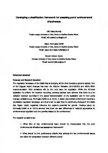
Figure 1: Application of normalization on log records

from the original Adaptive Semantic Filter is also used for the log normalization.

2.1.1

Log Message Normalization

As proposed by Liang et al. [2], log messages can be normalized by applying transformations that include the following steps: 1. Removing punctuation, e.g., . | < > +

; :

?

!

= - [ ]

2. Removing definite and indefinite articles, e.g., a, an, the 3. Removing weak words, e.g., be, is are, of, at, such, after, from 4. Replacing all numbers by the word NUMBER 5. Replacing all hex addresses with N digits by the word NDigitHex_Addr 6. Replacing domain specific identifiers by corresponding words such as REGISTER or DIRECTORY 7. Replacing all dates by DATE

Preprocessing

Log files of large systems usually contain huge amounts of log entries. However, many of the log entries contain redundant information, as a single root cause may trigger multiple components of the system to write log entries to the file. Moreover, the components may even produce different log messages for the same root cause. However, redundant log entries describe the same information and are not of interest for machine learning purposes. In order to remove redundant log events, we employ a combination of log message normalization and filtering, as detailed in Sections 2.1.1 and 2.1.2. The key idea behind the filtering is to remove redundant information by considering the time gap and the semantic correlation between two log records. For the filtering, we use the approach of Adaptive Semantic Filter by Liang et al. [2] and our Duplicate Removal Filter. A part 1

4 torus receiver x+ input pipe error(s) (dcr 0x02ec) 1 torus receiver x- input pipe error(s) (dcr 0x02ed) 191790399 L3 EDRAM error(s) (dcr 0x0157) detected 2 L3 EDRAM error(s) (dcr 0x0157) detected Error receiving packet, expecting type 57 3 torus receiver y+ input pipe error(s) (dcr 0x02ee) 3 torus receiver z- input pipe error(s) (dcr 0x02f1)

http://www.iste.uni-stuttgart.de/rss/people/pitakrat/scape

Figure 1 exemplifies the effect of applying the normalization. Six example log messages from the Blue Gene/L log, used in the evaluation, are shown in Figure 1a; the corresponding normalized messages are shown in Figure 1b. It is obvious that very similar log messages are mapped to the same normalized log message. This enables to programmatically grasp the semantic context of log messages as identical normalized log messages that are also mostly semantically identical.

2.1.2

Filtering

After the log is normalized by applying the aforementioned step, it can be processed by the filtering step, which removes redundant information. This section describes two types of filters used in this paper, namely Adaptive Semantic Filtering and Duplicate Removal Filtering.

Adaptive Semantic Filter. Liang et al. [2] propose a filtering algorithm, called Adaptive Semantic Filtering (ASF), which isolates important events in the Blue Gene/L log by removing redundant log entries. Log entries are considered redundant when they occur within a certain time frame and have a certain semantic correlation. The general idea behind ASF is that log records occurring close to each other in time most probably originate from the same root cause, even if the semantic correlation is not extraordinary high. On the other hand, log records with a larger time difference in between more probably originate from different root causes. Hence, the semantic correlation of two log records also needs to be higher in order to consider them to be redundant. To face this, ASF requires a higher semantic correlation of two log records if the time difference between them is greater than a certain threshold. To calculate the semantic correlation between two log entries, the log messages are first normalized, as described in Section 2.1.1 and then transformed into dictionaries of words. As the dictionaries are simply boolean vectors, similarity coefficients such as the Phi correlation coefficient can be used to compute the correlation. We denote cab ∈ N0 with a, b ∈ 0, 1 as the number of words that are not present in any of the two log messages (a = b = 0), that are only present in the first log message (a = 1, b = 0), that are only present in the second log message (a = 0, b = 1) and that are present in both log messages (a = b = 1). The Phi correlation coefficient is then defined as [2]:

c00 c11 − c01 c10 φ= p (c00 + c01 )(c10 + c11 )(c00 + c10 )(c01 + c11 )

(1)

The formula yields similarity coefficients between −1 to 1. The more similar two log messages are (high c00 or high c11 ), the closer the Phi correlation coefficient is to 1 and the more different two log messages are (high c01 or high c10 ), the closer the Phi correlation coefficient is to −1. The two messages that have a high coefficient are reduced to only one even though they occur far apart from each other. On the other hand, two messages that are less similar may be reduced if they occur close to each other.

Duplicate Removal Filter. The duplicate removal filter (DRF) is a filter that we have developed based on a straightforward idea: the log messages that have the same information and occur within a certain time span can be reduced to only one log record. This removal step aims to decrease the computation complexity of the Phi correlation coefficient, while still maintaining a high classification quality.

2.2

System Event Classification

The information contained in the log files can be used to conclude about the current state of the system, whether the system is running normally or it is experiencing a problem. Although the log messages may have certain formats or patterns, they usually differ across different parts or different versions of the system. Furthermore, log files can grow very large in complex systems which makes manual classification infeasible.

Our event classification approach is based on supervised machine learning which takes a set of manually labeled log messages as input to the algorithm. The algorithm learns an internal model, e.g., decision trees, data clusters, and probabilistic representations, from the data by discovering the patterns of log messages and the relationship to the given labels. After the model is trained, it is used to classify log messages that are produced at runtime and tag them with a label. Given the example in Figure 1a, the classification process starts by having a subset of the log manually labeled by the system administrators [5]. The labeled log is presented in Figure 2 where the labels are added to the beginning of the log messages. This example subset of log contains only two types of labels: “-” and “KERNREC” which implies that the machine learning model trained with this data will be able to classify and predict only two types of labels. At runtime, the unlabeled log messages are fed to the model which will classify them with the corresponding label. - 4 torus receiver x+ input pipe error(s) (dcr 0x02ec) - 1 torus receiver x- input pipe error(s) (dcr 0x02ed) - 191790399 L3 EDRAM error(s) (dcr 0x0157) detected - 2 L3 EDRAM error(s) (dcr 0x0157) detected KERNREC Error receiving packet, expecting type 57 - 3 torus receiver y+ input pipe error(s) (dcr 0x02ee) - 3 torus receiver z- input pipe error(s) (dcr 0x02f1)

detected detected

detected detected

Figure 2: Example of labeled log messages To give a concrete example, Table 1 provides all labels contained in the Blue Gene/L log file, which is used in the evaluation, with examples of log messages and statistics about the number of occurrences in the data. The events that are classified in this stage will serve as a basis for predicting future events described in the next section.

2.3

System Event Prediction

The idea of event prediction is based on an assumption that patterns in the event log can lead to certain events in the near future. Unlike event classification, which aims to classify a log message with a label, event prediction looks at the current sequence of messages and tries to predict if any type of event will occur soon. The training process of system event prediction starts by grouping a certain number of log messages from the past to the most recent one. Instead of taking the label of the current message for the training, we look ahead in time and take the label of the message in the future. However, predicting the occurrence of one label exactly at a specific time in the future is virtually impossible. This is because the predicted label may occur a few seconds earlier or later which makes our prediction a false positive. Therefore, we employ a prediction window where a prediction is regarded as correct if the predicted label occurs in this time window. Nonetheless, another issue remains in the consideration of the label as there can be many labels occurring in the prediction window. We solve this issue by dropping the type of the labels and consider a prediction as correct if there is at least a certain amount of any labels excluding “-” in that period. Figure 3 illustrates our prediction approach. The parameters that can be adjusted for event prediction are the number

Count 1 1 1 1 2 2 3 3 3 5 10 10 12 14 14 16 18 24 37 94 144 166 192 209 320 342 512 720 816 1503 1991 2048 2370 3983 5983 6145 23338 31531 49651 63491 152734 4399503

Label KERNBIT KERNEXT KERNTLBE MONILL LINKBLL MONNULL KERNFLOAT KERNRTSA MMCS KERNPROG APPTORUS MASNORM MONPOW KERNNOETH LINKPAP KERNCON KERNPAN LINKDISC MASABNORM KERNSERV APPALLOC LINKIAP KERNPOW KERNSOCK APPCHILD KERNMC APPBUSY KERNMNT APPOUT KERNMICRO APPTO APPUNAV APPRES KERNRTSP APPREAD KERNREC KERNTERM KERNMNTF APPSEV KERNSTOR KERNDTLB -

Message KERNEL FATAL ddr: redundant bit steering failed, sequencer timeout KERNEL FATAL external input interrupt (unit=0x03 bit=0x01): tree header with no target waiting KERNEL FATAL instruction TLB error interrupt MONITOR FAILURE monitor caught java.lang.IllegalStateException: while executing CONTROL Operation LINKCARD FATAL MidplaneSwitchController::clearPort() bll clear port failed: R63-M0-L0-U19-A MONITOR FAILURE While inserting monitor info into DB caught java.lang.NullPointerException KERNEL FATAL floating point unavailable interrupt KERNEL FATAL rts assertion failed: personality->version == BGLPERSONALITY VERSION in void start() at start.cc:131 MMCS FATAL L3 major internal error KERNEL FATAL program interrupt APP FATAL external input interrupt (unit=0x02 bit=0x00): uncorrectable torus error BGLMASTER FAILURE mmcs server exited normally with exit code 13 MONITOR FAILURE monitor caught java.lang.UnsupportedOperationException: power module U69 not present and is stopping KERNEL FATAL no ethernet link LINKCARD FATAL MidplaneSwitchController::parityAlignment() pap failed: R22-M0-L0-U22-D, status=00000000 00000000 KERNEL FATAL MailboxMonitor::serviceMailboxes() lib ido error: -1033 BGLERR IDO PKT TIMEOUT KERNEL FATAL kernel panic LINKCARD FATAL MidplaneSwitchController::sendTrain() port disconnected: R07-M1-L1-U19-E BGLMASTER FAILURE mmcs server exited abnormally due to signal: Aborted KERNEL FATAL Power Good signal deactivated: R73-M1-N5. A service action may be required. APP FATAL ciod: Error creating node map from file /p/gb2/draeger/benchmark/dat16k 062205/map16k bipartyz LINKCARD FATAL MidplaneSwitchController::receiveTrain() iap failed: R72-M1-L1-U18-A, status=beeaabff ec000000 KERNEL FATAL Power deactivated: R05-M0-N4 KERNEL FATAL MailboxMonitor::serviceMailboxes() lib ido error: -1019 socket closed APP FATAL ciod: Error creating node map from file /p/gb2/cabot/miranda/newmaps/8k 128x64x1 8x4x4.map KERNEL FATAL machine check interrupt APP FATAL ciod: Error creating node map from file /p/gb2/pakin1/sweep3d-5x5x400-10mk-3mmi-1024pes-sweep/sweep.map KERNEL FATAL Error: unable to mount filesystem APP FATAL ciod: LOGIN chdir(/p/gb1/stella/RAPTOR/2183) failed: Input/output error KERNEL FATAL Microloader Assertion APP FATAL ciod: Error reading message prefix on CioStream socket to 172.16.96.116:41739, Connection timed out APP FATAL ciod: Error creating node map from file /home/auselton/bgl/64mps.sequential.mapfile APP FATAL ciod: Error reading message prefix after LOAD MESSAGE on CioStream socket to 172.16.96.116:52783 KERNEL FATAL rts panic! - stopping execution APP FATAL ciod: failed to read message prefix on control stream CioStream socket to 172.16.96.116:33399 KERNEL FATAL Error receiving packet on tree network, expecting type 57 instead of type 3 KERNEL FATAL rts: kernel terminated for reason 1004rts: bad message header KERNEL FATAL Lustre mount FAILED : bglio11 : block id : location APP FATAL ciod: Error reading message prefix after LOGIN MESSAGE on CioStream socket KERNEL FATAL data storage interrupt KERNEL FATAL data TLB error interrupt KERNEL INFO instruction cache parity error corrected

Table 1: Statistics and example of log file collected from Blue Gene/L

of past observations to be taken into account, how long we look into the future (lead time), the length of the prediction window, and the percentage of the messages that have to be labeled with a fault state so that a failure should be predicted in this timeframe (sensitivity). Observation window

x

x

x

Lead time

stead. Assume that the prediction window is two messages ahead in the future and contains two messages which are: KERNREC Error receiving packet, expecting type 57 - 3 torus receiver y+ input pipe error(s) (dcr 0x02ee) detected

Prediction window

x

x

If we set the sensitivity to 50%, the first group of messages will be labeled as a “+” as it contains at least 50% of the messages not labeled with “-”.

Figure 3: Timeline of system event prediction Using the example in Figure 1a for the illustration, the training phase groups a certain number of log messages together. Assume that the number of past observation is three, three consecutive log messages will be grouped as one entry. Figure 4a shows the first group of log messages. The next group of messages is obtained by sliding the observation window to the next message which is shown in Figure 4b. 4 torus receiver x+ input pipe error(s) (dcr 0x02ec) detected 1 torus receiver x- input pipe error(s) (dcr 0x02ed) detected 191790399 L3 EDRAM error(s) (dcr 0x0157) detected

(a) First group of log messages 1 torus receiver x- input pipe error(s) (dcr 0x02ed) detected 191790399 L3 EDRAM error(s) (dcr 0x0157) detected 2 L3 EDRAM error(s) (dcr 0x0157) detected

(b) Second group of log messages

Figure 4: Example of grouped log messages As we are predicting whether there will be any label occurring in the near future, we neglect the label of those messages in the group and take the label of the future messages in-

On the other hand, the prediction window of the second group of log messages will also slide to the next message and contain: - 3 torus receiver y+ input pipe error(s) (dcr 0x02ee) detected - 3 torus receiver z- input pipe error(s) (dcr 0x02f1) detected

The second group of messages will be labeled as a “-”, as this prediction window does not contain any label other than “-”. This grouping process continues for the remaining part of the available log. When all log messages are processed, the grouped and labeled entries are used for training the model. At runtime, the new log messages are grouped according to the configured parameters and fed to the trained model which predicts the future event for that group.

3.

FRAMEWORK ARCHITECTURE

We developed a framework that implements our event classification and prediction approach. The framework is written in Java and is built on the Kieker monitoring framework [11]. The Kieker’s pipe-and-filter architecture provides the flexibility to handle variable input and output interfaces. This

allows our framework to analyze both log files in offline mode to evaluate the quality of machine learning algorithms, and to predict upcoming failures in running software systems. As illustrated in Figure 5, the framework consists of a set of interconnected filters that process streams of incoming log messages. The filters serve for preprocessing, labeling, shuffling, evaluation, training, and prediction. The filters allow for both event classification and prediction, and are detailed below. Log message

Evaluation Filter. The evaluation filter collects the preprocessed data from previous filters and splits them into ten parts. It then executes the 10-fold cross-validation by directing the data to the training and prediction filters and collects the results.

4.

• RQ1: How do different machine learning algorithms perform for system event classification and prediction?

Preprocessing Filter

• RQ2: What is the impact of log filtering on the size of the dataset and on the classification quality?

Labelling Filter

Shuffling Filter

Evaluation Filter

EVALUATION

This section describes the evaluation of the approach applied to a publicly available log file collected from a supercomputer at Sandia National Laboratories [5].2 Our evaluation aims to answer the following research questions:

Classification and prediction results

In Section 4.1 we describe the details of the dataset used in the evaluation. Section 4.2 explains the methodology of the evaluation. Section 4.3 presents the results of event classification and prediction in order to answer RQ1 and RQ2.

4.1 Training Filter

Prediction Filter

Figure 5: Architecture overview of SCAPE

Preprocessing filter. The preprocessing filter includes all the functionalities described in Section 2.1. The filter can be configured to apply different combinations of the described preprocessing steps. For example, it can be set to only normalize the log, normalize and apply ASF, or normalize and apply DRF.

Labeling filter. This filter takes care of re-arranging the log messages and labeling them to align with the corresponding approach. If the purpose of the execution is to classify the messages, the messages will be tagged with their original labels. On the other hand, if it is predicting the future event, messages will be grouped together and will be assigned the label that occurs in the future.

Shuffling filter. The shuffling filter uses stratified sampling to change the order of the messages in the log file. Its purpose is to distribute all types of messages equally over the dataset which increases the stability of the evaluation over different parts of the log file.

Training Filter. The training filter is responsible for training the classification and prediction models by taking the log messages and the labels as input. The output of this filter is a machine learning model which is ready to be used for both classifying or predicting future events.

Prediction Filter. The prediction filter receives the unlabeled log messages collected at runtime as input as well as the models obtained from the training filter. The output of the prediction filter are the labels of the input messages.

Dataset

The dataset used in the evaluation is a log file which contains 215 days of log messages generated by a Blue Gene/L supercomputer system, which has 131,072 processors and 32,768 GB of RAM [5]. Each message contains the category (label), the timestamp (GMT), the date, the name of the device, and the actual message. The category or label of each message is identified and added by the system administrator. It indicates the type of the alert that the respective message represents. As presented in Table 1, there are 42 types of labels in total, including the empty label.

4.2

Methodology

The log file of Blue Gene/L contains a large number of log messages and all of the data cannot be processed at once in the evaluation. We, thus, split the log file into blocks where each block contains approximately the same number of log messages. However, the log messages are not generated uniformly over the time, i.e., some types of messages may occur more often at the beginning of the file and vice versa. If the blocks are split by the temporal ordering of the messages, the non-uniform distribution can affect the evaluation since some types of messages may not occur in some blocks. Therefore, we used stratified sampling to maintain the proportion of the types of messages in all blocks. The machine learning library used in our evaluation is Weka [1]. It provides many machine learning algorithms. In order to determine the classification quality, we use the common approach of 10-fold cross-validation which splits the data of each block into 10 parts and uses 9 parts for training the model and 1 part for the validation. The validation is repeated 10 times and the final result is obtained by averaging the results of all runs. We used the standard metrics, such as, true/false positive/negative rates, to evaluate the experiment results. The detailed description of these metrics can be found in [10]. 2

http://www.cs.sandia.gov/˜jrstear/logs/

FMeasure of all labels

Results

1.0

4.3.1

● ●

This section presents the results of the evaluation, addressing the previously mentioned research questions.

0.8 FMeasure

4.3

0.4 0.2

Quality of System Event Classification

● ● ● ●

0.0

− APPALLOC APPBUSY APPCHILD APPOUT APPREAD APPRES APPSEV APPTO APPTORUS APPUNAV KERNCON KERNDTLB KERNFLOAT KERNMC KERNMICRO KERNMNT KERNMNTF KERNNOETH KERNPAN KERNPOW KERNREC KERNRTSP KERNSOCK KERNSTOR KERNTERM LINKDISC LINKIAP MASABNORM MMCS MONNULL MONPOW

For event classification, we selected two attributes of the log messages and used them to train the models. These attributes are the label and the actual message of the log. The other attributes, such as, timestamp, location, are neglected as they are independent and do not contribute to the assignment of the label of the message.

FMeasure of all labels (a) Naive Bayes with original log 1.0 ● ●

FMeasure

● ●

●

0.8 0.6

● ●

●

●

0.4

●

0.2 − APPALLOC APPBUSY APPCHILD APPOUT APPREAD APPRES APPSEV APPTO APPTORUS APPUNAV KERNCON KERNDTLB KERNFLOAT KERNMC KERNMICRO KERNMNT KERNMNTF KERNNOETH KERNPAN KERNPOW KERNREC KERNRTSP KERNSOCK KERNSTOR KERNTERM LINKDISC LINKIAP MASABNORM MMCS MONNULL MONPOW

Figure 6 illustrates the precision and recall of classifying the label KERNMNTF over 19 blocks. The log file is split into blocks using stratified sampling and normalized according to Section 2.1.1. It can be seen from both plots that precision and recall are similar in all blocks. This result concludes that the log file can be split and evaluated separately without Precision of Label Recall of Label significant deviation between blocks. KERNMNTF KERNMNTF

0.6

FMeasure

0.8 0

3

6

9

13

17

Block

(a) Precision

0

3

6

9

13

17

Block

(b) Recall

Figure 6: Precision and recall of KERNMNTF label using naive Bayes on normalized log file Figure 7 illustrates the F-measure of three configurations of event classification, namely (i.) naive Bayes without normalization, (ii.) naive Bayes with normalization, and (iii.) C4.5 with normalization. Figure 7a is the result of applying naive Bayes on the original unfiltered log messages. As the log file is not normalized, the messages contain noise from the numerical values, weak words, etc. This noise results in the highly varying F-measure across different labels. Figures 7b and 7c illustrate the F-measure of classification using naive Bayes and C4.5 on the normalized log file. The results show significant improvements of all labels over the original log file and, on average, C4.5 performs better than naive Bayes. Specifically, the number of labels for which naive Bayes has a recall of zero—leading to an undefined F-measure—is considerably higher than for C4.5. From the classification results, we can conclude that log normalization helps increase the classification quality as the noise in the messages are filtered out. Moreover, C4.5 outperforms naive Bayes with F-measure values of 1 for classifying most of the labels.

4.3.2

Impact of Log Filtering

Figure 8 shows the number of log messages with INFO severity plotted according to their temporal position in the log file. By comparing the y-axis of the plots, it can be observed that there is a significant reduction in the number of peaks of similarly labeled records located close to each other. Whilst in hour 2,932 there are more than 130,000 log

●

● ● ●

●

● ● ●

●

●

− APPALLOC APPBUSY APPCHILD APPOUT APPREAD APPRES APPSEV APPTO APPTORUS APPUNAV KERNCON KERNDTLB KERNFLOAT KERNMC KERNMICRO KERNMNT KERNMNTF KERNNOETH KERNPAN KERNPOW KERNREC KERNRTSP KERNSOCK KERNSTOR KERNTERM LINKDISC LINKIAP MASABNORM MMCS MONNULL MONPOW

0.0

0.4

Recall

0.8 0.4 0.0

Precision

FMeasure all labels (b) Naive Bayes withofnormalized log 1.00 0.95 0.90 0.85 0.80 0.75 0.70

(c) C4.5 with normalized log

Figure 7: F-measure of event classification using different algorithms

records with INFO severity–after filtering there remain only less than 30 for ASF and 400 for tuned ASF and DRF. This shows that the filters are capable of effectively eliminating large amounts of redundant log records that occur close to each other. To evaluate the impact of the log filtering on the event classification, the ASF and DRF techniques (see Section 2.1.2) are applied to the log messages to produce a reduced set of log records. The log messages that are the output of the filters are used as a training set of the machine learning algorithms. Once the algorithms are trained, the classification is done on the original set of log messages excluding those that are used in the training. It is important to note that—as the log file is large—the log messages are split into blocks where each block contains 500,000 log messages and the evaluation is carried out for every block. The impact of the filtering on the system event classification is depicted in Figure 9. The first and the second boxes show the F-measure of the original ASF and the ASF that is tuned to produce the best result. The third box shows the F-measure when applying DRF. It can be seen that the F-measure of the tuned ASF and DRF are approximately the same but are slightly higher than the original ASF. This result concludes that, although the tuned ASF and DRF perform better than the original ASF, the improve-

20 10 0

40000

Amount

30

100000

Amount of Label INFO

0

Amount

Amount of Label INFO

0

500

1500

2500

0

3500

1500

2500

3500

(b) Original ASF

(a) Original log

Amount of Label INFO

200

Amount

100

0

0

100

300

300

Amount of Label INFO

Amount

500

Time after startup [h]

Time after startup [h]

0

500

1500

2500

3500

Time after startup [h]

0

500

1500

2500

3500

Time after startup [h]

(c) Tuned ASF

(d) DRF

Figure 8: Number of messages with INFO severity before and after applying different filters ment is not quite significant. Moreover, the tuned ASF is specifically adjusted for this set of data and may not produce as good result for log files collected from other systems. Nonetheless, DRF which we developed proves to be as effective as the tuned ASF in filtering out the redundant log messages with less computational complexity.

Table 2c shows the resulting F-measures for prediction windows from 60 to 4,800 seconds with 3 past observations, lead time of 600 seconds, and sensitivity at 20%. It is obvious that the longer the prediction window, the better the F-measure as the longer window covers a longer time span which increases the chance of including more events in that period. However, there is a trade-off between prediction accuracy and the significance of the prediction as the longer the prediction window is, the less useful it becomes. Therefore, the selection of the prediction window is context-dependent and needs to be adjusted according to the target system. The last parameter of the prediction is the sensitivity. The result is shown in Table 2d. The best sensitivity for naive Bayes is 1% while C4.5 performs best with 40%. It is worth noting that, the higher the sensitivity, the lower the Fmeasure. The reason is because higher sensitivity means more log messages have to have labels other than “-”. This is especially difficult if the sensitivity is 100% which means there can be no “-” label in the prediction window.

0

0.95

0.96

0.97

0.98

0.99

1.00

In conclusion, the parameters that result in a similar effect for both algorithms are the lead time and the length of the prediction window. The smaller the lead time, the better the accuracy as it is easier to make predictions in the near future than further away in time. Likewise, the longer the prediction window, the better the accuracy as it increases the chance of events occurring in that time span.

Original ASF

Tuned ASF

DRF

Figure 9: F-measure of event classification when applying different filters

4.3.3

Table 2b presents the resulting F-measures when the lead time varies from 0 to 2,800 seconds with 3 past observations, a prediction window of 600 seconds, and sensitivity at 20%. From the table, we can observe that the lead time of 0 seconds has the best F-measure. In other words, our prediction is most accurate when the prediction window starts right after the observation window.

Quality of System Event Prediction

The system event prediction described in Section 2.3 has a number of parameters. These parameters are evaluated individually by varying the value of one parameter while fixing the others. We experimented with various machine learning algorithms, e.g., naive Bayes, C4.5, Random Forest, RepTree, K*, K-nearest neighbours on the normalized log messages and filtered by DRF. The preliminary results show that the naive Bayes and C4.5 outperform the others. Hence, the following results are the experiment of naive Bayes and C4.5 as the exhaustive experiment of all algorithms with all configurations is computationally expensive and infeasible.

On the other hand, the number of past observations and the sensitivity show opposite effects on the two algorithms. While the higher number of past observations reduces the accuracy of naive Bayes, it increases the accuracy of C4.5. However, in this case, the effect of the sensitivity does not seem to be correlated with the prediction accuracy and, therefore, should be adjusted specifically per application. Algorithm 1 0.603 0.621

NaiveBayes C4.5

Number of past observations 3 4 6 8 0.506 0.500 0.501 0.501 0.624 0.624 0.624 0.626

16 0.503 0.634

(a) Different number of past observations Algorithm NaiveBayes C4.5

0 0.663 0.877

60 0.589 0.672

Lead 120 0.547 0.634

time (sec) 300 600 0.517 0.506 0.627 0.624

1200 0.511 0.640

2800 0.506 0.625

(b) Different lead time Algorithm NaiveBayes C4.5

Table 2a shows the resulting F-measures for predicting the future event when the number of past observations is varied from 1 to 16. For this configuration, the lead time and the length of the prediction window are set to 600 seconds, and the sensitivity is set to 20%. From the table, naive Bayes appears to have the highest F-measure when taking into account only one past observation while the C4.5 has the highest F-measure with 16 past observations.

2 0.517 0.626

60 0.491 0.579

120 0.493 0.578

Prediction window (sec) 300 600 1200 0.485 0.506 0.511 0.598 0.624 0.640

2800 0.532 0.625

4800 0.553 0.635

(c) Different prediction window Algorithm NaiveBayes C4.5

1% 0.546 0.523

5% 0.522 0.572

10% 0.516 0.609

Sensitivity 20% 40% 0.506 0.462 0.624 0.691

80% 0.519 0.234

100% 0.399 -

(d) Different sensitivity

Table 2: F-measures of system event prediction with different parameter configurations

5.

RELATED WORK

The comprehensive analysis of log files collected from supercomputers was investigated by Oliner and Stearley [5] where the authors inspect the characteristics of the log and the challenges to identify alerts in five different high performance computing (HPC) systems. The authors further introduce an approach called NodeInfo to detect alerts in the log using an unsupervised algorithm for anomaly detection [6]. The goal of the work was to identify the regions in the log file in which the alerts occur. Zheng et al. [14] propose an approach to predict failures and their locations in the Blue Gene/P supercomputer. The approach employs genetic algorithms to generate rules that can best represent the log pattern preceding failures. Yu et al. [13] compares two widely-used approaches, which are period-based and event-based, to predict failures in Blue Gene/P. A Bayesian prediction model is used to evaluate the accuracy of both methods and the results show that the event-based approach outperforms the period-based approach. Liang et al. [3] split log files into windows and extract the statistics of events into features. Different machine learning algorithms are then applied to learn the extracted features and predict whether a failure is pending. Xu et al. [12] detect problems in large-scale systems by combining source code analysis with machine learning to mine composite features and detect operational problems at runtime. Nakka et al. [4] predicts node failures in HPC systems by analyzing many parameters, such as, time of usage, system idle time, etc., and applying a decision tree classifier to predict a failure within the next one hour. Salfner [9] employs and extends the traditional hidden Markov models to predict failures based on the event log of a telecommunication system. Our approach takes a new direction by classifying messages using supervised machine learning algorithms. Based on the classified messages, we predict the events that can occur in the near future. The prediction provides useful information and warnings to the system administrators to initiate countermeasures in advance before the problems actually arise.

6.

CONCLUSION

Software systems in production produce large event logs with messages of different severity from different sources. The data contain important information to diagnose system failures but processing these data is a big challenge. In this paper, we presented our SCAPE approach for automatic classification and prediction of event log. A proof-of-concept implementation is provided in form of a reusable and extensible framework, which is part of our Hora online failure prediction approach. We evaluated our approach by applying it to a large, publicly available event log of a Blue Gene/L supercomputer. The evaluation results revealed a high classification quality and showed promising initial results for the event prediction. In our future work, we will focus on the improvement of the prediction quality of individual labels. Moreover, as part of the overall Hora vision [8], we will combine the event log analysis with other quality-of-service evaluation techniques available in the Hora framework, e.g., time series analysis, to extend its online failure prediction capability.

References [1] G. Holmes, A. Donkin, and I. Witten. Weka: a machine learning workbench. In Proc. 2nd Australian and New Zealand Conf. on Intelligent Information Systems, pages 357 –361, 1994. [2] Y. Liang, Y. Zhang, H. Xiong, and R. K. Sahoo. An adaptive semantic filter for Blue Gene/L failure log analysis. In Proc. Int’l Parallel and Distributed Processing Symp., pages 1–8, 2007. [3] Y. Liang, Y. Zhang, H. Xiong, and R. K. Sahoo. Failure prediction in IBM BlueGene/L event logs. In Proc. 7th IEEE Int’l Conf. on Data Mining, pages 583–588, 2007. [4] N. Nakka, A. Agrawal, and A. Choudhary. Predicting node failure in high performance computing systems from failure and usage logs. In Proc. IEEE Int’l Symp. on Parallel and Distributed Processing Workshops and Phd Forum, pages 1557–1566, 2011. [5] A. Oliner and J. Stearley. What supercomputers say: A study of five system logs. In Proc. 37th Annual IEEE/IFIP Int’l Conf. on Dependable Systems and Networks, pages 575–584, 2007. [6] A. J. Oliner, A. Aiken, and J. Stearley. Alert detection in system logs. In Proc. 8th IEEE Int’l Conf. on Data Mining, pages 959–964, 2008. [7] T. Pitakrat. Hora: Online failure prediction framework for component-based software systems based on Kieker and Palladio. In Proc. Symp. on Software Performance: Joint Kieker/Palladio Days, 2013. [8] T. Pitakrat, A. van Hoorn, and L. Grunske. Increasing dependability of component-based software systems by online failure prediction. In Proc. 10th European Dependable Computing Conf., pages 66–69, 2014. [9] F. Salfner. Event-based Failure Prediction: An Extended Hidden Markov Model Approach. PhD thesis, Humboldt-Universit¨ at zu Berlin, 2008. [10] F. Salfner, M. Lenk, and M. Malek. A survey of online failure prediction methods. ACM Computing Surveys, 42(3):10:1–10:42, 2010. [11] A. van Hoorn, J. Waller, and W. Hasselbring. Kieker: A framework for application performance monitoring and dynamic software analysis. In Proc. 3rd ACM/SPEC Int’l Conf. on Performance Engineering, pages 247– 248. ACM, 2012. [12] W. Xu, L. Huang, A. Fox, D. Patterson, and M. I. Jordan. Detecting large-scale system problems by mining console logs. In Proc. ACM SIGOPS 22nd Symposium on Operating systems Principles, pages 117–132, 2009. [13] L. Yu, Z. Zheng, Z. Lan, and S. Coghlan. Practical online failure prediction for Blue Gene/P: period-based vs event-driven. In Proc. Int’l Conf. on Dependable Systems and Networks Workshops, pages 259–264, 2011. [14] Z. Zheng, Z. Lan, R. Gupta, S. Coghlan, and P. Beckman. A practical failure prediction with location and lead time for Blue Gene/P. In Proc. Int’l Conf. on Dependable Systems and Networks Workshops, pages 15–22, 2010.