A Framework for Dynamic Resource Assignment and Scheduling on ...

A Framework for Dynamic Resource Assignment and Scheduling on Reconfigurable Mixed-Mode On-Chip Multiprocessors Xiaofang Wang and Sotirios G. Ziavras Department of Electrical and Computer Engineering New Jersey Institute of Technology Newark, NJ 07102, USA {xw23, ziavras}@njit.edu

Abstract Encouraged by continuous advances in FPGA technologies, we explore high-performance MultiProcessor-on-a-Programmable-Chip (MPoPC) reconfigurable architectures. This paper proposes a methodology for assigning resources at run time and scheduling large-scale floating-point, data-parallel applications on our mixed-mode HERA MPoPC. HERA stands for HEterogeneous Reconfigurable Architecture. An application is represented by a novel mixed-mode task flow graph which is scheduled to run under a variety of independent or cooperating parallel computing modes: SIMD (Single-Instruction, Multiple-Data), Multiple-SIMD and MIMD (Multiple-Instruction, Multiple-Data). The reconfigurable logic is customized at static time and reconfigured at run time to match application characteristics. An in-house developed parallel power flow analysis code by Newton s method is employed to verify the methodology and evaluate the performance. This application is of utmost importance to any power grid.

1. Introduction The recent capabilities of state-of-the-art FPGAs in terms of resources and speed provide new opportunities in reconfigurable computing. The peak performance of individual floating-point (FP) operations on FPGAs has outnumbered in the last few years that of modern microprocessors and is growing faster than the latter [1]. Recent relevant work [2-4] further confirms and strengthens this trend. It is viable now for FPGAs to accommodate complex high-performance applications. Encouraged by continuous advances in FPGA technologies, we explore high-performance cluster-on-a-chip (i.e., MPoPC) reconfigurable architectures for large-scale computation-greedy, data-parallel applications. These applications often involve complex matrix-based algorithms where software programmability and standard FP representation are indispensable. _______________________________ *This work was supported in part by the U.S. Department of Energy under grant DE-FG02-03CH11171.

Scalability and portability are also essential to performance due to the variant size of matrices and the ever changing parameters of various applications. Compiling tools for FPGAs targeting spatial computing from high-level descriptions, such as C/C++, Java and Matlab [e.g., 9-13], are emerging to deal with challenges in multi-million-gate FPGA designs. FPGA-based systems have enjoyed great success in accelerating many computation-intensive applications due to their superior resource utilization [5-6]. However, most often reconfigurable computing systems are application-specific programmable circuits (ASPCs) tailored to a particular algorithm. Therefore, they are developer programmable rather than user programmable. If the design size overflows the resources, which is often the case for matrix-based applications, device reprogramming is required; it usually takes tens to one hundred milliseconds and may have an adverse effect on the execution time. This issue becomes more serious with increases in the chip size [7] because the size of configuration data is proportional to the total number of on-chip resources. Also, the time-consuming hardware design and implementation procedure has to be repeated every time a change is made to the source code. Our solution is based on user programmable MPoPCs that support partial runtime reconfiguration. In addition to alleviating the above difficulties, MPoPCs can offer several advantages for our target applications. Medium- to coarse-grain modular architectures (e.g., XPP [8]) are simpler and more scalable than complex custom designs. Hence, MPoPCs can potentially achieve higher system frequencies than the latter. This feature also reduces the verification time, which is a major part of current deep-submicron designs. The communication latencies in MPoPCs can be very low. They also have lower cost and design risk compared to their ASIC peers. Another benefit is that we can leverage tremendous research results in computer architecture and parallel processing, and also incorporate reconfiguration. More importantly, we can customize the hardware architecture based on application characteristics and, hence, achieve a higher utilization of hardware resources compared to

1

systems with general-purpose microprocessors or ASICs. This paper proposes a framework for mapping, scheduling and executing applications with large data sets on HERA [22], a mixed-mode MPoPC that we have designed and implemented on Xilinx Virtex II FPGAs. HERA can be reconfigured at run time to support a variety of independent or cooperating parallel computing modes, such as SIMD, MultipleSIMD and MIMD to match the unique requirements of applications. Not only does our approach exploit mixed-mode parallelism but we also put a major effort on effective resource management at both static and run time. A mixed-mode Task Flow Graph is constructed for a given application; tasks are classified according to their appropriate computing mode. A parameterized hardware component library (PHCL) is adopted to customize individual components in HERA configurations based on task requirements. During the execution of an application, we reallocate on-the-fly the required number of processors with appropriately reconfigured units to tasks based on the system status. An in-house developed parallel power flow analysis code for Newton s method [19] is employed to verify the methodology and evaluate the performance. Realtime solutions to this problem are of paramount importance to any power grid [18]. The remainder of the paper begins with an introduction of the key architectural features in HERA. Section 3 presents an overview of our framework. Section 4 focuses on task profiling. The architecture synthesis and reconfiguration scheme are presented in Section 5. Section 6 is devoted to the integrated dynamic resource scheduling and task execution process. The application study can be found in Section 7 and the conclusions in Section 8.

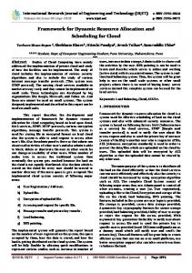
2. HERA: a Mixed-Mode MPoPC HERA targets matrix-based applications with large data sets. The general organization of our HERA machine with m x n PEs interconnected via a 2-D mesh network is shown in Figure 1. We employ fast, direct NEWS (North, East, West and South) connections for communications between nearest neighbors. Every column has a Cbus and all the Cbuses are connected to the Column Bus for broadcasting SIMD instructions and their data. The computing fabric is controlled by the system Sequencer that communicates with the host processor via the PCI bus for data I/O. The Global Control Unit (GCU), included in the system Sequencer, fetches instructions from the global program memory (GPM) for PEs operating in SIMD. A PE of HERA is an inhouse designed RISC processor built around a 7stage pipelined FPU with dual-port local data memory (LDM) and local program memory (LPM). The sizes of LPM and LDM are also determined

during the architecture synthesis stage. A novel feature of HERA s memory hierarchy is that the B port of every PE is shared with the neighbors to the south and east. A PE can directly write to or read from the LDMs of its west and north neighbors via their B ports. This feature can be used to eliminate omnipresent large block data transfers between nearest neighbors in numerous block-based matrix computations (e.g., LU factorization). HERA s modular instruction set contains about 30 instructions classified in six major groups: integer arithmetic, FP arithmetic, memory access, jump and branch, PE NEWS communications and system control. The operating mode of each PE can be configured dynamically by the host processor through its Operation Mode Register by using a Configure instruction. Combined with the PE ID number and masks, the system can be configured dynamically into a mixed-mode computing system capable of supporting simultaneously SIMD, MIMD and multiple-SIMD.

Figure 1. HERA organization.

3. Framework Overview Assume a matrix-based FP application and a programmable chip that supports run-time reconfiguration. The latter has the following available resources: (logic resources expressed in logic cells) and (total memory capacity expressed in bits), Our objective is to maximize resource utilization in the reconfigurable logic and potentially minimize the totaln execution time of the overall application, Ttotal i 1 T (i) , where T(i) is the execution time of task Si (all tasks in the application are considered). Figure 2 shows the general architecture of our framework for heterogeneous MPoPCs like HERA. There are five major phases in this framework: task profiling, system synthesis, task coding using the target system s instruction set, system implementation on FPGAs, and dynamic, simultaneous resource-efficient task decomposition,

2

mapping, scheduling and execution. The implementation on FPGAs follows the same procedure as any VHDL-based design methodology. Due to limited space, we focus on task profiling, system synthesis, and dynamic resource management and mapping, scheduling and execution.

4. Task Characterization A typical data-parallel FP application in engineering and science consists of blocks of nested loops which consume most of the overall execution time; these loops are controlled by conditional statements. In our framework, the behavioral description of the application is first analyzed to construct a Task Flow Graph (TFG), G = (S, D); it is a weighted, directed acyclic graph (wDAG). S and D represent the sets of nodes and edges, respectively. Figure 3 shows a typical TFG. Each node in this graph represents a task Si S, where i [1, n] is inclusive of all the tasks. There are two types of tasks: SIMD tasks (denoted by circles) and MIMD tasks (denoted by octagons). Associated with each task Si are its computing mode (SIMD/MIMD), FP computation number and FP operation types, represented by (Si), FP(Si) and (Si), respectively. The memory requirements (in bits) of each task are represented by two parameters, c(Si) and d(Si), for the instruction memory and data memory, respectively. A directed edge between two tasks Si and Sj represents a data dependence between them and its weight Di,j D represents the volume of data in bits that goes from task Si to Sj. An entry task is defined as a node with no incoming edges (e.g., S1 in Figure 3) and an exit task is defined as a node with no outgoing edges (e.g., S8). The selection of an optimal mode for each task can be a complex procedure and is not the focus of this paper. An SIMD task in our study is typically a data-parallel block (e.g., a nested loop) which can benefit from synchronous execution under SIMD, while an MIMD task is more of the control-flow style.

5. Architecture Synthesis and Reconfiguration In our framework, dynamic reconfiguration of computing resources for a given application is employed since FP computing cores are very resource expensive. Only the required FP operations are supported each time by PEs. The functionality of PEs can be changed via hardware reconfiguration at run time, as needed by the tasks.

5.1. Parameterized Hardware Component Library (PHCL) PHCL plays a major role in our methodology. The performance of the included components, in terms of speed and resource requirements, is

Figure 2. Framework overview/flowchart.

Figure 3. A typical task flow graph. manipulated in our approach. All the components are designed and compiled in VHDL. The major parameterized components for our matrix-based applications include: Variable precision pipelined FP function cores (including IEEE-754 single- and double-precision implementations, and other non-IEEE custom formats). Figure 4 shows the block diagram of an FP core whose major parameters are listed in Table 1. The cores are parameterized by the mantissa and exponent sizes. Different choices for the mantissa and exponent lead to different data ranges and resource requirements. Since FP cores are the main consumers of logic resources and embedded DSP cores in FPGAs, it is very important to choose the appropriate precision for the function cores. HERA architecture templates. Memory blocks, including single- and dual-port memories.

3

Custom function units, such as trigonometric function implementers. Various registers. Integer function cores parameterized by word size.

Figure 4. Block diagram of an FP core. Table 1. PHCL parameters of the FP core in Figure 4 Function

FP division

Mantissa (bits) Exponent (bits) Latency (cycles) Frequency(MHz) Logic resources (slices) Embedded DSP blocks Memory blocks (BRAM) Target device

24 8 27 189 979 None None Virtex II XC2V6000-5

among all paths, S1 S3 S5 forms the critical path in the TFG of Figure 5.a; also an FP divider is required by S3 which is a large task based on its number of FP operations. In this case, an FP divider is initiated for all PEs at the very beginning. B. Small tasks appear in the critical path. S5 in Figure 5.b is such an example. Because S3 is the task that potentially contributes the most to the execution time, the priority is to maximize the number of PEs for S3 with the inclusion of an FP adder and a multiplier as well. None of the PEs contains an FP divider until the execution of S5. Some PEs will be reconfigured to add an FP divider when the time comes for S5. C. Tasks are not in the critical path. This case is treated similarly to Case B. For example, an FP divider is added to some PEs at the time needed to accommodate task S4 shown in Figure 5.c.

5.2. System Synthesis The architecture generator takes a TFG and generates the initial architecture based on the computation types and amounts in tasks. A system template in VHDL is selected first from PHCL, with the basic PE interconnection and interface to the sequencer. We assume that the requirements of this template for logic resources and memory blocks are known as Lsys(p) in logic cells and Msys(p) in bits, for a given number of PEs p. The PE datapath (functionalities and width), total number of PEs and layout of PEs are customizable. The system generator first analyzes the data range of the application and decides on an appropriate precision for the FP cores. The total number of PEs is largely determined by this choice. Only the required function cores are included in PEs. It is possible that all the operation types are required throughout execution but only one or two operations are needed for a few tasks. For example, FP division is less frequent than multiplication and addition in many data-parallel applications. Based on our implementation results, a single-precision IEEE754 FP divider is at least more than two or five times larger in space than an FP adder or multiplier, respectively. These numbers are even larger for a double-precision FP divider. For less frequently used operations, we consider the following cases. An FP divider is used as an example. A. Large tasks appear in the critical path. A critical path in a TFG is a group of dependent tasks forming a linear array that comprises an entry task and an exit task, and has the largest number of FP operations and communication volume among all paths. It potentially determines the execution time of the entire application. Several algorithms exist in the literature to find such a path [14]. For example,

a b c Figure 5. Example of PE function selection. These decisions are based on our adaptive parallelization technique and the device reconfiguration latencies. We could make a more accurate decision by only adding an FP divider to some PEs just when needed. However, the device reconfiguration time of modern FPGAs is still significant and there is no sign that it will be reduced significantly in the near future. It may have an adverse effect if we either reprogram fully the chip or a large number of PEs required by large tasks. Thus, we are mainly interested in the partial runtime reconfiguration (PRTR) of FPGAs when no computation can be scheduled on some PEs while the remaining PEs are still busy with assigned tasks. Let p be the total number of PEs that can be implemented in the system and PEi requires L(i) logic resources. Also, the capacity of the instruction and data memories of each PEi is Mc(i) and Md(i), respectively. The following equations represent the objective functions in the recursive minimization procedure of our proposed system synthesis. p

L sys

L (k ) k 1 p

M sys

{M c(k )

M d ( k )}

k 1

4

6. Dynamic Resource Assignment and Task Scheduling This section discusses our Critical-Path driven maximum Resource Utilization dynamic Scheduling (CP-maxRUS) heuristic. Based on various application scenarios, system architectures and performance objectives, extensive scheduling research targeting multiprocessors has been done for fixed parallel architectures [14-15]. Scheduling is an NP-complete problem and a good heuristic for suboptimal performance should be the goal. There are more key features that distinguish our strategy from existing approaches. First, we target a real reconfigurable system under various resource constraints. Second, we explore adaptive parallelization of tasks; i.e., we determine the appropriate number of PEs and the binding of tasks to PEs at run time instead of making static decisions. Third, our adaptive parallelization is PE-oriented rather than task-oriented.

6.1. Loop Partitioning

Then the above partitioning techniques can be applied to these loops. Other loops that can be transformed into FOR loops (e.g., WHILE loops) are treated similarly.

6.2. PE Searching The order in which we search for candidate PEs is an important step affecting the overall mapping performance. Based on HERA s organization and interconnection network, we propose our PULSE column-biased search process that uses the pattern since the distance between two adjacent stops in this search pattern is always one. Another reason is one port of the data memory of each PE is shared with its immediate neighbors to the west and south. Assume that the numbers of PEs assigned concurrently to tasks Si and Sj are pi and pj, respectively, and x = min{pi, pj}. The objective function to be minimized in this step is the communication time among tasks n , where Dij is Tcom

max{[ Dij /( * x) Tini ] * H (i, j ) Tcflit}

i, j 1

Loop-based partitioning is the basis of our adaptive parallelization. We restrict our effort to assigning each time the complete or part of an iteration to a PE. Hence, flow dependence is allowed inside an assigned iteration. A. FOR loops without cross-iteration dependence Assume that the total number of PEs available to the loop is and the total number of iterations is L. The loop space is split into groups of size L / or L/

. Each PE gets such a group and the

corresponding data set. These loops map naturally to the SIMD mode and no communication is required. FOR loops without both flow dependence and crossiteration dependence are treated the same way. B. FOR loops with cross-iteration dependence [16] We assume that the distance between successive data dependent iterations is w. Let the total iteration space L in the loop be a multiple of w and the loop can be divided into w partitions. The ith partition contains the iterations l0 + i + k*w, where k [0, L/w-1] and l0 is the starting point of the loop index, for i [0, w-1]. Each partition is then further divided into groups of size L /( * w) or L /( * w)

1 of continuous iterations. Each PE gets

such a group and the corresponding data set. By distributing data this way, data communication is restricted between two neighboring groups. C. Heterogeneous Loops Each iteration in heterogeneous loops has different FP operations. Let fi be the number of FP operations in the ith iteration and fi =a*i + b. Such a loop can be transformed into a homogeneous loop by combining the ith and (n-i-1)th iterations into a new loop with a constant number of operations [17].

the amount of data communicated between these two groups of PEs, is the transfer speed in bits/second between two immediate neighbors, Tini is the overhead to initialize the transfer, H(i, j) is the number of hops between two communicating PEs and Tcflict is the routing delay caused by data collisions. In order to reduce the collision and communication costs, data locality is taken into account when mapping tasks to PEs.

6.3. Dynamic CP-maxRUS Strategy At this point, the target system is modeled as an undirected graph GT = (P, L), where a vertex Pi P represents PEi and an undirected link Lij represents a bidirectional communication channel between PEi and PEj, for i, j [1, p]. Each PEi is associated with a parameter (PEi) that records its functionality and a parameter cm(PEi) that represents its current computing mode. The weight w(Lij) on each Lij denotes its minimum communication cost. The minimum communication cost is calculated based on the minimum hops between PEi and PEj. Also, communication jobs always have higher priority than computation jobs (i.e., PEs are always forced to forward data to their neighbors even when they are busy). A priority is assigned to each task in TFG; it changes dynamically as scheduling proceeds. This is because the dynamic assignment of PEs, the dynamic partitioning and migration of tasks to multiple PEs, and the communication pattern and cost in our policy result in changes in the critical path. If two tasks are assigned to the same PE, then the communication is removed. In the CP-maxRUS procedure, a task is said to be READY when all its inputs are available. A QUALIFIED PE for a task is defined as a PE that

5

supports all the operation types (Si) in the task Si. We define the average execution time (AET) for each task Si on the pi processor as AET ( Si, pi ) (Oi / pi ) Tc ( Si , pi ) , where Oi is the remaining FP operation numbers of Si, Tc(Si, pi) is the communication overhead caused by distributing task Si to pi PEs compared to scheduling on one PE. The CP-maxRUS procedure is shown in Figure 6. 1. WHILE Pt and S DO // Pt is the set of available PEs 2. { 3. Find out CP1, CP2, CP3 , , until all tasks are included; 4. Calculate the priority of each task; sort S in the decreasing order of priority; 5. Pick the top task Si S; 6. IF (Si) = MIMD and READY THEN 7. 8. 9. 10. 11. 12. 13. 14. 15. 16. 17. 18. 19. 20.

{

PEi, i=1, , q, set cm(PEi)=MIMD;} ELSE {Reconfigure one or more PEs into a qualified PE for Si; Assign this PE to Si; Set cm(PE)=MIMD; } Delete Si from S; } ELSEIF (Si) = MIMD and not READY THEN { Pick the next task in S; GOTO 6;} ELSEIF (Si) = SIMD and READY THEN

21. 22. 23. 24.

PEi Pt, i=1, , pt, Search for the PEs that hold the inputs of Si; IF ( pi 0) THEN // pi : qualified PEs in Pt for Si {Find q PEs in these pi PEs with the minimum AET(Si, q) and assign these q PEs to Si;

{ Assign all qualified PEs

25.

{

Sk , k [1, m], that hold the inputs of Si, Add the qualified PEs Pt to these m tasks and repartition the tasks so as to AET (S1, p1)=AET (S2, p2)= =AET (Sk, pk), where AET '( Sk , pk ) (O ' k / pk ) Tc ( pk ) , and O k is the remaining number of operations for task Sk and k [1, m]; Set cm(PEk) = (Sk), if PEk is assigned to process Sk ;} WHILE (not all the m tasks are finished) //Some other PEs may become idle during waiting {Reconfigure unqualified PEs for Si into qualified PEs; // Partial hardware reconfiguration GOTO 25; }

26. 27. 28. 29. 30.

Pt to Si;

qualified PEi Pt, Set cm(PEi)=SIMD; Delete Si from S; } ELSEIF (Si) = SIMD and not READY THEN

} }

Figure 6. Dynamic scheduling algorithm.

7. Application Study We illustrate our framework with computationintensive data-parallel power flow analysis. It requires evaluation of the following equations: N

Pi

| yikViVk | cos(

ik

| yikViVk | sin(

i

k

)

(1)

)

(2)

i

k 1 N

Qi

k

ik

k 1

where Pi, Qi and Vi, are the active power, reactive power and complex voltage at bus i, respectively,

with Vi Vi

i

Vk Vk

yik

yik

ik

gik

jbik ,

for i, k [1, N ] ; yik is an element of the bus admittance matrix (Ybus matrix) [18]. Newton s method [19] is a robust solution especially for large power networks consisting of thousands of nodes (buses). In this method, the following linear equations are solved iteratively until the mismatches and V are smaller than a pre-specified tolerance:

J 11 J 21

J 12 J 22

P (3) V Q |V | The Jacobian matrix J = {J11, J12, J21, J22} is reevaluated in each iteration. Due to the limited space in this paper, the equations for calculating the blocks in the Jacobian matrix are omitted here and can be found in [18]. Eqs. (3) are normally solved by LU factorization, which factors the Jacobian matrix into the lower- and upper-triangular matrices L and U. Due to the cubic computation complexity of this process and difficulties in parallelization, the realtime solution by Newton s method has always been a great challenge to computer systems. Since the Jacobian is a very sparse matrix, an innovative partition strategy can rearrange it into the DoublyBordered Block Diagonal (DBBD) form shown in Figure 7; the entire application can then be solved efficiently in parallel. The relevant tasks are shown in Table 2 at the end of the paper. IEEE-754 single-precision units were chosen based on the two benchmark matrices in Table 3; Table 4 lists their performance after place-and-route for the XC2V6000-5 FPGA on the Annapolis WILDSTAR II-PCI board that we used in this experiment. The board contains twelve 2MB DDR2 SRAM chips and two FPGA devices. We set the system frequency at 80MHz. From the task table, we can see that tasks S5i(ki), S6i(ki) and S7i(ki) consume most of the execution time, especially for large matrices. The available number of PEs to these tasks has a large impact on the entire performance. We compared the performance of three cases during execution: no device reconfiguration (NR), full runtime reconfiguration (FRTR) and PRTR. Figure 8 shows the numbers of PEs during execution for the 300-bus system. PRTR provides the largest number of PEs for all tasks, and NR has a fixed and the least number of PEs for all tasks. In this application, FRTR also performs well in terms of available PEs. However, we must consider the cost of different schemes. Although we have a low number of PEs in NR, there is no reconfiguration overhead. The overhead is significant for FRTR, especially when dealing with a large number of reconfigurations during execution. We have four reconfigurations in Figure 8 for FRTR. Also, FRTR prevents the overlapping of tasks and some resources are wasted.

6

J 11 0 0 J 22

0 0

0 0

J 1n J 2n

0 0

0 0

J 33 0 J 3n 0 ... ...

0 0

Jn1

Jn 2

Jn 3 ...

Ln1 Ln 2 Ln3 ... Lnn

Jnn

L11 0 0 L 22 0 0

0 0

0 0

0 0

L33 0 0 ...

0 ...

U 11 0 0 U 22 x

0 0

0 0

0

0

0 0

0 U 1n 0 U 2n

U 33 0 U 3n 0 ... ... 0

... Unn

where Jkk

LkkUkk

Ukn Lkk1 Jkn Lnk

JnkU kk1 , for k [1, n 1] n 1

LnnUnn

Jnn

Figure 7. LU factorization of the Jacobian matrix. Table 4. Performance of single-precision PHCL modules Area

Freq.

Latency

(Slices)

(MHz)

(Cycles)

404 95 875 721

160.1 182.3 186.6 210

3 3 27 27

Embedded DSP blocks 0 4 0 0

Table 5. Execution times for the benchmark matrices (sec) Case

300-bus

1648-bus

1 2 3 4 1 2 3 4

FRTR only

PRTR

60 50 40 30 20 1

2

3

4

5

6

7

8

9 10 11

Task

Figure 8. The parallelism profile (i.e., numbers of PEs) during the execution for the 300-bus system.

8. Conclusions Continuous advances in FPGA technology offer new opportunities in high-performance reconfigurable computing targeting large-scale floating-point applications. MPoPCs offer generalpurpose instructions that can reduce hardware reprogramming drastically during the execution of large tasks. They are platforms capable of entering the mainstream of parallel computing at very low cost and small design risk. We have presented our framework for mapping and scheduling data-parallel applications as related to our HERA mixed-mode reconfigurable MPoPC. By customizing and dynamically reconfiguring the MPoPC according to the characteristics of the subtasks in a given application, HERA achieves high utilization of the reconfigurable logic and yields good performance. Our power flow analysis benchmarks testify to this extent.

LnkUkn k 1

Function unit Add/Sub Multiplier Division Square root

No Reconfiguration 70 PE Number

In PRTR, reconfiguration overlaps computation as much as possible and tasks can be overlapped as well, so the overhead is minimized. The execution times for the two benchmark matrices are presented in Table 5. Due to the lack of efficient support for PRTR on our board, the results with PRTR are based on VHDL simulation, where actual implementation data on the board are used for the execution time of tasks in order to compare with the actual measurements of the FRTR and NR schemes. The reconfiguration time of the entire device we are using is about 50ms at 50MHz [20]. The PRTR time is estimated by the percentage of reconfigured resources. In future work, a CAD tool based on JBits APIs can be used to implement PRTR [21]. Data I/O refers to the data transfer between the on-board SRAM chips and the on-chip memory of PEs. For the 300-bus case, the device reconfiguration overhead for FRTR is more than the benefit brought about by more PEs; also, FRTR uses more time than NR. With an increase in the matrix size, hence the amount of computation in large tasks also increases and the benefit of resource reconfiguration is important as a result of increased PE numbers, as shown in the 1648-bus case. PRTR performs the best for both benchmarks.

NR 0.911 0.017 0 0.928 13.70 0.66 0 14.36

FRTR 0.802 0.025 0.20 1.027 11.72 1.03 0.20 12.95

PRTR 0.738 0.022 0.156 0.916 10.99 0.80 0.17 11.96

9. References [1] K. Underwood, FPGAs vs. CPUs: Trends in Peak th Floating-Point Performance, 12 ACM/SIGDA FPGA, 2004, pp.171-180. [2] L. Zhuo and V. K. Prasanna, Scalable and Modular Algorithms for Floating-Point Matrix Multiplication on FPGAs, 18th International Parallel and Distributed Processing Symposium (IPDPS), 2004, pp. 92-101. [3] J. Liang, R. Tessier and O. Mencer, Floating Point Unit Generation and Evaluation for FPGAs, IEEE FCCM, April 2003, pp. 185 194. [4] C. H. Ho, M. P. Leong, P. H. W. Leong, J. Becker and M. Glesner, Rapid Prototyping of FPGA Based Floating Point DSP Systems, IEEE International Workshop on Rapid System Prototyping, July 2002, pp. 19-24. [5] K. Compton and S. Hauck, Reconfigurable Computing: A Survey of Systems and Software, ACM Comput. Surveys, Vol. 34, No.2, 2002. [6] A. DeHon, The Density Advantage of Configurable Computing, IEEE Computer, April 2000, Vol. 33, No. 4, pp. 41-49.

1: Computation; 2: Data I/O; 3: Reconfiguration; 4: Total

7

[7] J.H. Pan, T. Mitra and W.F. Wong, Configuration Bitstream Compression for Dynamically Reconfigurable FPGAs, International Conference on Computer Aided Design 2004 (ICCAD). Nov. 2004, pp. 766-773. [8] J. Becker and M. Vorbach, Architecture, Memory and Interface Technology Integration of an Industrial/ Academic Configurable System-on-Chip (CSoC), IEEE Symposium on VLSI, 2003, pp. 107-112. [9] J. Ou and V. K. Prasanna, PyGen: A MATLAB/Simulink Based Tool for Synthesizing Parameterized and Energy Efficient Designs Using FPGAs, IEEE FCCM, 2004. [10] B. Hutchings and B. Nelson, Developing and Debugging FPGA Applications in Hardware with JHDL, 33rd Asilomar Conference on Signals, Systems, and Computers, Oct. 1999, Vol. 1, pp. 554558. [11] D. I. Lehn, R. D. Hudson and P. M. Athanas, "Framework for Architecture-Independent Run-Time Reconfigurable Applications," SPIE Proceedings, 2000. [12] Y. Yi, R. Woods and J. V. McCanny, Hierarchical Synthesis of Complex DSP Functions on FPGAs, 37th Asilomar Conference on Signals, Systems and Computers, Nov. 2003, Vol. 2, pp. 1421-1425. [13] W. Luk, N. Shirazi and P. Y. K. Cheung, Compilation Tools for Run-time Reconfigurable Designs, IEEE FCCM, April 1997, pp. 56 65. [14] M. Pinedo, Scheduling: Theory, Algorithms, and Systems, 2nd Edition, Prentice Hall, 2002.

[15] C. L. McCreary, A. A. Khan, J. J. Thompson and M. E. McArdle, A Comparison of Heuristics for Scheduling DAGs on Multiprocessors, 8th International Parallel Processing Symposium, 1994, pp. 446-451. [16] M. Cierniak, W. Li and M. J. Zaki, Loop Scheduling for Heterogeneity, 4th IEEE International Symposium on High-Performance Distributed Computing (HPDC), 1995, pp. 78-85. [17] Ding-Kai Chen, J. Torrellas and Pen-Chung Yew, An Efficient Algorithm for the Run-Time Parallelization of DOACROSS Loops, Supercomputing, Nov. 1994, pp. 518 527. [18] J. J. Grainger and W. D. Stevenson Jr, Power System Analysis, McGraw Hill, 1994. [19] W. F. Tinney and C. E. Hart, Power Flow Solution by Newton's Method, IEEE Trans. on Power Apparatus and Systems Vol. PAS-86, No. 3, 1967, pp. 1146-1152. [20] Xilinx Virtex-II Platform FPGA User Guide, http://direct.xilinx.com/bvdocs/userguides/ug002.pdf. [21] D. Mesquita, F. Moraes, J. Palma, L. Moller and N. Calazans, Remote and Partial Reconfiguration of FPGAs Tools and Trends, 10th Reconfigurable Architecture Workshop, April 2003. [22] X. Wang and S. G. Ziavras, HERA: A Reconfigurable and Mixed-Mode Parallel Computing Engine on Platform FPGAs," 16th International Conference on Parallel and Distributed Computing and Systems (PDCS), Nov. 2004, pp. 374-379.

Table 2. Task information in the DBBD power flow algorithm Tasks S1(1), , S1(n)

Description Evaluate Eqs (1) and (2) and calculate

S2(1),

, S2(n) S3

S4(1), , S4(n) S5i(1), , S5i(ki), i = 1, , m S6(1), , S6(n) S7i(1), , S7i(ki), i = 1, , m S8(1), , S8(n) S9 S10(1), , S10(n) S11(1), , S11(n)

Mode SIMD

FP Op. +, -, * cos, sin

Check individual convergence Check global convergence Construct 3-block groups {Jii, Jin and Jni} LU factorization of 3-block groups of the approximate same sizes LU factorization of 3-block groups of diverse sizes Multiplication of factored border blocks in S5

SIMD MIMD SIMD SIMD

None None +, -, * cos, sin +, -, *, /

MIMD SIMD

+, -, *, / +, *

Multiplication of factored border blocks in S6 Factor the last block Jnn Forward reduction Backward substitutions

MIMD SIMD SIMD MIMD

+, * +, -, *, / +, -, * +, -, *

P and Q

n: the total number of 3-block groups in the matrix J m: the total number of task pools that have the approximate same computing cost; each group i contains ki 3-block groups. q: the total number of 3-block groups with diverse computing cost km

n

q

m i k1

Table 3. Optimal partitioning of the Ybus matrices for the benchmark systems Benchmark System Dimensionality of admittance matrix (Ybus) Dimensionality of Jacobian matrix (J) Maximum nodes in a block Number of independent diagonal blocks Minimum dimensionality of independent diagonal blocks

300 530 16 21 6

IEEE 300-bus 1648 2982 120 18 33

1648-bus

Maximum dimensionality of independent diagonal blocks Dimensionality of the last block

16 42

120 134

Size distribution of independent diagonal blocks in Y*

5(9)*, 6(16), 15, 3(14), 2(12), 3(10), 6

120, 109, 99, 3(90) , 5(85), 79, 5(75), 33

*5(9) stands for 5 blocks of approximate size 9 x 9.

8