Jul 16, 2003 - has been chosen for preliminary testing of the evaluation framework. ... It incorporates a Python API [13] offering two main func- tional groupings ...
A Framework For Evaluating Active Queue Management Schemes Arkaitz Bitorika, Mathieu Robin, Meriel Huggard Department of Computer Science Trinity College Dublin, Ireland Email: {bitorika, robinm, huggardm}@cs.tcd.ie July 16, 2003
Abstract Over the last decade numerous Active Queue Management (AQM) schemes have been proposed in the literature. Many of these studies have been directed towards improving congestion control in best-effort networks. However, there has been a notable lack of standardised performance evaluation of AQM schemes. A rigorous study of the influence of parameterisation on specific schemes and the establishment of common comparison criteria is essential for objective evaluation of different approaches. A framework for the detailed evaluation of AQM schemes is described in this paper. This provides a deceptively simple user interface whilst maximally exploiting relevant features of the ns2 simulator. Traffic models and network topologies are carefully chosen to fully characterise the target simulation environment. The credibility of the results obtained is enhanced by vigilant treatment of the simulation data. The impact of AQM schemes on global network performance is assessed using five carefully selected metrics. Thus, the comprehensive evaluation of AQM schemes may be achieved using the proposed framework.
1
Introduction
More than fifty AQM schemes have appeared in the literature since the original Random Early Detection (RED) proposal by Floyd and Jacobson in 1993 [1]. However, AQM is still not widely utilised in the Internet and the majority of routers are based on basic Drop-Tail queues. The Internet Engineering Task Force (IETF) recommended the deployment of RED for the prevention of congestion collapse in 1998 [2]. It has been suggested [3] that the slow pace of AQM deployment is due to a lack of detailed objective evaluation of the various schemes. The lack
of consistent evaluation criteria to use for such studies has contributed to this problem. Recently there have been some studies comparing a relatively small selection of AQM schemes (e.g. [4,5]). However there is little consistency between the various studies. This may be explained by the size of the parameter space to be considered: intrinsic parameters, those relating to evaluation metrics and those arising from the network scenario being considered must all be taken into account. Furthermore apparently different results may be obtained from functionally identical, high-level parameterisations if differing underlying models or simulation techniques are used. An integrated framework for benchmarking AQM schemes is proposed. This provides sophisticated capabilities for the evaluation of AQM schemes using a variety of simulation scenarios. The framework provides an intuitive, powerful interface to ns2 [6]. To obtain statistically correct results the framework calculates the required number of simulations, together with the required time for each simulation, dynamically. The Akaroa framework [7] uses a different methodology to achieve similar design objectives. This paper is organised as follows: Section 2 presents the metrics chosen to evaluate the AQM schemes, while Section 3 outlines the network model (topology and traffic) used to simulate these schemes. In the following section the implementation of the framework is outlined, and ways of improving the framework credibility are discussed in Section 5. Section 6 presents sample results and the paper concludes with a discussion on possible refinements to the proposed framework.
2
Metrics
At the core of the framework are a small number of carefully chosen performance metrics. These: • are representative of the end-user experience of network performance. For example, end-to-end jitter is considered rather than queue length stability. If router-based metrics are relevant to the understanding of a given scheme’s behaviour, such comparison should be based on end-user experience. • address a wide range of performance issues with a small number of meaningful metrics; thus reducing the computational overhead and facilitating the meaningful comparison of schemes. • reflect the performance of the entire network i.e. they do not depend on measurements at a single point of the network and so are independent of the network scenario being considered.
2
Five metrics representing network utilisation, delay, jitter, drop rate, and fairness have been chosen (see the appendix for more detailed discussion).
2.1
Utilisation metric
This is defined as the percentage of total network capacity utilised during a simulation run. For a given traffic mix and topology, the network capacity is defined as the maximum total flow in the network. This provides an upper bound on the total goodput achievable. To compute the final utilisation metric, the sum of the aggregate goodput of all flows is divided by the computed network capacity.
2.2
Delay metric
The average end-to-end delay experienced by the packets. The average over all the packets in an individual flow is first computed and from these the average over all flows is calculated.
2.3
Jitter metric
(see appendix for more information) This is based on the variance of the overall delay of packets. First the coefficient of variation of the delay for each flow is computed and these values are then averaged over all flows.
2.4
Drop metric
This represents the percentage of packets dropped. It includes packets dropped due to the AQM policy (early drops) as well as those dropped due to buffer overflow. We do not differentiate between these as they have the same impact on the end-user experience.
2.5
Fairness metric
The “fair share” of each flow is computed statically by reference to the capacity of the network using the fairness metric proposed by Jain et al. [8]. If each flow gets its fair share of the network capacity, the metric value is 1; this value decreases if resources are shared unevenly between the flows (see [8] for details).
3
Simulation Scenarios For AQM Evaluation
One critical factor in the design of an evaluation framework is the choice of simulation environment. A network scenario may be defined by two elements: a static network topology and the traffic mix that flows amongst its nodes. The topology and the traffic mix offer a wide parameter space 3
to be modelled. The model chosen to address a specific research issue – AQM performance in this case – should incorporate as many of the essential characteristics of the Internet as possible.
3.1
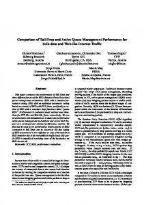
Network Topology UDP Sink
UDP
FTP
10 V a Mb p ri a s ble de
y ps ela Mb e d 1 0 ri a b l Va
lay Router
1.5 Mbps 10 ms delay
FTP Sink
Router
HTTP
HTTP Sink
HTTP
HTTP Sink
Figure 1: Dumbbell Topology The effects of different queueing algorithms on performance in a singlegateway scenario can be evaluated using a Dumbbell topology, see Figure 1. This configuration is well understood and widely implemented, and hence has been chosen for preliminary testing of the evaluation framework. Three parameters are used to define the Dumbbell topology: the bandwidth of the bottleneck link, its propagation delay and the range of per-flow round-trip times (RTTs). The latter is one of the parameters frequently overlooked in common simulation scenarios. The different RTTs between TCP flows impacts on the share of a router queue that a flow obtains [9]. Measurement studies have shown that RTTs found on the Internet can vary widely, with most RTTs in a range between 15 and 500 ms [10].
3.2
Traffic Mix
Creating a realistic model of Internet traffic necessitates the use of a large parameter set. These parameters are obtained from measurement studies [10, 11] of Internet traffic. A typical traffic mix used for the evaluation of router-queue management algorithms is that of long-lived FTP bulk-transfers. This mix is not representative of current Internet traffic: this is dominated by a high proportion of short-lived Web flows, or dragonflies, and a low number of long-lived transfers, or tortoises (which generate a large percentage of the traffic on the network) [11].
4
The effect of traffic that does not use end-to-end congestion control on network performance and throughput fairness should not be neglected [12]. The evaluation framework provides for the inclusion of such UDP traffic in any simulation scenario whilst the default traffic mix contains mainly Web-like traffic with background FTP and UDP flows.
4
Framework Implementation
The architecture of the framework is made up of two key components: a high-level interface for specifying simulation scenarios and experiments, and an engine for running several simulations in parallel.
4.1
High-level Interface
ns2 is the de-facto standard network simulator for Internet research. However, ns2 limits its higher-level functionality to a scripting interface. One of the requirements of the proposed evaluation framework is that it should be able to address research issues with a minimum of configuration or scripting complexity. In doing so it should address questions like: • What is the effect of increasing non-responsive UDP traffic on network performance and flow throughput fairness? • How well do Active Queue Management schemes perform under different Web traffic loads? • How sensitive to parameter settings is the performance of a given AQM scheme? Configuring and running the simulations that will address these issues using ns2 is a time-consuming process. It involves writing OTcl scripts for establishing the simulation scenarios in ns2, running numerous simulations and processing the output from ns2 to obtain results. Even though sample scripts are available for these tasks, running simulations, writing ns2 scripts and processing the output combine to make the process extremely time consuming. Moreover, ns2 does not provide any functionality to perform the output data analysis necessary to obtain credible simulation results. Poorly chosen network scenarios may further limit the usefulness of the results obtained and may even invalidate the results if the parameters chosen are unrealistic. Our framework uses ns2 as its “simulation engine” but provides a high level interface to it. The system has been initially targeted for AQM evaluation but can equally be used to address other network performance evaluation questions. It incorporates a Python API [13] offering two main functional groupings: 5
• An Experiment comprises a set of simulations that have a common set of fixed parameters and one variable parameter. The fixed parameters may be either user-specified or predefined default values. Experiments provide functionality for running the associated simulations and they calculate network performance metrics using the output data. For each simulation model a set of replications is run with independent streams of random numbers. From metrics values obtained in those replications estimates of mean values and their associated relative error level is reported. • The Report provides the main interface to the framework. It comprises a simplified way of specifying a set of experiments and obtaining results: The user specifies one or more parameter spaces to explore and the framework configures and runs the required ns2 simulations. The following sample script code illustrates how the framework may be used to obtain a report showing how a UDP traffic flow with increasing load affects network performance: report = Report() report.addPlotParam(’scenario.cbrBitrate’, range(0, 10.1)) report.addFixedParam(’stopTime’, 20) report.generate()
This five-line script will create and run eleven ns2 simulations for each supported AQM scheme. For each scheme the rate of offered UDP traffic will vary between 0 and 10 MB/s. Once all the simulations have finished, and their output parsed, a report is generated summarising the network performance. The framework supports numerous parameters, making it a powerful, high-level interface for carrying out simulation-based network performance experiments.
4.2
Parallel Simulation Engine
The evaluation framework may require several simulations to be performed for each set of results generated. It is common to find ns2 simulation scenarios requiring several minutes to finish using current workstation technology. Production of a report typically requires a large number of simulations to be performed. Hence, using a single workstation to generate reports is extremely time consuming. Sequential network simulators have been extended to run on parallel computers [14]. Our approach differs in that we obtain economies of scale by parallelising each experiment at the granularity of one simulation. Using the proposed framework typically involves running several simulations 6
Slave Listener 1 Renderer OTcl
XM Parallel Runner Controller Process
C L -R P
X ML -
Trace Parser Traces
NS Process
Slave Listener 2
RP C
Renderer OTcl
Trace Parser Traces
NS Process
Figure 2: Parallel Simulation Engine architecture
for each experiment. Substantial speed advantages may be obtained from distributing the load amongst a set of networked workstations. Individual simulations still run using a standard sequential ns2 simulator thus providing good scalability without the need for modification of the ns2 software. Figure 2 illustrates the architecture of the framework when using the parallel simulation engine with two “slave” hosts. The “slaves” execute the simulations and parse the output traces. The controller process communicates with the slaves using XML-RPC, a remote procedure call protocol based on HTTP and XML. The controller sends scenario parameters with the requests and the slaves reply with a summary of the results of the simulation. Once all the simulations have finished and their results have been collected, the framework calculates experiment-level network performance metrics.
5
Improving the framework credibility
As real networks increase in size and complexity, simulation is becoming the most important tool used for network performance evaluation. A recent survey by Pawlikowski et al. [15] found that stochastic discrete-event simulation (as implemented by ns2) was used in over half the studies published. While some have advocated better simulation models for Internet research [3], there seems to be little concern regarding the analysis and credibility of simulation results. It has been argued [15] that a credibility crisis exists due to the widespread lack of correct analysis of simulation output data. In this section the statistical techniques and procedures implemented
7
in the framework are described. These may be used to obtain meaningful results from simulation-based network performance studies.
5.1
Analysis of a single run
The framework should obtain steady-state values for the five metrics described in section 2, however for one single run of the simulation, two significant problems are encountered: • The estimation of the steady-state value is biased by use of an atypical initial state (i.e. empty queues and links). • Once the initial, transient, phase is over, it is necessary to determine how long the simulation run should be in order to obtain a good approximation to the steady-state mean. Possible methods for overcoming these problems are now discussed. 5.1.1
Initial Transient
The network model simulated is empty and idle at beginning of the simulation: all queues are empty and no traffic enters the network. These initial conditions usually introduce a bias as they are unrepresentative of the desired steady state. Different methods have been proposed to remove this warm-up period: Pawlikowski [16] presents 11 different methods which can be used to estimate the initial transient, while recent studies [17,18] present graphical, heuristic or statistical methods. To compute the length of the initial transient, a simple heuristic developed by White [19] is used. This method, called the Marginal Confidence Rule (MCR), selects the truncation point that minimises the width of the confidence interval about the truncate sample mean. If x1 , x2 , · · · , xN is the set of points measured during the simulated time, the optimal truncation point i ∈ [1, N ] is defined as: i = arg min
0≤i p × i (p has been set to 5 in the current version of the framework).
9
Metrics evolution for one replication 3
drop delay jitter utilization fairness
Normalized metric value
2.5
2
1.5
1
0.5
0
0
5
10
15
20
25
30
35
40
45
Time (s)
Figure 4: Convergence of the five metrics, with initial transient (the sample averages are normalised to their value at t = 40s).
5.2
Multiple Replications
Many network simulation studies construct a model, select performance metrics and conclude with a single simulation run to obtain results. The use of random values from particular distributions as simulator inputs means that the results obtained from a single simulation run are just the realisations of random variables [20]. Figure 5 illustrates how the point values obtained for an individual performance metric can vary considerably between statistically independent simulation runs. Hence, it is essential to use multiple independent replications of the same simulation model and proper statistical analysis of the resultant output data. This lowers the probability of obtaining erroneous results to an acceptable level and improves the credibility of the results obtained. When using multiple independent replications, the number of replications n can be established beforehand, using the fixed-sample-size procedure [20] method. When n is fixed, a point estimate and confidence interval for the mean µ = E(X) may be obtained (where X represents the values that the metric of interest takes in different replications). A point value X(n) can be used to estimate the mean µ and hence a
10
Fairness evolution for different replications 0.7
Replication 0 Replication 1 Replication 2 Replication 3
0.6
Fairness metric
0.5
0.4
0.3
0.2
0.1
0
0
5
10
15
20
25
30
35
40
45
Time (s)
Figure 5: Evolution of the Fairness metric over simulated time for different replications of a simulation
100(1 − α)% confidence interval for µ can be found: δ(n, α) = X(n) ± tn−1,1−α/2
s
S 2 (n) , n
(3)
where X(n) is the estimated mean, S 2 (n) is the sample variance and t(n,α) is the Student’s t distribution. The main disadvantage of the fixed-sample-size procedure is that it does not allow a predefined confidence interval half-length to be calculated. If a specific error or precision is desired for the estimated mean X(n) then the number of replications n must be calculated dynamically. The framework implements a method for dynamically deciding the number of replications required. The procedure used aims to be able to obtain an estimate mean X for µ with a relative error γ (0 < γ < 1) and a confidence of 100(1 − α)%, where α and γ are specified initially. The relative error is defined as γ = |X − µ|/|µ|, hence the percentage error in X is 100γ%. A sequential procedure for determining the number of replications n has been implemented in the framework. It starts with an initial number of replications n0 = 10, sets n = n0 and computes the estimated mean X(n) and the confidence interval half-length δ(n, α) given by (3). If δ(n, α)/|X(n)| ≤ γ0, 11
the relative error is below our desired threshold, so the current X is used as the point estimate for the mean metric value µ and no more replications are added. The current approximate 100(1 − α)% confidence interval is given by I(α, γ) = [X(n) − δ(n, α), X(n) + δ(n, α)]. (4) The number of replications n is incremented by 1 until a value of n is reached for which δ(n, α) is below the predefined threshold. Fairness evolution for different replications 0.7
Average (with confidence interval) Replication 0 Replication 1 Replication 2 Replication 3
0.6
Fairness metric
0.5
0.4
0.3
0.2
0.1
0
0
5
10
15
20
25
30
35
40
45
Time (s)
Figure 6: Fairness metric value over time without initial transient bias and estimated average with confidence interval. Figure 6 shows how the metric values evolve over the simulation run length once the bias introduced by the initial warm-up period has been eliminated. The estimated mean for the fairness metric with its associated confidence interval is also plotted on this graph. When comparing this graph with figure 5 it can be seen how the deletion of the initial transient improves the stability of the fairness values. The sequential procedure for determining the number of replications, when used in conjunction with the technique described in the previous section for eliminating initial transient bias, is known as the replication/deletion approach [20].
12
6
Study of the fairness of RED
The main purpose of the framework is to study the differences between AQM schemes. A full evaluation of these algorithms is outside the scope of this paper, rather we wish to demonstrate the use of the framework and its performance evaluation metrics. The RED algorithm [1] and its more recent variant, RED-PD [21] (RED with preferential dropping), are studied in this experiment. Drop-tail queue is also considered as it is the basic scheme implemented in current Internet routers. The algorithms considered are: • Drop-Tail: standard drop-tail queue. Packets are dropped only when buffer overflow occurs. • RED: the “current version” of RED, implemented in ns2 by its authors. It includes the gentle version (no discontinuities in the drop probability function), and improved parameter settings. • RED-PD: RED with preferential dropping [21], adds another layer to RED, detecting and penalising non responsive flows. Fairness with different UDP bitrates 1
RED-PD DropTail RED
Fairness Metric
0.8
0.6
0.4
0.2
0
0
5
10
15
20
UDB Bitrate (Mb/s)
Figure 7: Fairness Metric The experiment is based on a simple dumbbell scenario. The parameters being used are: 13
Drop rate with different UDP bitrates 0.7
RED-PD DropTail RED
0.6
Drop Metric
0.5
0.4
0.3
0.2
0.1
0
0
5
10
15
20
UDP Bitrate (Mb/s)
Figure 8: Drop Metric
• Bottleneck bandwidth: 10M b/s • Bottleneck delay: 10ms • RTT range: 20ms − 460ms This experiment examines the effect of the proportion of unresponsive traffic (UDP in this case) on performance. We focus here on the drop and fairness metrics Figures 7 and 8 show that the more recent improvement of RED — RED-PD — achieved its design objectives: RED with preferential dropping provides for more fairness, by the more aggressive dropping of incoming UDP packets. While RED is more aggressive than regular Drop-Tail, it exhibits comparable fairness. The high level framework interface allows for the easy setup of such experiments: the graphs produced in this section are taken from the report generated by a ten-line python script.
7
Future Work The framework may be extended in several ways.
14
The caching of results would yield significant performance enhancements: one simulation, of even the simplest dumbbell scenario, can take several minutes; while detailed experiments, involving higher bandwidth flows, can take several hours to run. Caching previous results in a database would enable the framework to be used for much more complex network simulation scenarios, thus increasing its utility as a research tool. More complex network topologies should also be supported. These may include the “reverse-dumbbell” topology with multiple congested gateways [22] and realistic Internet-like topologies such as power-laws [23]. It is planned to extend the framework so that it can interface with other network simulators such as GloMoSim or OPNET. This will allow the framework to seamlessly validate results across multiple simulators.
8
Conclusion
A framework for objective comparison and evaluation of AQM schemes is described. It incorporates five carefully chosen metrics characterising overall network performance. The highly configurable tool allows for easy exploration of the parameter space and provides consistent assessment of different AQM schemes making it an invaluable resource for AQM performance evaluation.
Acknowledgements This work has been supported by Enterprise Ireland Basic Research Grant, SC/2002/293.
References [1] S. Floyd and V. Jacobson, “Random early detection gateways for congestion avoidance,” IEEE/ACM Transactions on Networking, vol. 1, no. 4, pp. 397–413, Aug. 1993. [2] B. Braden et al., “Recommendations on queue management and congestion avoidance in the internet,” RFC 2309, Apr. 1998. [3] S. Floyd and E. Kohler, “Internet research needs better models,” in Proc. HotNets-I. ACM, Oct. 2002. [4] C. Zhu, O. Yang, J. Aweya, M. Ouellette, and D. Montuno, “A comparison of active queue management algorithms using the OPNET modeler,” IEEE Communications Magazine, vol. 40, no. 6, pp. 158– 167, June 2002.
15
[5] G. Iannaccone, C. Brandauer, T. Ziegler, C. Diot, S. Fdida, and M. May, “Comparison of tail drop and active queue management performance for bulk-data and web-like internet traffic,” in Proc. ISCC. IEEE, July 2001. [6] L. Breslau, D. Estrin, K. Fall, S. Floyd, J. Heidemann, A. Helmy, P. Huang, S. McCanne, K. Varadhan, Y. Xu, and H. Yu, “Advances in network simulation,” IEEE Computer, vol. 33, no. 5, pp. 59–67, May 2000. [7] G. Ewing, K. Pawlikowski, and D. McNickle, “Akaroa2: Exploiting network computing by distributing stochastic simulation,” in Proc. ESM’99. International Society for Computer Simulation, June 1999, pp. 175–181. [8] R. Jain, D. Chiu, and W. Hawe, “A quantitative measure of fairness and discrimination for resource allocation in shared computer systems,” Digital Equipment Corporation, Tech. Rep. DEC-TR-301, Sept. 1984. [9] S. Floyd, “Connections with multiple congested gateways in packetswitched networks - part 1: One-way traffic,” ACM Computer Communication Review, vol. 21, no. 5, pp. 30–47, Oct. 1991. [10] M. Allman, “A web server’s view of the transport layer,” ACM Computer Communication Review, vol. 30, no. 5, Oct. 2000. [11] N. Brownlee and K. Claffy, “Understanding Internet traffic streams: Dragonflies and tortoises,” IEEE Communications Magazine, vol. 40, no. 10, pp. 110–117, Oct. 2002. [12] S. Floyd and K. Fall, “Promoting the use of end-to-end congestion control in the Internet,” IEEE/ACM Transactions on Networking, vol. 7, no. 4, pp. 458–472, Aug. 1999. [13] G. van Rossum, “Python language website,” http://www.python.org. [14] H. Wu, R. M. Fujimoto, and G. Riley, “Experiences parallelizing a commercial network simulator,” in Winter Simulation Conference, Dec. 2001. [15] K. Pawlikowski, H.-D. Jeong, and J.-S. Lee, “On credibility of simulation studies of telecommunication networks,” IEEE Communications Magazine, vol. 40, no. 1, pp. 132–139, Jan. 2002. [16] K. Pawlikowski, “Steady-state simulation of queueing processes: A survey of problems and solutions,” ACM Computing Surveys, vol. 22, no. 2, pp. 123–169, June 1990. 16
[17] J. R. Linton and C. M. Harmonosky, “A comparison of selective initialization bias elimination methods,” in Winter Simulation Conference, vol. 2, Dec. 2002, pp. 1951–1957. [18] S. Robinson, “A statistical process control approach for estimating the warm-up period,” in Winter Simulation Conference, vol. 1, Dec. 2002, pp. 439–446. [19] J. K. Preston White, “An effective truncation heuristic for bias reduction in simulation output,” Simulation, vol. 69, no. 6, pp. 323–334, Dec. 1997. [20] A. M. Law and W. D. Kelton, Simulation Modeling and Analysis, 3rd ed. McGraw Hill, 2000. [21] R. Mahajan and S. Floyd, “Controlling high bandwidth flows at the congested router,” AT&T Center for Internet Research at ICSI (ACIRI), Tech. Rep. TR-01-001, Apr. 2001. [22] K. Anagnostakis, M. Greenwald, and R. Ryger, “On the sensitivity of network simulation to topology,” in Proc. MASCOTS’02. IEEE, Oct. 2002, pp. 117–126. [23] M. Faloutsos, P. Faloutsos, and C. Faloutsos, “On power-law relationships of the internet topology,” in SIGCOMM’99. ACM, Sept. 1999, pp. 251–262.
17
A
Appendix In this appendix, we defined the metrics for a single simulation run.
A.1
Notation
The total simulation time is denoted by τ and the network capacity by C. During τ there are F active flows indexed by i ∈ [1, F ]. For flow i, we define the following variables: • Si , the total size of the data received • Si0 , the total size of the data sent • Ni , the number of packets received • µi , the average delay, weighted by packet size • νi , the weighted variance of the delay
A.2
Metric Definitions
The five metrics used for network performance evaluation are: A.2.1
Utilisation metric PF
i=1 Si
Cτ
A.2.2
Fairness metric ´2 F S i i=1 PF 2 i=1 Si
³P
F
A.2.3
Delay metric
(7)
PF
(8)
PF
i=1 Si
Jitter metric
(6)
PF
i=1 Si µi
A.2.4
(5)
Si νi i=1 µi PF i=1 Si
18
A.2.5
Drop metric PF
Si 0 i=1 Si
A.3
1 − PFi=1
(9)
Computation of the Metrics
Consider flow i, i ∈ [1, F ]. For all received packet p, p ∈ [1, Ni ], we may find the delay experienced by the packet di,p and its size si,p by analysis of the output trace file. To simplify the calculations of the delay and jitter metrics, dummy variables Ai and Bi are computed: Ai =
Ni X
si,p
p=1
and Bi =
Ni X
si,p di,p
p=1
Ai , Bi , Ni , Si , and Si0 , are computed incrementally while parsing the trace file generated by ns2. The utilisation, fairness and drop metrics may be easily computed using Si and Si0 in the given formulae (resp. in equations 5, 6, and 9). While from equation 7, it is noted that the delay metric depends on: S i µi = B i
(10)
Finally, we need to compute Sµi νi i in order to evaluate the jitter metric using equation 8. The weighted delay variance νi is given by: Ni νi = × Ni − 1
Hence, Si νi µi
= =
Ni × Ni − 1
P Ni
p=1 si,p (di,p
P Ni
Si
p=1 si,p (di,p
P
Ni × Ni − 1
− µi )2
.
− µ i )2
µi Ni 2 p=1 si,p di,p µi
+ µi
Ni X
p=1
si,p − 2
Ni X
p=1
si,p di,p
and using the predefined variables Ai and Bi this may be simplified to: Si νi µi
=
Ni Ni − 1 19
µ
Ai Si − Bi . Bi 
(11)