A Framework for Evolutionary Optimization With ... - CiteSeerX

IEEE TRANSACTIONS ON EVOLUTIONARY COMPUTATION, VOL. 6, NO. 5, p p . 4 8 1 - 4 9 4 , OCTOBER 2002

A Framework for Evolutionary Optimization With Approximate Fitness Functions Yaochu Jin, Senior Member, IEEE, Markus Olhofer, and Bernhard Sendhoff, Member, IEEE

Abstract—It is not unusual that an approximate model is needed for fitness evaluation in evolutionary computation. In this case, the convergence properties of the evolutionary algorithm are unclear due to the approximation error of the model. In this paper, extensive empirical studies are carried out to investigate the convergence properties of an evolution strategy using an approximate fitness function on two benchmark problems. It is found that incorrect convergence will occur if the approximate model has false optima. To address this problem, individual- and generation-based evolution control are introduced and the resulting effects on the convergence properties are presented. A framework for managing approximate models in generation-based evolution control is proposed. This framework is well suited for parallel evolutionary optimization, which is able to guarantee the correct convergence of the evolutionary algorithm, as well as to reduce the computation cost as much as possible. Control of the evolution and updating of the approximate models are based on the estimated fidelity of the approximate model. Numerical results are presented for three test problems and for a aerodynamic design example. Index Terms—Approximate fluctuations, evolutionary computation, fitness functions, optimization.

I. INTRODUCTION

E

VOLUTIONARY algorithms are known to be robust optimizers that are well suited for discontinuous and multimodal objective functions [1], [2]. For this reason, evolutionary algorithms have been applied successfully to a variety of complicated real-world applications, such as aerodynamic design optimization [3], [4], circuit design [5], routing [6], and scheduling [7]. One essential difficulty in employing evolutionary algorithms in such applications is the huge time consumption due to the high complexity of performance analyses for fitness evaluation and the large number of evaluations needed in the evolutionary optimization. To address this problem, approximate models that are computationally efficient are often used to reduce the computation time. Another important area of evolutionary computation in which approximate models can play an important role is interactive evolutionary computation [8]. In interactive evolutionary computation, there is no explicit fitness function, and the fitness evaluation is performed directly by a human expert. Interactive evolutionary computation has found a wide range of applications, such as graphics and art design [9], music generation [10], and layout design [11]. As pointed out in [8], the main difficulty in interactive evolution is how to relieve the fatigue of the Manuscript received November 8, 2000; revised October 1, 2001. The authors are with the Future Technology Research, Honda R&D Europe, 63073 Offenbach/Main, Germany (e-mail: [email protected]). Publisher Item Identifier 10.1109/TEVC.2002.800884.

involved human. One solution to this problem is the introduction of an approximate model that can model the process of the human’s evaluation. In [12], a neural network has been used to model the behavior of the human to reduce human fatigue. In addition, approximate models can also be used to smooth the rough fitness functions and thus prevent the evolutionary algorithm from stagnating in a local optimum [13], [14]. In these papers, the performance of evolutionary algorithms has been improved for a number of multimodal test functions by combining local search techniques with approximate models. Several methods have been developed for constructing approximate models. One widely used method in design engineering is the response surface methodology, which uses low-order polynomials and the least square estimation [15]. A more statistically sound method is the Kriging model, which is also known as the design and analysis of computer experiments (DACE) model [16]. In this method, a global polynomial approximation is combined with a local Gaussian process and the maximum likelihood measure is used for parameter estimation. Artificial neural networks, including multilayer perceptrons (MLP) and radial basis function networks (RBFN), have also been employed to build approximate models for evolutionary optimization. A comprehensive review of different approximation concepts is provided in [17] and a comparison of the different techniques can be found in [18]–[20]. However, it is generally difficult to get a model with sufficient approximation accuracy, mainly due to the lack of data and the high dimensionality of many real-world problems. Therefore, approximate models often have large approximation errors and can even introduce false optima. In this case, the evolutionary algorithm with approximate models for fitness evaluation may converge incorrectly [21] and measures must be taken to guarantee that the solution discovered is optimal or near-optimal. In optimization, the use and manipulation of approximate models is usually referred to as model management. In [22], a framework for managing approximate models was proposed based on the classical trust-region methods [23], [24]. An extension of this work was reported in [25]. One main feature of the framework for managing approximate models is the strong interplay between the optimization and the fidelity of the approximate model based on the trust-region method, which ensures that the search process converges to a reasonable solution of the original problem. Managing approximate models in optimization based on evolutionary algorithms has not received much attention, although the idea of using different levels of approximation in evolutionary algorithms can be traced back to 1960s [26]. Most methods for using an approximate model for fitness

1089-778X/02$17.00 © 2002 IEEE

1

2

IEEE TRANSACTIONS ON EVOLUTIONARY COMPUTATION, VOL. 6, NO. 5, OCTOBER 2002

evaluations assume that the approximate model is correct and the evolutionary algorithm will converge to a global or near-optimal solution. Under this assumption, the most straightforward approach is to use an approximate model or a reduced model during the entire evolutionary optimization process [27], [28]. These methods can only be successful when the approximate model is globally correct. In [29], a heuristic convergence criterion is used to determine when the approximate model must be updated. The basic idea is that the convergence of the search process should be stable, which means that the change of the best solution should not be larger than a user-defined value. An assumption is that the first sets of data points are at least weakly correlated with the global optimum of the original problem, which is not necessarily true for high-dimensional systems. In another approach [30], the original fitness function is employed in every generations. That is to say, the approximate model th generation, the is used for generations and in the original fitness function is used and the data obtained from this generation are used to update the approximate model. As shown in [21], the evolution process may become very unstable if there is a large discrepancy between the approximate model and the original fitness function. In [31], a neural network is trained with some initial samples to approximate the NK (AU: PLS. DEFINE NK) model [32]. During evolution, the fittest individual in the current population is evaluated on the original fitness function once in every 50 generations. This individual then replaces the one with the lowest fitness in the training set, and the neural network is retrained. It is found that the evolutionary algorithm is misled by the neural network model when the complexity of the original fitness landscape is high. A similar method has been used in [33], where the best individual is reevaluated using the original fitness function in every generation. An approach to coupling approximate models with evolutionary algorithms is proposed in [34] in an attempt to balance the concern of optimization with that of the design of experiments. The main idea is to maintain the diversity of the individuals and to select those data points that are not redundant for model updating (on-line learning). In this method, the decision of when to carry out the online learning of the approximate model is simply based on a prescribed generation delay. The common weakness in the above methods is that neither the convergence of the evolutionary algorithm with approximate fitness functions (correct convergence is assumed) nor the issue of model management is addressed. In this paper, the convergence property of the evolutionary algorithms with approximate fitness evaluation is first investigated on two benchmark problems. We show that incorrect convergence occurs when the approximate fitness function has false optima [21]. A large network error that is uniform over the whole search space does not pose a problem. However, if the error significantly depends on the local topology, false minima can occur and the optimization process can be misled by the neural network model. To improve the convergence of the evolutionary algorithm, we introduce the concept of evolution control, in which the evolution proceeds based on fitness evaluations using not only the approximate fitness model, but also the original fitness function. There are two possibilities to combine

the original fitness function with the approximate fitness function. In the first approach, a certain number of individuals within a generation are evaluated with the original fitness function. Such individuals are called controlled individuals. The second approach is to introduce controlled generations, which means generations, generations are conthat in every trolled. In a controlled generation, all individuals are evaluated with the original fitness function. The most important question is how many individuals or how many generations should be controlled to guarantee the correct convergence of an evolutionary algorithm when false optima are present in the approximate fitness function. To answer this question, simulations have been carried out on the Ackley function [35] and the Rosenbrock function [36], which have been studied widely in the field of evolutionary computation. Based on these empirical studies, a framework for model management in generation-based evolution control is proposed. Generally, generation-based evolution control is more suitable when the evaluation of the fitness function is implemented in parallel. The main idea is that the frequency at which the original function is called and the approximate model is updated should be determined by the local fidelity of the approximate model. By local fidelity, we mean the fidelity of the model for the region where the current population is located. The lower the model fidelity, the more frequently the original function should be called and the approximate model should be updated. Since it is virtually impossible to build a globally correct approximate model for problems with a large dimensionality of the design space, a local model is of more practical importance. With this strategy, the computational cost can be reduced as much as possible while the correct convergence of the evolutionary algorithm can still be guaranteed. An evolution strategy with covariance matrix adaptation (CMA) [37] is adopted in this work because the algorithm converges very quickly and because it allows us to take advantage of the self-adaptation of the covariance matrix in online training of the neural network model. The basic idea is that the new data points that lie along the direction in which the evolutionary algorithm proceeds should be given larger weight in online learning. Interestingly, the rough information on the directions to search is contained in the covariance matrix. Results from the benchmark problems show that better performance can be achieved when the covariance matrix is used to weight the new samples in online learning. The remainder of the paper is organized as follows. Section II presents the evolution strategy along with an explanation of the covariance matrix adaptation. The parallel implementation of the evolutionary algorithm is also described briefly. In Section III, the convergence of the evolutionary algorithm with approximate fitness functions is investigated empirically on the Ackley function and the Rosenbrock function. Based on these results, two approaches to evolution control are suggested for improving the convergence of the evolutionary algorithm with approximate fitness functions. A framework for evolutionary optimization with approximate fitness functions is proposed in Section IV, which includes the control strategy, the determination of the frequency for evolution control and online learning, as well as the weighted learning algorithm on the basis of the

JIN et al.: FRAMEWORK FOR EVOLUTIONARY OPTIMIZATION WITH APPROXIMATE FITNESS FUNCTIONS

covariance matrix. This framework is employed on three benchmark problems and a real-world application. In the application, neural network models are used to approximate the computationally very intensive computational fluid dynamics (CFD) analyses. With the help of the proposed model management framework, the performance of the evolutionary optimization has been improved significantly with the same number of CFD evaluations. The final optimal design of the blade is verified by CFD simulations. II. EVOLUTION STRATEGY AND ITS PARALLEL IMPLEMENTATION

3

The derandomized CMA [37] differs from the standard ES mainly in three respects. 1) In order to reduce the stochastic influence on the self-adaptation, only one stochastic source is used for the adaptation of both objective and strategy parameters. In the derandomized approach [41], the actual step size in the objective parameter space is used to adapt the strategy parameter. Therefore, the self-adaptation of the strategy parameters depends more directly on the local topology of the search space. In the case of the adaptation of one strategy parameter, this can be written as: (5)

A. Evolution Strategy With Covariance Matrix Adaptation The canonical evolution strategy (ES) operates on an -di. The main operator in ES is the mumensional vector tation operator. However, unlike in the canonical genetic algorithm (GA) [1], but similar to evolutionary programming (EP) [38], the mutation operator obtains a direction during search due to the self-adaptation of the strategy parameters. The combination of the genotypes from different parents, carried out by the recombination operator in ES or the crossover operator in GA, usually plays a less significant role or is omitted completely as in this study.1 The ES is typically combined with a determin-ES, or istic selection method, either with elitism, i.e., -ES. At the same time, the combinawithout elitism, i.e., tion with other selection methods, e.g., EP tournament selection, has been reported to be successful [39]. In this work, we applied -ES, thus new individuals were only selected from the the offspring. The canonical ES can be described as follows [40]: (1) (2) (3) and where is the parameter vector to be optimized and are the strategy parameters. The values for and are usually fixed to (4) The , , and are normally distributed random numbers and a random number vector, respectively, which characterize the mutation exercised on the strategy and the objective parameare also called step sizes and are subject to selfters. The adaptation, as shown in (2). Since they define the variances of the normal probability distribution (3) for the mutation in (1), they stochastically define a direction and a step size of the search process in the -dimensional space. However, arbitrary directions can only be represented by correlated mutations, i.e., the covariance matrix of the normal distribution should have nonzero off-diagonal elements. Such correlated mutations are realized by the covariance matrix adaptation (CMA) algorithm that is outlined in the remainder of this section. 1In the design optimization experiments described in Section V, the recombination operator turned out to not be beneficial.

(6) where parameter is used to regulate the adaptation. Therefore, in the derandomized approach, the actual step size in the objective parameter space is used to adapt the strategy parameter. This results in the following simple, but successful, effect. If the mutation was larger , then the strategy than expected parameter is increased. This ensures that if this larger mutation was successful, i.e., the individual was selected, then in the next generation such a larger mutation is was increased. The likely to occur again, because . same argumentation holds if 2) The second aspect is the introduction of the cumulative step-size adaptation. Whereas the standard evolution strategy extracts the necessary information for the adaptation of the strategy parameters from the population (ensemble approach), the cumulative step-size adaptation relies on information collected during successive generations (time averaged approach). This leads to a reduction of the necessary population size. The cumulation of steps was termed evolution path by Ostermeier and Hansen [37] and is expressed formally as (7) The factor determines the length of the evolution path, is needed for normalizaand the factor tion, which can be seen by calculating the variance of in the limit . 3) In the CMA algorithm, the full covariance matrix of the probability density function

(8) is adapted for the mutation of the objective parameter vector. The following description of the CMA algorithm follows the one given in [42] details of the implementation can be found in [43]. If the matrix satisfies and , then . The adaptation of the objective vector is given by (9)

4


where is the overall step size. The adaptation of the covariance matrix is implemented in two steps using the cuand ) mulative step-size approach ( determine the influence of the past during cumulative adaptation)

(10) (11) The next step is to determine the matrix from . Since is not sufficient to derive , we choose the as column vectors of . The reason eigenvectors of is that in the last step the overall step-size has to be adapted. In order to perform this adaptation, we have to know the expected length of the cumulative vector . Therefore, the variation vector, which depends on , distributed. This can be realized by should be normalizing the column vectors of by the square root of the corresponding eigenvalues, which yields the matrix , if the column vectors of are the eigenvectors of . Finally, the adaptation of and is given by

(12) (13) equals with normalized columns in order for to be distributed. denotes the exdistribution, which is the distribution pectation of the distributed random vector. of the length of an The CMA algorithm relies on several external parameters which have to be fixed manually. Since it is beyond the scope of this paper to introduce the details of the CMA algorithm, please refer to the literature for a discussion of appropriate choices [42], [43], [37].

where

B. Parallel Implementation of the Evolutionary Algorithm The basic motivation to implement an evolutionary algorithm in parallel is to reduce the processing time needed to reach an acceptable solution. This is badly needed when the evaluation of the fitness takes a large amount of time. There are several approaches to parallelization [44], and the one we adopt here is the global parallelization. In this approach, there is one population and the evaluation of the individuals is performed in parallel. For design problems, the evaluation of the individuals usually takes up the overwhelming part of the total time consumption; therefore, a sublinear speedup can be achieved if global parallelization approach is used. The hardware for the implementation of parallel evolutionary algorithms can be very different. In our case, a network of computers with multiprocessors is used. The implementation of the parallelization is realized with the parallel virtual machines library [45].

(a)

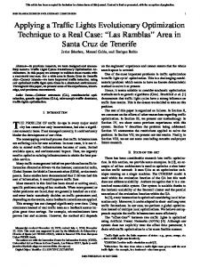
(b) Fig. 1. (a) 2-D Ackley function and (b) neural network approximation of the function with samples from one run of evolution.

III. EMPIRICAL CONVERGENCE STUDIES AND EVOLUTION CONTROL A. Convergence of the Evolution Strategy With Neural Networks for Fitness Evaluations In this section, we empirically investigate the convergence properties of the evolution strategy when a trained MLP neural network is used for fitness evaluations.2 The investigation is carried out on two benchmark problems: the Ackley function and the Rosenbrock function. The Ackley function is a continuous, multimodal test function, which has the following form:

(14) where is the natural base and is the dimension of the function. The two-dimensional (2-D) Ackley function is illustrated in Fig. 1(a). A neural network is trained to approximate the 2-D Ackley function. In the simulation, 600 training data are collected from one run of evolution with the Ackley function as the objective function. This is to simulate the situation that training 2In

this paper, the evolutionary algorithm is used for minimization problems.


data are only available from earlier optimization attempts in real-world applications. The MLP network used has one hidden layer with 20 nodes. The root-mean squared (rms) error on the training data is 0.20 and the input–output mapping is shown in Fig. 1(b). It can be seen that a false minimum exists at the right . This can be asside of the surface, near cribed to the poor distribution of the training samples. We deliberately use such samples to simulate the situation frequently encountered in practice, i.e., sparse and poorly distributed training data. Recall that for the problems we are discussing, data collection is expensive. If we run the evolutionary algorithm with this neural network model, the algorithm converges to the false minimum, which is an expected result. To show that the problem we identified above is a general one, simulations are also conducted with the Rosenbrock function

5

(a)

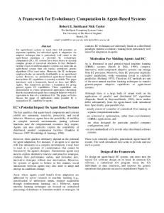
(15) where is the dimension of the function. For this function, the evolutionary algorithm is expected to easily find a near minimum. However, since the fitness function spans from thousands to zero, the mapping is more difficult to learn and in turn it will be more difficult to obtain the correct global minimum. The simulations are conducted for the 2-D case, the function is shown in Fig. 2(a). We generate 150 samples from one run of evolution with the 2-D Rosenbrock function, which is much smoother compared to the Ackley function. The mapping learned by the neural network is given in Fig. 2(b). Comparing it with the true 2-D Rosenbrock function, it is seen that the left ramp of the 2-D Rosenbrock function becomes almost flat due to the poor distribution of the training data. No doubt, evolution with this neural network model is vulnerable to serious errors because the global minimum of this approximate model lies in the area where the true value is very large. Therefore, an evolutionary optimization based on such an approximate model will converge to the false minimum. B. Adding Random Samples One straightforward idea of dealing with the problem is to add some randomly generated samples for neural network training, first without considering the cost of data generation. In the simulation, 150 random samples are added to the original training data, both for the 2-D Ackley function and the 2-D Rosenbrock function. It is found that the neural networks are able to learn the main features of the functions and no false minima are present. This is confirmed by running the evolutionary algorithm with the neural network model as the fitness function, in which a near-optimum is found for both functions. Unfortunately, adding random samples does not work for high-dimensional systems. To illustrate this, simulations are conducted with the 12-dimensional (12-D) Ackley function and the 12-D Rosenbrock function. In both cases, 450 randomly generated samples are added to 1000 training data. We only add 450 random samples just because in many real applications, it is impossible to collect sufficient data. Despite the neural networks having achieved a lower approximation error on

(b) Fig. 2. (a) 2-D Rosenbrock function and (b) the neural network approximation of the 2-D Rosenbrock function with training data from one run of evolution.

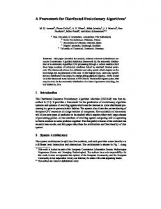
the training data, incorrect convergence has occurred for both functions, which is shown in Fig. 3(a) and (b). C. Improvement of Convergence With Controlled Evolution In Section III-C, it was shown that using additional training samples is not effective for dealing with the problem of “incorrect” convergence of evolutionary algorithms with neural network models. Therefore, we introduce the concept of evolution control. Two methods are proposed. 1) Controlled Individuals: In this approach, part of the indiin the population ( in total) are chosen and viduals evaluated with the original fitness function. If the controlled individuals are chosen randomly, we call it the random strategy. If we choose the best individuals as the controlled individuals, we call it the best strategy. 2) Controlled Generations: In this approach, the whole population of generations will be evaluated with the original . fitness function in every generations, where Furthermore, when controlled individuals or controlled generations are introduced, new training data are available. Therefore, online learning of the neural network will be applied to improve the approximation quality of the network model in the region of optimization and in turn to improve the convergence of the evolutionary algorithm. We first investigate the individual-based methods for the 12-D Ackley function. To determine the number of individ-

6


(a)

(a)

(b) Fig. 4. Convergence of ES with controlled individuals: (a) random strategy and (b) best strategy. Dashed line: the best fitness reported by the evolutionary algorithm. Solid line: the verified fitness value.

(b) Fig. 3. Incorrect convergence of the evolutionary algorithm for: (a) 12-D Ackley function and (b) 12-D Rosenbrock function. Solid line: fitness value calculated using the neural network model. Dashed line: true fitness.

uals that need to be evaluated using the original fitness function to guarantee correct convergence, different values of are tested for both the random strategy and -ES. The best fitness the best strategy for a found by the ES with the random strategy for different is shown in Fig. 4(a) by the dashed line. Since both the neural network model and the original fitness function have been used for the fitness evaluation, the reported best fitness is verified using the original fitness function when the evolution process is completed. The verified best fitness is denoted by the solid line. All the results are averaged over ten runs and both the mean value and the standard deviation are shown in the figures. It can be seen that for the random strategy, correct convergence . The of the evolutionary algorithm is not achieved until result using the best strategy is better, as shown in Fig. 4(b). When four out of 12 individuals are evaluated with the original fitness function, the average value of the reported best fitness

lies within the error bounds of the true fitness value. When is larger than 7, the reported average best fitness agrees with the average true fitness value. The results from the generation-based method are shown in Fig. 5(a), which are also averaged over ten different runs. In the figure, the coordinate denotes the number of generations in which all the individuals are evaluated with the original fitness function in every 12 generations. For example, if equals 8, then in every 12 generations, the original fitness function will be used in eight of the 12 generations. In this way, we are able to compare the results obtained in the generation-based method with the results in the individual-based strategies, because in both cases, the same entails the same computational overhead. Notice that it is determined randomly in which generations out of 12 generations the original function is used. It can be seen that a correct convergence has been achieved when is larger than 6. Once the original fitness function is used in evolution, new data are available and online learning can be implemented. In the following, we investigate in which way the algorithm can benefit, if these newly available data are used to train the neural network online. The result from generation-based evolution control with online learning is given in Fig. 5(b). The reported best fitness value is much closer to the true value compared to the case


(a)

(b) Fig. 5. Convergence of ES. Generation-based control (a) without and (b) with online learning. Dashed line: the best fitness reported by the evolutionary algorithm. Solid line: the verified fitness value.

where no online learning is implemented. Already for , the average values lie within the respective error bounds of the other values. When about 50% of the whole population is evaluated with the original fitness function, a good near-optimal or optimal solution has been found. Similar results have been obtained for the 12-D Rosenbrock function using the individual-based evolution control. Fig. 6(a) shows the convergence of the evolutionary algorithm for different values, where the best strategy is applied. It is seen that , the algorithm converges to the correct fitness value. when When online learning is introduced, the convergence properties are improved considerably and the resulting solution is near op[see Fig. 6(b)]. In both cases, the results are timal when based on an average of ten runs. In the following, we briefly compare the convergence properties using the 12-D Ackley function for the different individual-based strategies. In Fig. 7, the solid line denotes the percentage of correct convergence when the random strategy is adopted, while the dashed and dotted lines represent the percentage of correct convergence when the best strategy is used and when online learning is applied. It is shown that the best strategy works much better than the random strategy and online learning can further improve the convergence properties.

7

(a)

(b) Fig. 6. Convergence of ES for the Rosenbrock function (a) with best strategy and (b) with best strategy and online learning. Dashed line: the best fitness reported by the evolutionary algorithm. Solid line: the verified fitness value.

Fig. 7. Percentage of correct convergence. Solid line: random strategy. Dashed line: best strategy. Dotted-dashed line: best strategy with online learning.

IV. A FRAMEWORK FOR MANAGING APPROXIMATE MODELS In this section, a framework for managing approximate models in evolutionary optimization will be suggested. Taking into account the fact that parallel evolutionary algorithms are often used for design optimization, the generation-based evolution control strategy is used in this framework.

8


A. Generation-Based Evolution Control As suggested in Section III, generation-based evolution control is one of the approaches to guarantee the correct convergence of an evolutionary algorithm when the approximate fitness model has false minima. The idea behind the generationbased evolution control is that in every generations, there are generations that will be controlled, where . It is shown in to ensure correct conthe last section that should be about vergence when false global minima are present in the approxis imate model. However, an adaptive control frequency desirable so that the use of the time-consuming original fitness function can be reduced as much as possible without affecting the correct convergence of the algorithm.

It is intuitive that the higher the fidelity of the approximate model, the more often the fitness evaluation can be made using the model and the smaller can be. However, it is very difficult to estimate the global fidelity of the approximate model. Thus, a local estimation of the model fidelity has to be used. This is feasible because the ES generally proceeds with small steps, i.e., with the normal distribution, small mutations are most likely. Therefore, we can use the current model error to estimate the local fidelity of the approximate model and then to determine the frequency at which the original fitness function is used and the approximate model is updated. In our case, the frequency . When is fixed, the frequency is solely is denoted by determined by . To get a proper , heuristic fuzzy rules can be derived as follows: then

where is the true fitness value and is the fitness calculated using a feedforward neural network model (18) is the number of hidden nodes, is the number of where and are the weights in the input layer and output inputs, is the logistic function layer, respectively, and (19)

B. Determination of Control Frequency

If the model error is Large

Fig. 8. Algorithm for evolutionary optimization with approximate models. (AUTHOR: PLS. SUPPLY FIGURE)

is Large

Since the rule system has only one input variable, the number of fuzzy rules in total equals the number of fuzzy subsets used for the input variable. For simplicity, the input–output mapping of the fuzzy system can be approximately expressed by (16) denotes the largest integer that is smaller than where is the maximal , and usually equals 1 so that the information on the model fidelity is always available. is the allowed maximal model error and is the current model error estimation, and denotes the th cycle of generations. For convenience, we call every generations a cycle. The estimation of the current model error is carried out before the next cycle begins. Suppose all the new data in the last generations are valid (in aerodynamic design, some design may result in unstable fluid dynamics and therefore the data may be data invalid) and the population size is , then there will be in total. Thus, the model error is estimated as follows:

(17)

The framework for evolutionary optimization with approximate models is shown in Fig. 8. Note that this framework of controlling and adapting the model and the model frequency is independent of the choice of the evolutionary algorithm and the type of the model. The only restriction is that the model can be adjusted online. Recall that the fidelity of the model is estimated locally based on the error information from the last cycle. Therefore, should not be too large. C. Weighted Online Learning Using the Covariance Matrix An important issue in online learning is how to select new samples for network training to improve the model quality as much as possible. A simple way is to use all the new samples, or a certain number of the most recent data, if the neural network can learn all the data well. Unfortunately, in online learning, only a limited number of iterations of training are allowed to reduce the computation time. Various methods for data selection in neural network training are available, and are usually termed as active learning [46]–[49]. However, each of these methods relies on sufficient data in order to employ methods from statistics. In the problem outlined in this paper, data are sparse and their collection is computationally expensive. At the same time, information about the topology of the search space and, even more importantly, about the direction of the search process is contained in the covariance matrix, which is adapted during the evolutionary process (see Section II). To exploit this information, we suggest using the shape of the normal distribution [(8)] to weight the newly generated samples. In this way, the neural network will put more emphasis on the data points that the ES will most probably visit in the next generation. Covariance-based weighted online learning is shown schematically for a 2-D search space in Fig. 9. The topology is represented by lines of equal fitness. The normal distribution is shown as the gray ellipsoid, the grayscale corresponds to the decreasing probability. The dashed lines highlight the search “corridor.” The direction and the relative scale of the main axes are given by the covariance matrix. The lower two triangles denote data samples with large weights, and the top triangle denotes a data sample with a small weight. The samples marked with dots outside the search “corridor” will not be learned because the


9

on the Ackley function, the Rosenbrock function, the Rastrigin function, and an aerodynamic design example. A. The 20-Dimensional (20-D) Ackley function. A (2, 12) evolution strategy with covariance Ackley Function

Fig. 9. Schematic outline of the covariance-based weighted online learning. Explanation provided in the main text.

weight will be smaller than a given threshold (see below). The sample denoted by a dot at the bottom of the figure will receive a relatively large weight albeit it is not in the direction toward the main optimum. This is due to the symmetry of the normal distribution. Suppose there are new samples in total, then the cost function for weighted learning is given by (20) is the weight for sample , which is calculated from where the covariance matrix (21) is the input–output pair to be learned, is a where point in the current parent population to be referenced, usually the one represented by the best individual in the current population, is the covariance matrix defined in (8) in Section II. If the parameter vector is close to the origin (zero), Eq. (21) can be approximated by (22) Before applying the weights to neural network learning, they need to be normalized (23) is the maximal weight among . where In this way, the neural network is able to learn the most important samples, and those with a weight smaller than a given threshold are discarded in learning. V. NUMERICAL EXAMPLES To verify the feasibility of the proposed approach to managing approximate models, numerical studies are carried out

The first experimental study is conducted on the 20-D Ackley function. A (2, 12) evolution strategy with covariance matrix adaptation is adopted. In the simulation, is set to 6, is set to 1. The maximal number of generations is 300. to 4 and The results, including the best fitness and the number of calls of the original fitness function, are listed in Table I. The average best fitness over ten runs is 0.98 with a standard deviation of 0.41. The average number of generations that needs to be controlled within an evolution control cycle is 2.33. It is seen that the frequency at which the original fitness function needs to be called to guarantee correct convergence is much lower than 50% as suggested in Section III through the proper estimation of the model fidelity. To show that we can benefit from the introduction of the approximate model, we implement the optimization without using the approximate model but with the same number of evaluations of the original function. In the ten runs, the average number of calls of the original fitness function is 1440, which corresponds to 122 generations for a population size of 12. Therefore, we conduct ten runs of the evolution with a maximal number of generations of 122, for which the results are presented in Table II. The average best fitness resulting from the ten runs is 2.33. Comparing it with the average fitness using the approximate model with approximately the same computational overhead, the benefit of using the model becomes evident. Note, that we assume that the computational cost of the approximate model is negligible compared to that of the original fitness function. In the above simulation, all new data are used for network training. In the following, we introduce the weighted learning based on the covariance matrix. In the simulation, it is found that the use of weighted learning should be introduced after the evolution process becomes relatively stable. This may be due to the fact that at the beginning of the evolution, the information obtained by the evolutionary algorithm is still inaccurate; the covariance matrix is not adapted yet to the topology of the search space. The results are presented in Table III. Notice that in ten runs, the best fitness on average is further improved, while the average number of calls of the original function remains approximately the same (fewer than 4 generations in total). The standard deviation is 0.32 for the best fitness and 77.8 for the number of calls. B. The 20-D Rosenbrock Function Simulations are also carried out on the 20-D Rosenbrock function. As for the Ackley function, simulations are carried out for three different cases, namely, evolution using both the approximate model and the original model (Table IV, evolution using the original model only (Table V), and evolution with a combination of the approximate model and the original model with weighted learning (Table VI). When the generation-based evolution control is used, the average best fitness is 35.5 with a standard deviation of 10.5 over ten runs. Over ten runs, 865 calls of the original function are

10


TABLE I GENERATION-BASED EVOLUTION CONTROL

TABLE II EVOLUTION WITH THE ORIGINAL FUNCTION ONLY

TABLE III GENERATION-BASED EVOLUTION CONTROL WITH WEIGHTED ONLINE LEARNING

TABLE IV GENERATION-BASED EVOLUTION CONTROL

TABLE V EVOLUTION WITH THE ORIGINAL FUNCTION ONLY

TABLE VI GENERATION-BASED CONTROL WITH WEIGHTED ONLINE LEARNING

made on average in 200 generations. Since 865 calls equal approximately 73 generations with a population size of 12, we then run the evolution for 73 generations with the original function only. The average best fitness is 207.3 with a standard deviation of 204.7. Therefore, a much better result has been achieved with the help of the approximate model. Finally, we introduce the weighted online learning. The average best fitness is 28.1 with a standard deviation of 12.3, again better than the results without weighted online learning. We notice that additional 83 calls of the original function are needed in this case, which corresponds to seven generations. Therefore, we conduct another ten runs with 100 generations using the original fitness function only and the average best fitness is 87.4. C. The 10-D Rastrigin’s Function The -dimensional Rastrigin function is a multimodal test function, which has been studied in both [30] and [14]: (24)

Similar to [30], all variables are restricted to and the number of fitness evaluations is limited to 1000 in optimization. When only the original fitness function is used, the average best fitness is 12.7 with a standard deviation of 3.89 over ten runs. Then, an approximate model is used together with the original fitness function in optimization. The average best fitness is 1.1 with a standard deviation of 1.96. D. Aerodynamic Design Optimization One of the main difficulties in aerodynamic design optimization is the tremendous time consumption in quality evaluation. Generally, a 2-D or three-dimensional (3-D) Navier–Stokes solver with a turbulence model is used for computing the fluid dynamics, which usually takes hours of CPU time to get a solution. The objective of the optimization in our study is to maximize the efficiency of a turbine blade and to minimize the bias of the outflow angle from a prescribed value. The maximization of efficiency is realized by the minimization of the pressure loss. In addition, mechanical constraints must be satisfied concerning stability and manufacturing. In order to describe the 2-D cross


Fig. 10.

Gas turbine blade constructed with a B-spline.

(a)

(b) Fig. 11. Blade optimization with approximate models: (a) pressure loss and (b) outflow angle.

section of the airfoil, a spline encoding based on the nonuniform rational B splines [50] is used. The spline is constructed from a that deset of 4-dimensional (4-D) control points are the 3-D coordinates fine the control polygon, where and is a weight for the point. A 2-D cross section is obtained by setting the -coordinate to zero. To minimize the dimension of the search space the weights of the control points are fixed so that the representation used is a regular B-spline in this example. Therefore, every control point is described by only two

Fig. 12.

11

Adaptation of the evolution control frequency.

Fig. 13. Number of fitness evaluations versus the number of calls of the Navier–Stokes solver.

parameters, i.e., the and coordinate of the point. Fig. 10 illustrates a blade (solid line) that is generated by a spline with seven control points. The dotted line shows the corresponding control polygon. The population is initialized with a given blade to reduce the computation time. Two neural network models are used to approximate the pressure loss and the outflow angle, respectively. During online learning, no weighting information from the evolution strategy is used. The target of optimization is to minimize the pressure loss while maintaining the outflow angle at 69.7 . At the same time, the thickness of the blade should not be smaller than a prescribed value. The development of the pressure loss and the outflow angle during the evolution process are shown in Fig. 11. After about 130 generations, the evolutionary optimization has converged, resulting in a minimal pressure loss of 0.117 and an outflow angle of 69.71. The change of the control frequency during the optimization is shown in Fig. 12. It is clearly shown that the evolution control frequency is adapted to the quality of the approximate model. In the beginning, since the model quality is still low, the use of the maximal control frequency (four of six generations are controlled) is necessary. With the increase of available new training data, the model quality improves. Finally, only two of the six generations need to be controlled. The number of fitness evaluations versus the number of calls of the

12


Navier–Stokes solver is shown in Fig. 13. It is found that in 1596 fitness evaluations, the Navier–Stokes solver has been called only 702 times, which is approximately 59 generations if the population size is 12. In this run, the weighted learning has not been introduced. For comparison, the evolutionary algorithm has been run for 60 generations without the approximate models. The results are shown in Fig. 14. It can easily be seen that the evolution process has not converged yet. At the end of the run, the outflow angle is much smaller than the desired value (ranging from 68.6 to 69.4). Thus, the benefit of the use of the approximate models is evident. We have also run the evolutionary optimization with approximate models and weighted learning. It is found that the introduction of weighted learning has no significant influence on the results. Fig. 15 shows the weights for all new samples generated during the optimization. Although the relative importance of the online generated samples seems very reasonable, the difference between the maximal and the minimal weights is minor, which makes it difficult to excise a significant influence on the learning process. The minimal difference between the weights can be partly ascribed to the very small mutation step-sizes used in the evolution strategy. In the design optimization described here, the mutation step-sizes nearly always adapt to very small values, since only small variations of the blade geometry are advantageous. The combination of small step-sizes and small selected variations results in negligible differences. To produce significantly different weights, the variashould be in the order of . Fortutions nately, the weighted online learning is never harmful to the optimization process, and thus it is not important whether we know beforehand if the relation is fulfilled or not. In the worst case, no improvement will be visible.

(a)

(b) Fig. 14. Blade optimization without approximate models: (a) pressure loss and (b) outflow angle.

VI. CONCLUSION Based on the empirical convergence studies on two benchmark problems, individual- and generation-based evolution control is suggested to ensure the correct convergence of an evolutionary algorithm for optimization using an approximate fitness function. A framework for managing the approximate model with the generation-based evolution control is proposed. It estimates the local model fidelity for adjusting the frequency at which the original function is called and the approximate model is updated. This reduces the number of calls of the original computationally expensive function and maintains correct convergence. To improve online learning of the neural networks, information from the covariance matrix of the ES is used for weighted online learning of the new samples. However, the success of the weighted learning method depends on the amount of information contained in the covariance matrix. Furthermore, the relation between the variances of the mutation distribution and the selected steps must fulfill certain requirements to result in significantly different weights. Results on both benchmark problems and an application example show that the proposed framework is very promising in that it is able to come up with a good solution whilst reducing

Fig. 15.

Weighting of the new samples.

the computation time. This framework is currently under further investigation for 3-D design optimization. ACKNOWLEDGMENT The authors thank D. B. Fogel and anonymous reviewers for their valuable comments and helpful suggestions, which improved the presentation of the paper greatly. The authors are also grateful to E. Körner and W. von Seelen for their support, T.


Arima for providing the fluid-dynamics flow solver, T. Sonoda and T. Arima for stimulating discussions on the topic of design optimization, and M. Hasenjäger for proofreading of the manuscript.

REFERENCES [1] D. D. Goldberg, K. Deb, and J. Clark, “Genetic algorithms, noise, and the sizing of the populations,” Complex Syst., vol. 6, 1992. [2] C. A. Coello Coello, “An updated survey of evolutionary multiobjective optimization techniques: State of art and future trends,” in Proc. 1999 Congress on Evolutionary Computation, 1999, pp. 3–13. [3] P. Hajela and J. Lee, “Genetic algorithms in multidisciplinary rotor blade design,” presented at the Proceedings of 36th Conf. Structures, Structural Dynamics, and Material , New Orleans, LA, 1998. [4] M. Olhofer, T. Arima, T. Sonoda, and B. Sendhoff, “Optimization of a stator blade used in a transonic compressor cascade with evolution strategies. In I. C. Parmee, editor,” in Adaptive Computing in Design and Manufacture (ASDM) New York, 2000, pp. 45–54. [5] (AU: PLS. SUPPLY PAGES) A. Stocia, G. Klimeck, C. Salazar-Lazaro, D. Keymeulen, and A. Thakoor, “Evolutionary design of electronic devices and circuits,” in Proc. 1999 Congress on Evolutionary Computation, July 1999. [6] J. Knowles and D. Corne, “Heuristics for evolutionary off-line routing in telecommunications betworks,” in Proc. Genetic and Evolutionary Computation Conf., Las Vegas, NV, July 2000, pp. 574–581. [7] E. K. Burke and A. J. Smith, “A multi-stage approach for the thermal generator maintenance sheduling problem,” in Proc. 1999 Congress Evolutionary Computation, vol. 2, July 1999, pp. 1085–1092. [8] H. Takagi, “Interactive evolutionary computation,” in Proc. 5th Int. Conf. Soft Computing and Information/Intelligent Systems, Oct. 1998, pp. 41–50. [9] K. Sims, “Artificial evolution for computer graphics,” Comput. Graph., vol. 25, no. 4, pp. 319–328, 1991. [10] J. A. Biles, “Genjam: A genetic algorithm for generating jazz solos,” in Proc. Int. Computer Music Conf., 1994, pp. 131–137. [11] T. Masui, “Graphic object layout with interactive genetic algorithms,” Proc. IEEE Workshop Visual Languages, pp. 74–80, 1992. [12] B. Johanson and R. Poli, “GP-music: An interactice genetic programming system for music generation with automated fitness raters,” in Proc. 3rd Ann. Conf. Genetic Programming, J. R. Koza, W. Banzhaf, K. Chellapilla, K. Deb, M. Dorigo, D. B. Fogel, M. H. Garzon, D. E. Goldberg, H. Iba, and R. Riolo, Eds., 1998, pp. 181–186. [13] W. E. Hart and R. K. Belew, “Optimization with genetic algorithm hybrids that use local search,” in Adaptive Individuals in Evolving Populations: Models and Algorithms, R. K. Belew and M. Mitchell, Eds. Reading, MA: Addison-Wesley, 1996, pp. 483–496. [14] K.-H. Liang, X. Yao, and C. Newton, “Evolutionary search of approximated n-dimensional landscape,” Int. J. Knowledge-Based Intell. Eng. Syst., vol. 4, no. 3, pp. 172–183, 2000. [15] R. Myers and D. Montgomery, Response Surface Methodology. New York: Wiley, 1995. [16] J. Sacks, W. J. Welch, T. J. Michell, and H. P. Wynn, “Design and analysis of computer experiments,” Statist. Sci., vol. 4, pp. 409–435, 1989. [17] J. Bartelemy and R. T. Haftka, “Approximation concepts for optimum structural design—A review,” Struc. Optimiz., vol. 5, pp. 129–144, 1993. [18] W. Carpenter and J. Barthelemy, “A comparison of polynomial approximations and artificial neural nets as response surfaces,” Struc. Optimiz., vol. 5, pp. 166–174, 1993. [19] W. Shyy, P. K. Tucker, and R. Vaidyanathan, “Response surface and neural network techniques for rocket engine injector optimization,” AIAA, Tech. Rep., 1999. [20] T. Simpson, T. Mauery, J. Korte, and F. Mistree, “Comparison of response surface and Kriging models for multidiscilinary design optimization,” AIAA, Tech. Rep., 1998. [21] Y. Jin, M. Olhofer, and B. Sendhoff, “On evolutionary optimization with approximate fitness functions,” in Proc. Genetic and Evolutionary Computation Conf., 2000, pp. 786–792. [22] J. Dennis and V. Torczon, “Managing approximate models in optimization,” in Multidisciplinary Design Optimization: State-of-the-Art, N. Alexandrov and M. Hussani, Eds. Philadelphia, PA: SIAM, 1997, pp. 330–347.

13

[23] J. More, “Recent developments in algorithms and software for trust region methods,” in Mathematical Programming, the State of the Art, A. Bachem, M. Grotschel, and G. Korte, Eds. Berlin, Germany: Springer, 1983. [24] H. Schramm and J. Zowe, “A version of the bundle idea for minimizing a nonsmooth function: Conceptual idea, convergence analysis,” SIAM J. Optimiz., vol. 2, 1992. [25] A. J. Brooker, J. Dennis, P. D. Frank, D. B. Serafini, V. Torczon, and M. Trosset, “A rigorous framework for optimization of expensive functions by surrogates,” Struc. Optimiz., vol. 17, pp. 1–13, 1998. [26] B. Dunham, D. Fridshal, R. Fridshal, and J. H. North, “Design by natural selection,” Synthese, vol. 15, pp. 254–259, 1963. [27] J. Redmond and G. Parker, “Actuator placement based on reachable set optimization for expected disturbance,” J. Optimiz. Theory Applic., vol. 90, no. 2, pp. 279–300, Aug. 1996. [28] S. Pierret, “Turbomachinery blade design using a Navier-Stokes solver and artificial neural network,” ASME J. Turbomach., vol. 121, no. 3, pp. 326–332, 1999. [29] A. Ratle, “Accelerating the convergence of evolutionary algorithms by fitness landscape approximation,” in Parallel Problem Solving from Nature, A. Eiben, Th. Bäck, M. Schoenauer, and H.-P. Schwefel, Eds. Piscataway, NJ: IEEE Press, 1998, vol. V, pp. 87–96. , “Optimal sampling strategies for learning a fitness model,” in [30] Proc. 1999 Congress Evolutionary Computation, vol. 3, July 1999, pp. 2078–2085. [31] L. Bull, “On model-based evolutionary computation,” Soft Comput., vol. 3, pp. 76–82, 1999. [32] S. Kauffman, The Origins of Order: Self Organization and Selection in Evolution. Oxford, U.K.: Oxford Univ. Press, 1993. [33] D. E. Grierson and W. H. Pak, “Optimal sizing, geometrical and topological design using a genetic algorithm,” Struc. Optimiz., vol. 6, no. 3, pp. 151–159, 1993. [34] M. El-Beltagy, P. Nair, and A. Keane, “Metamodeling techniques for evolutionary optimization of expensive problems: Promises and limitations,” in Proc. Genetic and Evolutionary Computation Conf., W. Banzhaf, J. Daida, A. Eiben, M. Gazon, V. Honavar, M. Jakiela, and R. Smith, Eds., 1999, pp. 196–203. [35] D. H. Ackley, A Connectionist Machine for Genetic Hillclimbing. Boston, MA: Kluwer, 1987. [36] H. H. Rosenbrock, “An automatic method for finding the greatest or least value of a function,” Comput. J., vol. 3, no. 3, pp. 175–184, 1960. [37] N. Hanse and A. Ostermier, “Completely derandomized self-adaptation in evolution strategies,” Evolut. Comput., vol. 9, no. 2, pp. 159–196, 2001. [38] D. B. Fogel, Evolutionary Computation: Toward a New Philosophy of Machine Intelligence. Piscataway, NJ: IEEE Press, 1995. [39] (AU: PLS. SUPPLY PAGES) T. Bergener, C. Bruckhoff, and C. Igel, “Evolutionary parameter optimization for visual obstacle detection,” in Proc. Advanced Concepts for Intelligent Vision Systems (ACIVS99), 1999. [40] Th. Bäck, Evolutionary Algorithms in Theory and Practice. Oxford, U.K.: Oxford Univ. Press, 1996. [41] A. Ostermeier, “A derandomized approach to self adaptation of evolution strategies,” Evolut. Comput., vol. 2, no. 4, pp. 369–380, 1994. [42] N. Hansen and A. Ostermeier, “Adapting arbitrary normal mutation distributions in evolution strategies: The covariance matrix adaption,” Proc. 1996 IEEE Int. Conf. Evolutionary Computation, pp. 312–317, 1996. [43] M. Kreutz, B. Sendhoff, and Ch. Igel. (1999, Mar.) EALib: A C++ Class Library for Evolutionary Algorithms. Institute für Neuroinformatik, Ruhr-Universität Bochum, Bochum, Germany, 1.4 ed.. [Online]. Available: www.neuroinformatik.ruhr-unibochum.de/PROJECTS/SONN/Software/software.html [44] E. Cantu-Paz, “A Summary of Research on Parallel Genetic Algorithms,”, Tech. Rep. 95007, IlliGal Rep., 1995. [45] A. Geist, A. Beguellin, J. Dongarra, W. Jiang, R. Manchek, and V. Sunderam, Parallel Virtual Machine: A Guide to Networked and Parallel Computing. Cambridge, MA: MIT Press, 1994. [46] D. MacKay, “Information-based objective functions for active data selection,” Neural Comput., vol. 4, no. 4, pp. 305–318, 1992. [47] (AU: PLS. SUPPLY PAGES AND VOLUME) S. Vijayakumar and H. Ogawa, “Improving generalization ability through active learning,” Neural Comput., 1998. [48] M. Plutowski and H. White, “Selecting concise training sets from clean data,” IEEE Trans. Neural Networks, vol. 4, pp. 305–318, 1993. [49] F. Kenji, “Statistical active learning in multilayer perceptrons,” IEEE Trans. Neural Networks, vol. 11, pp. 16–26, 2000.

14

[50] L. Piegl and W. Tiller, The NURBS Book. 1997.


Berlin, Germany: Springer,

Yaochu Jin (M’98–SM’02) received the B.Sc. and M.Sc. degrees from Zhejiang University, Hangzhou, China, in 1988 and 1991, respectively, and the Ph.D. degrees from Zhejiang University in 1996 and RuhrUniversität Bochum in 2001. He joined the Electrical Engineering Department, Zhejiang University, in 1991, where he became an Associate Professor in 1996. From 1996 to 1998, he was with the Institut für Neuroinformatik, Ruhr-Universität Bochum, first as a Visiting Scholar and then a Researcher. He was a Postdoctoral Associate with the Industrial Engineering Department, Rutgers University, New Brunswick, NJ, from 1998 to 1999. Since 1999, he has been with the Division of Future Technology Research, Honda R&D Europe, Offenbach/Main, Germany. His research interests include control, optimization, and self-organization of complex systems using soft computing techniques. Dr. Jin is currently an Associate Editor of the IEEE TRANSACTIONS ON CONTROL SYSTEMS TECHNOLOGY. He was a Guest Editor of the IEEE TRANSACTIONS ON INDUSTRIAL ELECTRONICS Special Issue on Soft Computing Techniques in Intelligent Vehicle Systems. He has served on the Program Committee of several international conferences. He received the Science and Technology Progress Award from the Ministry of Education of China in 1995. He is a member of ISGEC.

Markus Olhofer received the Masters degree (Dipl.-Ing) in electrical engineering and the Ph.D. degree (Dr.-Ing.) from the Ruhr-University, Bochum, Germany, in 1997 and 2001, respectively. Since 1998, he has been with Honda R&D Europe, Offenbach/Main, Germany. His present research interests include the application of evolutionary algorithms to a wide range of industrial design optimization problems mainly in the field of aerodynamic optimization.

Bernhard Sendhoff (M’99) studied physics at the Ruhr-Universität Bochum, Bochum, Germany, and the University of Sussex, Brighton, U.K. In 1993, he received the Diploma degree and in 1998 the Doctorate degree in physics from the Faculty of Physics and Astronomy, Ruhr-Universität Bochum, Bochum, Germany. He is Chief Scientist and Deputy Division Manager at the Future Technology Research Division, Honda R&D Europe GmbH, Offenbach/Main, Germany, in addition to being Head of the Evolutionary and Learning Technology Group. From 1994 to 1999, he was a researcher and postdoctorate member of the Institute of Neuroinformatik, Ruhr-Universität Bochum. His current research interests include the design and structure optimization of adaptive systems based on neural networks, fuzzy systems, and evolutionary algorithms. Dr. Sendhoff is a member of the ENNS and the DPG .