dence Analysis. Table 2: Exploratory data analysis techniques for continuous and categorical data. between a given instance and a labeled reference data set.
A Framework for Exploring Categorical Data Varun Chandola
Shyam Boriah
Vipin Kumar
Department of Computer Science and Engineering University of Minnesota @cs.umn.edu Abstract In this paper, we present a framework for categorical data analysis which allows such data sets to be explored using a rich set of techniques that are only applicable to continuous data sets. We introduce the concept of separability statistics in the context of exploratory categorical data analysis. We show how these statistics can be used as a way to map categorical data to continuous space given a labeled reference data set. This mapping enables visualization of categorical data using techniques that are applicable to continuous data. We show that in the transformed continuous space, the performance of the standard k-nn based outlier detection technique is comparable to the performance of the k-nn based outlier detection technique using the best of the similarity measures designed for categorical data. The proposed framework can also be used to devise similarity measures best suited for a particular type of data set. 1 Introduction Categorical data (also known as nominal or qualitative multi-state data) has become increasingly common in modern real-world applications. Table 1 shows a sample of a categorical data set. These data sets are often rich in information and are frequently encountered in domains where large-scale data sets are common, e.g., in network intrusion detection. However, unlike continuous data, categorical data attribute values cannot be naturally mapped on to a scale, making most continuous data analysis techniques inapplicable in this setting: Table 2 lists common exploratory analysis techniques for continuous data and categorical data. As one can see, many techniques that are applicable to continuous data have no natural analogues in the categorical space. When exploring the characteristics of a multidimensional continuous data set, we might begin by looking at one attribute at a time. We could compute the mean, percentiles, variance and skewness, or construct a box plot, histogram or nonparametric density
cap-shape
cap-surface
convex convex bell convex convex ···
smooth smooth smooth scaly smooth
···
habitat
Class
urban grasses meadows urban grasses
poisonous edible edible poisonous edible
Table 1: Sample of the Mushroom Data Set from the UCI Machine Learning Repository [2].
function. This would give us an idea of the range and overall distribution of each attribute. However, with categorical data we can only look at the mode or an unordered histogram. With ordinal data (ordered categorical data), we may also be able to look at percentiles but for the most part the situation is similar to categorical data. Other techniques that are extremely valuable in exploring continuous data including factor analysis techniques such as PCA, or multidimensional scaling can give us an idea about the variability of the data across all attributes. Multivariate techniques such as these are not even applicable in the categorical setting. Regardless of our final goal in analyzing a continuous data set, all of the above steps would help us understand its characteristics. On the other hand, when given a categorical data set many of these exploratory steps cannot naturally be extended to the new setting, leaving a huge “gap” as can be seen from Table 2. Thus, there is a need for elemental approaches for exploring the characteristics of a categorical data set. In this paper, we propose a framework for categorical data analysis which seeks to address some of the limitations in analyzing categorical data sets. We seek to utilize underlying data characteristics for categorical data analysis, in the spirit of data-driven similarity measures. Specifically, we introduce the concept of separability statistics, which characterize the differences
187
Copyright © by SIAM. Unauthorized reproduction of this article is prohibited.
Continuous
Categorical
Single Attribute
Mean, Median, Box Plot, Histogram, Percentile, Variance, Skewness, Density Function
Mode, Histogram (no ordering)
Pairs of Attributes
Covariance, Scatter Plot, Correlation, 2-D Histogram, Density Function
Contingency Table, Correspondence Analysis, 2D Histogram (no ordering)
Entire Space
PCA, Subspaces, MDS, LLE, SVD, ISOMAP, FastMAP
Subspaces, Data Cube
Other Techniques
Correlation Matrix1 , LDA
Correlation Matrix1 , Discriminant Correspondence Analysis
between a given instance and a labeled reference data set. Each statistic essentially represents a distance between an instance and the reference data set (i.e., the statistic allows mapping of the categorical data into a 1dimensional continuous space). Therefore, using these statistics and a reference data set, one can map any collection of categorical instances (including those from the reference data set) to a multidimensional continuous space. The key strength of the framework proposed in this paper is its ability to analyze a given data set with respect to a reference data set. In the transformed space, unseen instances similar to the reference data set will tend to occupy the same region that is occupied by instances from the reference data set. By contrast, instances that are different (we call this the novel class) will tend to be mapped to other regions, at least for some of the dimensions. This transformation of categorical data to continuous space can be utilized in practice for a variety of purposes. Clustering and outlier detection require a similarity measure when applied to categorical data. In previous work [7], we have shown that the choice of similarity measure significantly affects overall performance. The proposed framework provides the capability to define a better similarity measure for a particular categorical data set; we will demonstrate this in the context of outlier detection, although one can extend this to other data mining tasks such as classification as well. To illustrate the utility of separability statistics, let us consider a simple example. The Mushroom Data Set is a well-known categorical data set available from the UCI Machine Learning Repository [2]. This data set has 22 categorical attributes describing the various characteristics of a mushroom and a class which denotes whether a mushroom is edible or poisonous; the number of values taken by each of the attributes ranges between 2 and 12. While one can always explore the data set using techniques in Table 2 such
Second principal component in transformed space
Table 2: Exploratory data analysis techniques for continuous and categorical data.
Reference Class (Baseline) Reference Class (Test) Novel Class First principal component in transformed space
Figure 1: Visualization of the Mushroom data set using the proposed framework. as an unordered histogram, these techniques are limited in what they can reveal about the joint distribution of the attributes. Table 1 shows the first few data instances in the Mushroom data set over a subset of the attributes. Using the methods to be discussed in this paper, this data set was mapped to a continuous space for visualization. Figure 1 shows the data instances in this transformed space with markers defined by the true labels: it is evident that the classes are well separated in this space. This allows the analyst to visually explore the classes in the Mushroom data set, which is not easy to do for the original categorical data set. Key Contributions. The key contributions of this paper are as follows: • We introduce the concept of separability statistics 1 A matrix which shows the intra- and inter-class correlation in a block structure [27, chap. 3].
188
Copyright © by SIAM. Unauthorized reproduction of this article is prohibited.
in the context of exploratory categorical data anal- by Guha et al. [14], CACTUS by Ganti et al. [12], ysis. COOLCAT by Barbar´a et al. [3], and other techniques by Gibson et al. [13] and Huang [17]. Most of these tech• We show how the statistics can be used as a way niques use some notion of similarity when comparing into map categorical data to continuous space given stances. Similarity measures that are devised using the a labeled reference data set. framework proposed in this paper can be plugged in to many such algorithms. • This mapping enables visualizing of categorical data using techniques that are applicable to con- 3 Separability Statistics tinuous data. In this section we present a set of data-driven separa• We show that in the transformed space, the stan- bility statistics that can be calculated for a given test dard k-nn based outlier detection technique (de- data set with respect to a reference data set. Each signed for continuous space) works as well as the k- statistic allows mapping of the categorical data into a 1nn based outlier detection technique that uses the dimensional continuous space. The statistics are meant best of the similarity measures designed for cate- to differentiate instances in the reference data set from instances in other data sets. Since, for categorical data, gorical data. the difference can be characterized in many different • The proposed framework can be used to devise ways, a variety of separability statistics are possible. similarity measures best suited for a particular type We only consider a few in this paper. of data set. We will demonstrate this in the context The discussion of the separability statistics is orof outlier detection. ganized in the following manner: we will begin by discussing the intuition behind each of the statistics, in2 Related Work cluding motivating examples, and then proceed to forData with categorical attributes has been studied for a mally define the statistics. For now, let us refer to the very long time, dating back at least a century when four statistics as dm , fm , nx and fx . Let us also consider Karl Pearson [20, 21] introduced the χ2 test for in- the simple categorical data set shown in Table 3, and dependence between categorical attributes. The tradi- the following two data instances: y = ha1 , b1 , c10 , d1 i tional exploratory techniques used are contingency ta- and z = ha3 , b2 , c10 , d5 i. The statistic dm essentially captures the extent bles, the chi-square statistic, unordered histograms and pie charts [1]. Friendly [11] proposed several sophis- to which a given instance has matching values with ticated statistical techniques such as Sieve Diagrams instances in the reference data set. This is driven and Mosaic Displays to view k-way contingency ta- by the intuition that an instance belonging to the bles, and Multiple Correspondence Analysis (MCA), to same class as the reference class will, on average, have handle multivariate categorical data sets, though most more matching values with the reference class than an techniques are limited to attributes that take few possi- instance belonging to a different class. The procedure ble values. Fernandez [10] discusses several exploratory to map categorical data to continuous space will be techniques for categorical data from a data mining per- discussed in Section 4. For the purposes of the example being discussed with instances y and z, a brief outline spective. There have been a number of studies directed at is as follows: each statistic is computed by comparing a categorical data in the visualization community [4, 6, given instance with every instance in the reference data 15, 16]. In particular, one direction in visualization set, and then taking the average. For the instance y, has been to order the categories using the information the values corresponding to the first and last rows of present in the data [5, 19]. One such technique, called the data set would be 3 and 1 respectively. The final Distance Quantification Classing (DQC), was proposed value of this statistic for the instances y and z is 1.5 by Rosario et al. [23] to order the categories present in and 0.6, respectively. The statistic fm takes into account the frequency a class variable in a categorical data set with respect to of matching values between an instance and reference the predictor variables. None of the techniques directly data set. One way to think of this statistic is as a address the problem of analyzing a categorical data set frequency-weighted version of the statistic dm . The with respect to a reference data set, which is the focus key intuition here is that in addition to the importance of our paper. of more matching values, instances belonging to the A number of unsupervised learning algorithms have reference class will also tend to match on relatively been proposed for categorical data, e.g. CLICKS by frequent values, while instances not belonging to the Zaki and Peters [30], CLOPE by Yang et al. [29], ROCK
189
Copyright © by SIAM. Unauthorized reproduction of this article is prohibited.
A
B
C
D
arity
A: 2
B: 2
C: 10
a1 a1 a1 a2 a2 a1 a1 a2 a2 a2
b1 b1 b1 b1 b1 b2 b2 b2 b2 b2
c1 c2 c3 c4 c5 c6 c7 c8 c9 c10
d1 d1 d1 d2 d1 d3 d3 d3 d3 d4
frequency
a1 : 5 a2 : 5
b1 : 5 b2 : 5
c1 : c2 : c3 : c4 : c5 : c6 : c7 : c8 : c9 : c10 :
(a) Data set.
1 1 1 1 1 1 1 1 1 1
D: 4 d1 : d2 : d3 : d4 :
4 1 4 1
(b) Characteristics of attributes and values.
Table 3: A simple categorical data set with four attributes. reference class will tend to match on infrequent values. This is important in situations where an attribute in the reference data set takes a very large number of values (e.g. the IP address in a network intrusion data set) thus making the odds of any match high. The value of this statistic for the instances y and z is 6.7 and 2.6, respectively. The statistic nx is a function of the arity of the mismatching attributes between an instance and a reference data set. In particular, the value of the statistic is higher when the mismatching attributes have lower arity, i.e. they take fewer values. The idea is that if an instance mismatches on an attribute that takes very few values across many instances in the reference class, then it is unlikely that it belongs to the class (simply because there are few opportunities to not match). The value of this statistic for the instances y and z is -5.45 and -7.90, respectively. The statistic fx looks at the frequency of mismatching attribute values between an instance and a reference data set. In a sense, this statistic is the “complement” of the fm statistic and the intuition is also related to nx ; if the frequency of mismatching values is high between a given instance and most members of the reference class is high, then this means the instance often mismatches with the reference class on values that are common in the reference class. Thus, it is unlikely that the instance belongs to the same class as the reference class. The value of this statistic for the instances y and z is -1.57 and -2.725, respectively. The values assigned by the four statistics for instances y and z suggest that y belongs to the reference class and z does not. This is somewhat difficult to conclude just by looking at the instances and the reference data set, but by examining the underlying quantities behind the statistics one can see that it is indeed rea-
sonable to say that y and z belong to different classes. In particular, we have seen how the statistics map an instance between categorical space and continuous space based on several key underlying characteristics of the data set. 3.1 Formal Definition Table 4 lists the notation that will be used in the subsequent discussions. T D N d ai Ai ni fi (x)
Reference data set Test data set Size of reference data set Number of attributes in T and D ith attribute (1 ≤ i ≤ d) Set of categorical values taken by ai in T Number of values taken by ai (= |Ai |) Number of times ai takes value x in T Table 4: Notation used in the paper.
Given a pair of categorical data instances z ∈ D and y ∈ T , we define a partitioning of attribute set A into Am and Ax , such that, zi = yi , ∀i ∈ Am and zi 6= yi , ∀i ∈ Ax . Am denotes the set of matching attributes and Ax denotes the set of mismatching attributes for the pair z, y. We compute the following quantities for the pair z, y:
(3.1)
dm
(3.2)
fm
= |Am | X = fzi i∈Am
(3.3)
nx
= −
X 1 ni
i∈Ax
190
Copyright © by SIAM. Unauthorized reproduction of this article is prohibited.
(3.4)
fx
= −
X 1 1 ( + ) zi yi
Measure Overlap
i∈Ax
Thus, for every pair of categorical data instances z ∈ D and y ∈ T we have the following 4-tuple: hdm , fm , nx , fx izy . For a test instance z we get a |T | × 4 matrix of the above mentioned 4-tuple, denoted as: (3.5)
Goodall
=
� OF
n
fi (zi )(fi (zi )−1) N (N −1)
0
1
= 1+log
1 N N ×log fi (zi ) fi (yi )
�
Mz = [hdm , fm , nx , fx izy ]∀y∈T
Eskin
Let ~zk denote a row vector containing top k th value for each column of Mz , such that: (3.6)
Si (zin , yi ) 1 = 0
~zk = hdmk , fmk , nxk , fxk i
For a given value of k, we define a set of 4 statistics denoted as the row vector ~zk . The reason to choose the top k th value from each column of Mz instead of a parameter independent value, such as the mean of the column, is to avoid issues due to multiple modes existing in the reference data set, T . If a very small value of k, such as 1, is chosen, the statistics can get affected by the presence of outliers in T . We have empirically observed that 5 ≤ k ≤ 15 is a reasonable value of k for a variety of data sets. A set of statistics can be defined using multiple values of k to reduce the sensitivity on k. Each of the four statistics mentioned in Equation 3.6 are motivated from the following observations in context of two instances z1 , z2 ∈ D and y ∈ T , such that z1 is similar to instances (generated by the same distribution as T ) in T while z2 is different from the instances in T (not generated by the same distribution as T ):
=
dmk
if zi = yi otherwise
fmk
if zi = yi otherwise
1
if zi = yi
n2 i n2 +2 i
otherwise
dmk , fxk
dmk , nxk
Table 5:
Similarity Measures for Categorical Attributes. Note Pd that S(z, y) = S (z , y ). i=1 i i i
3.2 Relationship to Similarity Measures There have been several data driven similarity measures proposed for categorical data sets [7]. Table 5 lists four popular similarity measures that have been defined to measure similarity S(z, y), between a pair of data instances. We argue that the similarity of a test instance z to its k th nearest neighbor in T using a data driven similarity measure, can be expressed as a function of one or more of the canonical statistics listed in Equation 3.6. Column 3 in Table 5 indicates the particular test statistic that corresponds to each similarity measure. As an illustrative example, consider the similarity measure Goodall listed in Table 5. Let us consider a test instance z and the reference data set T . The Goodall similarity of z with an instance y ∈ T can be written as:
S(z, y)
1. dm|z1 y > dm|z2 y . 2. fm|z1 y > fm|z2 y .
X fi (zi )(fi (zi ) − 1) X + 0 N (N − 1) i∈Am i∈Ax X X 1 = ( fi (zi )2 − fi (zi )) N (N − 1) =
i∈Am
3. fx|z1 y > fx|z2 y .
≈
4. nx|z1 y > nx|z2 y . The above mentioned arguments indicate that if test instances z ∈ D are transformed or mapped to ~zk , then the instances similar to T will map to the same region, while the instances different from T will map to a different region. It should be noted that all of the above four observations might not necessarily hold true at the same time for a given data set. But one or more of them will likely hold true and hence by mapping the data into the joint space, one can distinguish between the two types of test instances.
∝ if zi = yi otherwise
1 (f 2 − fm ) N (N − 1) m
i∈Am
(See Eqn 3.2)
where Am and Ax denote the set of attributes in which z and y match and P mismatch, respectively. Note that we approximate i∈Am fi (zi )2 with P ( i∈Am fi (zi ))2 . The similarity of z to its k th nearest neighbor in T , using the Goodall, is equal to the k th largest value of S(z, y)∀y ∈ T , and can be written as:
S k (z, y) ≈
1 (f 2 − fmk ) N (N − 1) mk
Thus we have shown how the Goodall similarity measure
191
Copyright © by SIAM. Unauthorized reproduction of this article is prohibited.
0 Reference Class (Baseline) Reference Class (Test) Novel Class −0.5
−1
nxk
is related to the separability statistic fmk . Similar relations can be shown for other similarity measures. It may be argued that any similarity measure defined for categorical instances (such as the ones listed in Table 5 and others discussed in [7]) maybe used as a potential separability statistic in addition to the ones listed in Equation 3.6. But the statistics proposed in this paper are canonical and the similarity measures can be viewed as functions of one or more of the proposed statistics.
−1.5
−2
−2.5 4 Mapping Data to Continuous Space In this section we describe the process of mapping −3 categorical data into a continuous space using the 2 2.5 3 3.5 4 4.5 5 5.5 f x 10 separability statistics discussed in Section 3. (a) No normalization. For each categorical test instance in D, we first obtain the corresponding separability statistics as shown 2 in Equation 3.6 with respect to the reference set T , usReference Class (Baseline) Reference Class (Test) Novel Class ing one or more values for k. The characteristic of this 0 mapping is that test instances that belong to the reference class have lower values for each statistic than test instances that belong to the novel class. We denote the −2 ~ mapped test data set with D. The reference data set T can also be mapped into −4 a continuous space with respect to itself in the same manner as described above. We denote the mapped −6 reference data set with T~ . If the instances in T belong to a few dominant modes, one would expect the reference −8 instances to map to similar values for each of the separability statistics. Before further processing of the mapped data sets −10 −4 −3 −2 −1 0 1 2 ~ and T~ , it is desirable to normalize the data, since f D the different statistics can take different ranges of val(b) Reference and test data sets independently normalized. ~ is zues. Each column of the mapped data set D 1.5 normalized to bring all statistics to the same scale. The Reference Class (Baseline) Reference Class (Test) ~ mapped training data set T is also normalized but in a Novel Class slightly different manner; the difference being that the 1 z-normalization of each column in T~ is done using the column means and standard deviations obtained from 0.5 the mapped test data set. This is important, because if the z-normalization of T~ is done with respect to itself, 0 the reference instances might have different normalized values for the statistics than the similar instances in the −0.5 test set, which is not desirable. Figure 2 highlights the significance of the normalization, as described above, using the Mushroom data −1 set. The plot 2(a) shows the mapped data using the raw statistics fmk and nxk . The range of fmk statis−1.5 −2 −1.5 −1 −0.5 0 0.5 1 1.5 2 f tic is [2.0e+04,5.5e+04] while the range of nxk statistic is [-0.53,-0.16]. If the reference and test data sets are (c) Reference and test data sets normalized with respect to the normalized independently, the reference instances are test data set. mapped to different values than the test instances belonging to the reference class as can be seen in Figure Figure 2: Plots of Mushroom1 data set using statistics fmk and fxk . 4
nxk
mk
nxk
mk
mk
192
Copyright © by SIAM. Unauthorized reproduction of this article is prohibited.
Second principal component in transformed space
Reference Class (Baseline) Reference Class (Test) Novel Class
First principal component in transformed space
Figure 3: Visualization of KDD1 data set using a scatter plot.
2(b). If both reference and test data sets are normalized with respect to the test data set, the reference instances are normalized in the same fashion as the test instances belonging to the reference class, as can be seen in Figure 2(c) which is a scaled down version of the raw data in Figure 2(a).
that exhibit more separability and filter out those that are close to unimodal. For this paper we have chosen PCA for its simplicity, however, there are other dimensionality reduction techniques that may be better suited for this task; we will not discuss other techniques since they are out of the scope of this paper. To illustrate the use of our proposed framework for visualization, we will consider an example with a real data set. The data set has been partitioned into a labeled reference data set and a test data set. The test data set is then mapped to continuous space using the procedure discussed in Section 4. The resulting space T~ is 4-dimensional and each column is normalized; PCA is applied to the data set and the leading two principal components are preserved. The data set T~ is then projected on to the two leading principal components resulting in a 2-dimensional data set, with the number of rows being the number of test instances. We can now visually explore the two-dimensional space; in this case we will use a scatter plot. The idea is that instances that have similar values for the statistics will end up in the same region of the plot, while those that have different values will be in different regions. The key observation is that the instances that have different values are likely to be from a different class than the reference data set. Figure 3 shows the scatter plot for the KDD1 data set, which has 29 attributes, some of which take hundreds of values. Note that the labels of the test data set were examined only after the data was mapped to this space. The test data set contained instances from the reference class as well as instances that did not belong to the reference class. It is evident that the separability statistics were effective in distinguishing the classes. In particular, note that the instances belonging to the reference class were mapped to the same region, even though some of these instances came from the test class for which the label was unknown during the analysis. Another advantage of a dimensionality reduction technique is that it returns a linear combination of the statistics which is optimal in some sense. The weights from the linear combination can then be used to design a similarity measure for the data set (this aspect will be further discussed in Section 6.1).
5 Visualization The separability statistics described in Section 3 allows for the visual exploration of any categorical data set. The data is first transformed as discussed in Section 4. Since the resulting data space is continuous, it is suitable for visualization. In particular, it allows the analyst to visually explore aspects such as separation between modes, size and the number of modes. There are multiple ways to visualize the transformed continuous space, the simplest of which involve looking at pairs of dimensions or projections along specific subsets. Other mechanisms can be used to visualize continuous space such as tours in the GGobi system [26] and those in the Orca system [25]. We refer the reader to the recent work by Wickham et al. [28] and Lawrence et al. [18] for a discussion of high-dimensional data visualization systems. In this paper, we will discuss two 5.2 Histograms. Since the separability statistics are ways, one which utilizes dimensionality reduction and directly capturing important characteristics of the unanother with histograms. derlying data, it is very useful to examine their distribution using a histogram. In this section, we will discuss 5.1 Two-dimensional Scatter Plots. In order to exploring the distribution of a single statistic. As stated reduce the number of dimensions to two for the purpose earlier, if a statistic assigns different values to a set of of visualization, we will use the well-known principal instances compared to the reference class, they are likely components analysis (PCA) technique [8]. The role of to be from a different class than the reference data set. PCA here is to give more emphasis to the statistics
193
Copyright © by SIAM. Unauthorized reproduction of this article is prohibited.
Therefore, the distribution of the statistic will be unimodal (with low variance) when all instances are from the same class. One way to examine the distribution of a statistic is using a histogram. The histogram will essentially show to what extent the distribution departs from a low variance unimodal behavior. Figure 4 shows histograms of the four statistics for the KDD1 data set (the labels were examined only after the histogram was constructed). In this case, it is apparent that the distribution of all the statistics are multi-modal with high variance. If we were to generate this plot without knowing the labels, we would observe that the fm and dm statistics exhibited a high degree of multi-modality, while the other two statistics were somewhat multi-modal. Therefore, fm and dm would be considered the best separating statistics for this data set. Looking at Figure 4, taking the labels into account we see that this is indeed the case. Based on these histograms, the conclusion for the KDD1 data set would be that the reference class can be distinguished from other classes using properties related to the dm statistic (more matching values) and the fm statistic (more matches on frequent values). 6
Utility of Separability Statistics for Outlier Detection In this section we illustrate the utility of the separability statistics in semi-supervised outlier detection. Here the objective is to separate outliers from normal instances in a given test data set, with respect to a reference (training) data set which is assumed to contain only normal instances. We use a nearest neighbor based outlier detection technique (kN N ) [22, 27] which assigns the outlier score of a test instance as equal to the distance of the test instance to its k th nearest neighbor in the reference data set. The distance can be computed using any distance measure. If a measure computes similarity, the outlier score of a test instance is inverse of the similarity to its k th nearest neighbor. We experimented with two kN N based outlier detection techniques using the separability statistics. In the first variation (denoted as kN N Euc), we assign an ~ using T~ as the outlier score to each test instance in D reference data, using Euclidean distance as the distance measure. In the second variation of kN N (denoted as kN N P CA), we use Principal Component Analysis ~ and T~ , to (PCA) to project the mapped data sets, D a lower dimensional space. PCA is performed on the ~ The top principal components mapped test data set D. that capture 90% of the variance in the test data are chosen. Both test and reference data sets are projected
along these top principal components. Outlier scores are assigned to test instances using Euclidean distance in this projected space. Both variations combine the four statistics when computing distance between instances. The motivation behind using PCA is that the statistics that can discriminate between normal and outliers in the test data tend to have higher variance than the statistics that do not discriminate between normal and outliers. By using PCA, we can capture the statistics with greater discriminative power. To evaluate the performance of any technique, we count the number of true outliers in the top n portion of the sorted outliers scores of the test instances, where n is the number of actual outliers. Let o be the number of actual outliers in the top p predicted outliers. The accuracy of the algorithm is measured as no . We compare the two variants described above with 14 different categorical similarity measures on several publicly available data sets. Four of these similarity measures are listed in Table 5. The other ten measures have been developed in different contexts, and have been evaluated in [7]. The details of the data sets are summarized in Table 6. Fourteen of these data sets are based on the data sets available at the UCI Machine Learning Repository [2], while two are based on network data generated by SKAION Corporation for the ARDA information assurance program [24]. Nine of these data sets were purely categorical while seven (kd1,kd2,kd3,kd4,sk1,sk2,cen) had a mix of continuous and categorical attributes. Continuous variables were discretized using the MDL method [9]. Another possible way to handle a mixture of attributes is to compute the similarity for continuous and categorical attributes separately, and then do a weighted aggregation. In this study we converted the continuous attributes to categorical to simplify comparative evaluation. For each test data set there is a corresponding normal reference data set, and a labeled test data set. The results are summarized in Table 7. The row stt denotes the performance of kN N when using the best separability statistic as the only attribute. The best statistic is indicated in the last row. We make several observations from the results in Table 7. The performance of the similarity measures depends on the data set, which is expected, since the measures are data-driven. This also indicates that the ability of the underlying statistic to distinguish between normal and outliers depends on the data set. Since each similarity measure is a function of one statistic, we observe that the similarity measure which uses the best statistic for a given data set, is generally the best performer. The performance of kN N Euc technique (using all
194
Copyright © by SIAM. Unauthorized reproduction of this article is prohibited.
Reference Test 70
45 Reference Test
120 Reference Test
70 Reference Test
Reference Test
40 60
60
100 35
50
50 30
40
80 40
25 60 20
30
30
15
40
20
20 10 20
10
10
5
0
0 -1.64
-1.33
-1.03
-0.72
-0.42
-0.11
0.19
0.50
0.80
1.10
0 -1.96
(a) dm statistic.
-1.59
-1.23
-0.87
-0.50
-0.14
0.23
0.59
0.96
1.32
0 -3.30
(b) fm statistic.
-2.86
-2.43
-2.00
-1.57
-1.14
-0.70
-0.27
0.16
0.59
-2.49
-2.10
(c) nx statistic.
-1.72
-1.34
-0.96
-0.57
-0.19
0.19
0.57
0.96
(d) fx statistic.
Figure 4: Visualization of KDD1 data set using histograms.
d |T | |D|
cr1 6 904 759
cr2 6 944 715
cn1 42 3055 1100
cn2 42 3055 550
kd1 29 1000 1100
kd2 29 1000 1100
kd3 29 6007 1100
kd4 29 6007 1100
sk1 10 2182 1298
sk2 10 1429 1177
ms1 21 3208 1100
ms2 21 2916 1100
cen 10 2120 2321
bal 4 106 308
ttt 9 316 341
aud 16 73 77
Table 6: Description of public data sets used for experimental evaluation. Each test data sets contains normal and outliers in ratio 10:1. separability statistics) is one of the best on average. This result shows that when all statistics are used together, the performance can often be better than using them individually, though in several cases the performance deteriorates considerably when all statistics are used (such as for cn2 and sk2). The kN N P CA technique performs better on average than all 14 data driven similarity measures and the kN N Euc technique. This shows that PCA is able to capture a better combination of the separability statistics automatically than captured by the similarity measures. Moreover, it also shows that using all statistics may not be optimal for several data sets, and an optimal subset is required to be selected. For some data sets we observe that kN N P CA does not perform as well as using a single best discriminating statistic which is shown in the row stt (the corresponding statistic is shown in row ind). This shows that PCA might not always be able to determine the best combination of the statistics. The performance of the best statistic (row stt) is the best for most of the data sets. In some cases, such as sk1 and ms2, the combination of statistics (using Euclidean distance or PCA) outperforms the single best statistic. 6.1 Designing a Better Similarity Measure The results in Table 7 show that for many data sets, a combination of the separability statistics can result in better performance than using them individually. PCA is one way to obtain such a combination, but as the
results indicate, it might not always provide the optimal combination. If a labeled validation data set is present, one can visually inspect the histograms for different statistics, and select the ones that provide maximum separation between the normal and outliers. We argue that using this approach we can arrive at an optimal subset of separability statistics. A similarity measure can then be designed to use this subset. To verify the above hypothesis we conducted the following experiment. We selected data sets sk1 and sk2 from Table 7. For each data set, the test data is split into equal sized validation and test sets. We first map the validation set into continuous space and analyze the histograms for each separability statistic, making use of the labels for the validation instances. We then select a subset of the statistics that best separate the normal points and outliers. Figures 5 and 6 show the per-statistic histograms for sk1 and sk2 data sets, respectively. We observe that for sk1, statistics 1 and 3 (dmk and fxk ) show maximum separability between normal and outliers in the corresponding validation data set. Similarly, for sk2, statistics 3 and 4 (fxk and nxk ) show maximum separability between normal and outliers in the validation data set. We then apply the Euclidean distance based kN N technique on the test data set using the best subset of statistics. Table 8 summarizes the performance of kN N using different similarity measures and the performance of kN N using the best subset of statistics on the two data
195
Copyright © by SIAM. Unauthorized reproduction of this article is prohibited.
cr1 0.16 0.45 0.54 0.51 0.14 0.00 0.42 0.00 0.54 0.01 0.00 0.57 0.12 0.00 0.55 0.55 0.54 fxk 0.30
ovr gd4 of esk iof lin lin1 gd1 gd2 gd3 smv gmb brb anb euc pca stt Avg
cr2 0.06 0.65 0.58 0.54 0.46 0.00 0.65 0.00 0.71 0.00 0.00 0.68 0.52 0.02 0.65 0.72 0.65 fmk 0.40
cn1 0.38 0.10 0.64 0.39 0.51 0.29 0.28 0.20 0.62 0.24 0.07 0.67 0.43 0.15 0.18 0.18 0.38 dmk 0.34
cn2 0.14 0.06 0.16 0.14 0.16 0.26 0.24 0.22 0.22 0.18 0.16 0.24 0.14 0.14 0.14 0.14 0.16 fmk 0.17
kd1 0.88 0.79 0.82 0.88 0.70 0.86 0.91 0.81 0.78 0.81 0.00 0.72 0.91 0.58 0.89 0.90 0.91 fxk 0.77
kd2 0.97 0.93 0.94 0.96 0.87 0.96 0.95 0.90 0.89 0.91 0.00 0.91 0.96 0.78 0.96 0.96 0.98 fxk 0.87
kd3 0.90 0.90 0.85 0.90 0.73 0.90 0.82 0.00 0.18 0.00 0.00 0.79 0.90 0.69 0.90 0.90 0.90 dmk 0.66
kd4 0.90 0.90 0.78 0.90 0.81 0.88 0.09 0.01 0.11 0.11 0.00 0.85 0.90 0.22 0.90 0.90 0.90 dmk 0.60
sk1 0.68 0.12 0.68 0.68 0.25 0.75 0.72 0.69 0.69 0.69 0.34 0.20 0.66 0.51 0.66 0.71 0.71 fxk 0.57
sk2 0.44 0.08 0.42 0.30 0.17 0.60 0.39 0.30 0.55 0.41 0.07 0.20 0.36 0.09 0.26 0.42 0.73 fxk 0.34
ms1 1.00 0.78 1.00 1.00 1.00 1.00 1.00 1.00 1.00 1.00 0.00 1.00 1.00 1.00 1.00 1.00 1.00 dmk 0.93
ms2 0.96 0.93 0.96 0.96 0.95 0.97 0.97 0.81 0.96 0.96 0.00 0.90 0.96 0.88 0.96 0.95 0.96 dmk 0.88
cen 0.11 0.07 0.19 0.23 0.09 0.09 0.18 0.12 0.16 0.16 0.07 0.15 0.10 0.21 0.18 0.18 0.18 fxk 0.15
bal 0.04 0.07 0.04 0.04 0.07 0.21 0.00 0.25 0.04 0.14 0.21 0.04 0.18 0.14 0.11 0.11 0.14 fmk 0.11
ttt 0.23 0.52 0.29 0.23 0.87 0.45 0.23 0.35 0.32 0.32 0.35 0.35 0.87 0.39 0.35 0.39 0.45 fmk 0.41
aud 0.43 0.29 0.43 0.43 0.29 0.29 0.29 0.43 0.43 0.43 0.00 0.43 0.29 0.29 0.71 0.71 0.71 dmk 0.40
Avg 0.52 0.48 0.58 0.57 0.51 0.53 0.51 0.38 0.51 0.40 0.08 0.54 0.58 0.38 0.59 0.61 0.64
Table 7: Performance of similarity measures and separability statistics on public data sets using kN N (k = 10). 160 140
160
Normal Anomalies
140
160
Normal Anomalies
140
120
120
120
100
100
100
80
80
80
60
60
60
40
40
40
20
20
20
0
0
0
-3.78 -3.17 -2.57 -1.96 -1.36 -0.76 -0.15 0.45 1.06 1.66
(a) dmk statistic.
-4.03 -3.52 -3.00 -2.49 -1.98 -1.46 -0.95 -0.43 0.08 0.60
300
Normal Anomalies
200 150 100 50 0 -3.91 -3.26 -2.60 -1.95 -1.30 -0.65 0.00 0.65 1.30 1.96
(b) fm k statistic.
Normal Anomalies
250
(c) fxk statistic.
-7.51 -6.69 -5.87 -5.05 -4.23 -3.40 -2.58 -1.76 -0.94 -0.12
(d) nxk statistic.
Figure 5: Histograms of separability statistics for data set sk1.
ovr gd4 of esk dmk fmk fxk nxk euc pca eucs
sk1 Val. Test 0.71 0.69 0.16 0.14 0.78 0.74 0.68 0.72 0.71 0.69 0.16 0.18 0.75 0.78 0.56 0.53 0.73 0.61 0.75 0.63 0.84 0.82
sk2 Val. Test 0.71 0.69 0.12 0.16 0.82 0.74 0.73 0.70 0.71 0.69 0.43 0.41 0.79 0.69 0.79 0.49 0.84 0.78 0.84 0.78 0.84 0.82
sets. The results show that while none of the statistics individually perform as well (maximum accuracy is 0.78 for fxk in sk1 and 0.69 for fxk in sk2), the combination of the two best statistics (from the histograms as well as results of statistics on the validation data set), has accuracy of 0.82 for both data sets. The results also indicate that the other two combination methods, viz., Euclidean and PCA, are slightly worse than the optimal combination, but still outperform all similarity measures as well as the individual statistics. Thus, given a validation data set, a better subset of statistics can be selected by either using the histograms or by observing the results of individual statistics on the validation data set. 7
Concluding Remarks and Future Research Directions Table 8: Outlier detection performance for sk1 and sk2 data sets (k = 10). Row eucs shows the results using This paper presents a framework to analyze categorical data. It is clear from the discussion in the previous the best subset of statistics. sections that there is a tremendous gap between exploratory data analysis techniques for continuous and categorical data sets. This paper is an attempt towards
196
Copyright © by SIAM. Unauthorized reproduction of this article is prohibited.
160 140
160
Normal Anomalies
140
160
Normal Anomalies
140
120
120
120
100
100
100
80
80
80
60
60
60
40
40
40
20
20
20
0
0
0
-3.78 -3.17 -2.57 -1.96 -1.36 -0.76 -0.15 0.45 1.06 1.66
(a) dmk statistic.
-4.03 -3.52 -3.00 -2.49 -1.98 -1.46 -0.95 -0.43 0.08 0.60
300
Normal Anomalies
200 150 100 50 0 -3.91 -3.26 -2.60 -1.95 -1.30 -0.65 0.00 0.65 1.30 1.96
(b) fmk statistic.
Normal Anomalies
250
(c) fxk statistic.
-7.51 -6.69 -5.87 -5.05 -4.23 -3.40 -2.58 -1.76 -0.94 -0.12
(d) nxk statistic.
Figure 6: Histograms of separability statistics for data set sk2. bridging this gap. By mapping categorical data to continuous space, we open up the possibility of utilizing exploratory techniques that are available for continuous data to be applied to categorical data. The key strength of the proposed framework is its ability to analyze a given test data set with respect to a reference data set. We have demonstrated how this property can be used for visualization as well as outlier detection. In both applications, the framework is used to distinguish between instances belonging to the reference class(es) against the instances belonging to a novel class. Visualization allows an analyst to understand the data, set optimal parameters (such as number of nearest neighbors k), as well as choose or design optimal similarity measures using the proposed statistics. We believe that this framework can be extended in several directions, and discuss some future directions for research here. The separability statistics, discussed in Section 3, are inspired from different similarity measures that have been proposed for categorical data. Many other such canonical statistics can be developed, which can be used to distinguish between instances that belong to the reference class against the other instances, e.g., a statistic that captures the correlation between different attributes. Note that each of the separability statistics as well as their combinations can serve as distance/similarity measures. We showed that one can select an appropriate subset of separability statistics (or their linear combination, e.g. using PCA) in a supervised setting. This opens up the possibility for devising entirely new distance/similarity measures for categorical data sets. In this paper we have used two standard visualization techniques, viz., histograms and 2-D plots of data projected on top two principal components. Other visualization and exploratory techniques that are applied to continuous data (see Table 2, [18], [25]), can also be applied to the mapped data. We have demonstrated the discriminative power of the framework in the context of outlier detection, but
one can extend it for other data mining tasks such as classification and clustering. Moreover, the concept of analyzing a test data set with respect to a reference data set can also be extended to continuous data. Specifically, using a set of separability statistics (similar to the ones proposed in Section 3), continuous data can also be analyzed in the same framework. Another possible extension to the proposed framework is to analyze a categorical data set with respect to itself. If the data mostly contains instances belonging to one or a few dominant modes, and a few outliers, the outliers should, in principle, appear different than the normal instances in the mapped space. Thus, the framework can be used for tasks such as unsupervised outlier detection or noise removal. References [1] A. Agresti. Categorical Data Analysis. John Wiley & Sons, 2003.
197
[2] A. Asuncion and D. J. Newman. UCI machine learning repository. [http://archive.ics.uci.edu/ml]. Irvine, CA: University of California, 2007. [3] D. Barbar´a, Y. Li, and J. Couto. COOLCAT: an entropy-based algorithm for categorical clustering. In CIKM ’02: Proceedings of the eleventh international conference on Information and knowledge management, pages 582–589, New York, NY, USA, 2002. ACM. [4] F. Bendix, R. Kosara, and H. Hauser. Parallel sets: Visual analysis of categorical data. In IEEE Symposium on Information Visualization, page 18, Los Alamitos, CA, USA, 2005. IEEE Computer Society. [5] A. Beygelzimer, C.-S. Perng, and S. Ma. Fast ordering of large categorical datasets for better visualization. In Proceedings of the seventh ACM SIGKDD international conference on Knowledge discovery and data mining, pages 239–244. ACM, 2001.
Copyright © by SIAM. Unauthorized reproduction of this article is prohibited.
[6] J. Blasius and M. Greenacre. Visualization of [19] S. Ma and J. L. Hellerstein. Ordering categorical Categorical Data. Academic Press, 1998. data to improve visualization. In IEEE Information Visualization Symposium Late Breaking Hot [7] S. Boriah, V. Chandola, and V. Kumar. Similarity Topics, pages 15–18. IEEE, 1999. measures for categorical data: A comparative evaluation. In SDM 2008: Proceedings of the eighth [20] K. Pearson. On the Theory of Contingency and Its Relation to Association and Normal Correlation. SIAM International Conference on Data Mining, Dulau and Co., 1904. pages 243–254, 2008. [8] J. W. Demmel. Applied Numerical Linear Algebra. [21] K. Pearson. On the general theory of multiple contingency with special reference to partial continSociety for Industrial and Applied Mathematics, gency. Biometrika, 11(3):145–158, 1916. Philadelphia, PA, USA, 1997. [9] U. M. Fayyad and K. B. Irani. Multi-interval dis- [22] S. Ramaswamy, R. Rastogi, and K. Shim. Efficient algorithms for mining outliers from large data sets. cretization of continuous-valued attributes for clasIn Proceedings of the ACM SIGMOD International sification learning. In Proceedings of the 13th InConference on Management of Data, pages 427– ternational Joint Conference on Artificial Intelli438. ACM Press, 2000. gence, pages 1022–1029, San Francisco, CA, 1993. Morgan Kaufmann. [23] G. Rosario, E. Rundensteiner, D. Brown, M. Ward, and S. Huang. Mapping nominal values to numbers [10] G. Fernandez. Data mining using SAS applications. for effective visualization. Information VisualizaChapman & Hall/CRC, Boca Raton, FL, USA, tion, 3(2):80–95, 2004. 2003. SKAION intru[11] M. Friendly. Visualizing Categorical Data. SAS [24] SKAION Corporation. sion detection system evaluation data. Publishing, 2000. [http://www.skaion.com/news/rel20031001.html]. [12] V. Ganti, J. Gehrke, and R. Ramakrishnan. [25] P. Sutherland, A. Rossini, T. Lumley, N. LewinCACTUS–clustering categorical data using sumKoh, J. Dickerson, Z. Cox, and D. Cook. Orca: maries. In KDD ’99: Proceedings of the fifth ACM A visualization toolkit for high-dimensional data. SIGKDD international conference on Knowledge Journal of Computational and Graphical Statistics, discovery and data mining, pages 73–83, New York, 9(3):509–529, 2000. NY, USA, 1999. ACM Press. [26] D. F. Swayne, D. T. Lang, A. Buja, and D. Cook. [13] D. Gibson, J. Kleinberg, and P. Raghavan. ClusGGobi: evolving from XGobi into an extensible tering categorical data: an approach based on dyframework for interactive data visualization. Comnamical systems. The VLDB Journal, 8(3):222– putational Statistics & Data Analysis, 43(4):423– 236, 2000. 444, 2003. [14] S. Guha, R. Rastogi, and K. Shim. ROCK: A ro[27] P.-N. Tan, M. Steinbach, and V. Kumar. Introbust clustering algorithm for categorical attributes. duction to Data Mining. Addison-Wesley, Boston, Information Systems, 25(5):345–366, 2000. MA, 2006. [15] P. Hoffman and G. Grinstein. A survey of visu- [28] H. Wickham, M. Lawrence, D. Cook, A. Buja, alizations for high-dimensional data mining. In H. Hofmann, and D. Swayne. The plumbing U. M. Fayyad, G. G. Grinstein, and A. Wierse, of interactive graphics. Computational Statistics, editors, Information Visualization in Data Mining 2008. and Knowledge Discovery, chapter 2, pages 47–82. [29] Y. Yang, X. Guan, and J. You. CLOPE: a fast Morgan Kaufmann, 2002. and effective clustering algorithm for transactional [16] H. Hofmann. Exploring categorical data: interacdata. In KDD ’02: Proceedings of the eighth ACM tive mosaic plots. Metrika, 51(1):11–26, 2000. SIGKDD international conference on Knowledge discovery and data mining, pages 682–687, New [17] Z. Huang. Extensions to the k-means algorithm for York, NY, USA, 2002. ACM. clustering large data sets with categorical values. Data Mining and Knowledge Discovery, 2(3):283– [30] M. J. Zaki and M. Peters. CLICKS: Mining sub304, 1998. space clusters in categorical data via k-partite maximal cliques. In ICDE 2005: Proceedings of the [18] M. Lawrence, H. Wickham, D. Cook, H. Hofmann, 21st International Conference on Data Engineerand D. Swayne. Extending the GGobi pipeline from ing, pages 355–356, 2005. R. Computational Statistics, 2008.
198
Copyright © by SIAM. Unauthorized reproduction of this article is prohibited.