tween the values of a categorical attribute (DILCA DIstance Learning ... between values of a categorical variable and apply this technique to clustering.
Distance based Clustering for Categorical Data Extended Abstract
Dino Ienco and Rosa Meo Dipartimento di Informatica, Universit` a di Torino Italy e-mail: {ienco, meo}@di.unito.it
Abstract. Learning distances from categorical attributes is a very useful data mining task that allows to perform distance-based techniques, such as clustering and classification by similarity. In this article we propose a new context-based similarity measure that learns distances between the values of a categorical attribute (DILCA DIstance Learning of Categorical Attributes). We couple our similarity measure with a famous hierarchical distance-based clustering algorithm (Ward’s hierarchical clustering) and compare the results with the results obtained from methods of the state of the art for this research field.
1
Introduction
In this paper we present a new method named DILCA to compute distances between values of a categorical variable and apply this technique to clustering categorical data by a hierarchical approach. Computing distances between two examples is a crucial step for many data mining tasks. Examples of distance-based approaches include clustering (k-means) and distance-based classification algorithm (K-NN, SVM) [3]; all these algorithms manage distance computations as an inner step. Computing the proximity between two instances on the basis of continuous data is a well-understood task. An example of distance measure between two examples described only by the continuous attributes is Minkowski Distance (particularly Manhattan and Euclidean). This measure depends only on the difference between the values of the single attributes. On the contrary, for categorical data deciding on the distance between two values is not straightforward since categorical attribute values are not ordered. As a consequence, it is not possible to compute the difference between two values in a direct way. For categorical data the simplest measure known is the overlap [1]. Overlap is a similarity measure that increases proportionally to the number of attributes in the two examples which match. Notice that overlap does not distinguish between the different values taken by the attribute since it measures only the equality between pair of values. The similarity measure does not change with the values of the attribute when the values are different in the two examples. For any pair of different values the similarity value does not differ.
In this paper we give a contribution to this issue by developing a new distance measure on the values of categorical attributes that takes into account the context in which the attribute appears. The context is constituted by the other attributes describing the example. In literature some context-based measures have also been employed, but again they refer to continuous data, like Mahalanobis Distance [3]. Any single value v of a categorical attribute Ai occurs in a certain set S of dataset examples. Let us denote by S1 the set of examples having value v1 for Ai , and by S2 the set of examples having value v2 for the same attribute Ai . Our proposal is based on the observation of the frequency with which the values that a certain set of attributes Aj (the context of Ai ) occur in the sets of examples S1 and S2 . The distance between two values v1 and v2 of Ai is determined by the difference of the frequency with which the values of the other attributes Aj occur in the two sets S1 and S2 . The details of our method are explained in Section 3.
2
Clustering categorical data
The clustering task is becoming an important task in data mining field [3], in information retrieval [4] and in a wide range of applications [2]. Given a set of instances, the goal of clustering is to find a partition of the instances according to a predefined distance measure or to some objective function. The problem becomes more difficult when instances are described by categorical attributes. In literature many approaches to categorical clustering exist. As one of the first works in the field of categorical clustering, K-MODES [8], tries to extend K-Means algorithm for categorical data. Each cluster is represented by a centroid. This centroid contains the most frequent value for each attribute. Therefore, in K-MODES the similarity of the unlabeled data point and the cluster representative can be simply calculated by the overlap distance [1]. Another approach to categorical clustering is ROCK [5]. ROCK is an agglomerative hierarchical clustering. It employs links to measure the proximity between data points. For a given instance di , an instance dj is a neighbor of di if the Jaccard similarity J(di , dj ) between them exceeds a prespecified threshold θ. At the beginning ROCK starts by assigning each instance to a singleton cluster and merges clusters on the basis of the number of neighbors. [7] introduces LIMBO, a scalable hierarchical categorical clustering algorithm built on the Information Bottleneck (IB) framework. As a hierarchical algorithm, LIMBO has the advantage that it produces clusterings of different size in a single execution. CLICKS [6] is a density based clustering algorithm based on graph/hypergraph partitioning. The key intuition here is to encode the data set into weighted summarization structures such as graphs. In general, the cost of clustering with a graph structure is acceptable, provided that the underlying data is low dimensional. CLICKS finds clusters in categorical datasets based on a search method for k-partite maximal cliques.
For the evaluation of our approach, we embed our computation of distances in a hierarchical clustering algorithm most used in literature: Ward’s agglomerative algorithm [19]. In our experiments we compare DILCA both with ROCK and LIMBO clustering algorithms.
3
DILCA
The key contributions of DILCA are the following: – we propose a new methodology to compute a matrix of distances between any pair of values of a specific categorical attribute X; – this approach is independent from the specific clustering algorithm since we can consider DILCA as a simple way to compute distances for categorical attribute; – we obtained good results in clustering when the clustering algorithm uses DILCA distance. We start the presentation of DILCA with the notation. Let us consider a data set D = {d1 , d2 , .., dn } of instances defined over F = {X, Y, .., Z}, a set of m categorical attributes. Assume that X is a categorical attribute and we are interetsted to determine the distances between any pairs of its values. We refer to the cardinality of a single attribute (or feature) X as |X|. We denote a specific value i of a feature X by xi . Our approach is based on the following key points: 1. selection of the context of a given categorical attribute X: it is a relevant subset of F whose values are helpful for the prediction of the target X; 2. computation of the distance between values of the categorical target X using its context. Selection of a relevant subset of the whole attributes in respect to the given one. To solve this first step we investigate the problem of the selection of a good set of features with respect to the given one. This is a classical problem in data mining, known also as feature selection. In this research field many approaches on how to measure the correlation/association between two variables have been proposed [13]. An interesting one is Symmetric Uncertainty (SU), introduced in [14]. This is a measure that allows to quantify the mutual dependence of two variables. Numerator is mutual information: it measures how much the knowledge on one of the two variables reduces uncertainty about the other one. This uncertainty has been normalized by the total uncertainty on the variables, given by the sum of the entropies H(X) and H(Y) as follows: SU (X, Y ) = 2 ·
IG(X|Y ) H(X) + H(Y )
The value of this measure ranges between 0 and 1. The value 1 denotes that the knowledge of one of the two variables completely predicts the value of the other one; the value 0 denotes that X and Y are independent.
The advantage of SU with respect to other measures based on a difference of entropy, such as Information Gain (IG), is that SU is not biased by the number of values of the variables. In DILCA, given an attribute X, we want to select a set of context attributes, context(X), such that the attributes in context(X) have the best SU with the attribute X. The number of attributes considered as context of X is a key point for the solutionm of the problem. We want that the number of context attributes is correlated with the SU values obtained by each of them and X. We use an heuristic to set this number. The heuristic is based on the expectation of SU for X. Given the distribution of the values of X, we want to compute SU for each attribute Y , with Y 6= X. We denote this Symmetric Uncertainty as: SUX (Y ). The mean of this quantity is: P Y ∈context(X) SUX (Y ) E[SUX ] = |context(X)| where |context(X)| denotes the cardinality of the set context(X). To determine the context of X we use the attributes that satisfy the following inequality: SUX (Y ) ≥ σE[SUX ] where σ is a trade-off parameter, given by the user, that is useful to control the influence of the mean on the choice of the threshold. The parameter σ ranges in the interval [0, 1]. By means of the application of SU we are able to select a set of attributes that specify the context of a particular attribute. They are just those attributes whose values are associated to the values of the target categorical attribute X. Computation of the distance measure between values of the same attribute. The second step of our approach is to compute the distance between each pair of values of the target categorical attribute. We denote by P (xi |yk ) the conditional probability of the value xi of X given the value yk of the context attribute Y . In DILCA, the distance between xi and xj is computed by the formula: s X X (P (xi |yk ) − P (xj |yk ))2 (1) dist(xi , xj ) = Y ∈context(X) yk ∈Y
For each context attribute Y , and each value yk ∈ Y , we compute the difference between the conditional probabilities of the two values xi and xj , given the third value yk of Y : (P (xi |yk ) and P (xj |yk )). Then, we use the euclidean distance to compute the final distance. Algorithm 1 describes the procedure adopted to compute the distance matrix between the values of a categorical attribute. The algorithm takes as parameters the correlation matrix matrixSU obtained by the Symmetric Uncertainty between any pair of attributes in the data set. The second argument is the target
attribute, X. The third argument σ is the trade-off parameter. At the first line, we select the vector with correlation values between X and all the other attributes: V ectorSUX = M atrixSU [X]. As a second step, we compute the mean of the correlation and then, with respect to this mean and the parameter σ, the algorithm selects the attributes that the generation of the context of X. From line 9, starting from the attributes in the context of X the distance between any two values of X is computed with formula 1.
Algorithm 1 Distance(matrixSU ,X,σ) 1: 2: 3: 4: 5: 6: 7: 8: 9: 10:
V ectorSUX = M atrixSU [X] threshold = computeMean(V ectorSUX ) context(X) = ∅ for all y ∈ V ectorSUX do if V ectorSUX [y] ≥ σthreshold then insert(y,context(X)) end if end for for all xi , xj ∈ X|xi 6= xj do q P P 2 DistanceM atrix[xi ][xj ] = Y ∈context(x) yk ∈Y (P (xi |yk ) − P (xj |yk ))
11: end for 12: return DistanceM atrixX distance
4
Evaluation Measures for Clustering
In our work we use two objective criteria to evaluate the results. Accuracy, Acc: This measure considers the original class label to evaluate the clustering result. If we assume that the instances in D are already classified in c classes G = {g1 , g2 , ..., gc }, and let denote by K a clustering of the instances of D into c clusters {cl1 , cl2 , ..., clc }. Consider a one-to-one mapping, f , from classes to clusters, such that each class gi is mapped toPthe cluster f (gi ). The c classification error of the mapping is defined as: E = i=1 |gi ∩ f (gi )| where |gi ∩f (gi )| measures the number of tuples in class gi that received the wrong label. The optimal mapping between clusters and classes, is the one that minimizes the classification error. We denote it by Emin . The Accuracy is obtained as follows: Acc = 1 −
Emin |D|
Normalized Mutual Information, N M I: This measure provides an information that is impartial with respect to the number of clusters [18]. This measure has a maximum at one when the clustering partition matches completely the original partition (class). We can consider NMI as an indicator of the purity
of the clustering result. NMI is computed as the average mutual information between any pair of a cluster and a class: PI PJ n∗nij i=1 j=1 xij log ni nj NMI = qP I nj ni PJ i=1 ni log n j=1 nj log n where nij is the cardinality of the set of objects that occur both in cluster i and in class j; ni is the number of objects in cluster i; nj is the number of objects in class j; n is the total number of objects. I and J are respectively the number of clusters and the number of classes.
5
Dataset for Categorical Attribute Evaluation
In our experimental section, to evaluate DILCA on categorical attributes only, we use two real world data sets obtained from UCI Machine Learning Repository [11] (Congressional votes and Mushroom) and one synthetic dataset (SynA) obtained from synthetic data generator [12]. Dataset SynA: This dataset contains 1000 instances, has 5 different classes and is generated from a random distribution. Each instance has 50 categorical attributes whose domain ranges over 20 values. 5.1
Experiment Discussion
In this section we evaluate the performance of DILCA coupled with Ward hierarchical clustering and name it with HCLDILCA . We compare it with ROCK and LIMBO. For all the approaches we set the number of clusters equal to the number of classes. To implement our approach we use WEKA library [3], a java open source library that implements machine learning and data mining algorithms. To run the experiments we use a PC with Intel(R) Pentium(R) M processor 1.86GHz, 1024MB of RAM and OpenSuse as OS. For each particular algorithm we use the following setting: – For HCLDILCA we vary parameter σ between 0 and 1 with step of 0.1 at each execution. – For ROCK we vary θ parameter between 0.2 and 1 with step of 0.05 each time. – For LIMBO we vary φ parameter used in the algorithm between 0 and 1 with step of 0.25. For all the algorithms we take the best result obtained. We choose these parameters setting because we saw that ROCK is more sensitive to variations of the parameter than LIMBO. We also observed that ROCK algorithm in many cases produces one giant cluster that includes instances from more classes. In the tables of Figure 1 we report results of the comparative evaluation of the clustering algorithms. For each data set and each specific execution, we specify the setting of the parameters, we report the Accuracy in percentage and the value of Normalized Mutual Information. We use bold face to underline the best result for each dataset.
Votes (2 clusters) (435 instances) Mushroom (2 clusters) (8.124 instances) Algorithm Acc. NMI Algorithm Acc. NMI HCLDILCA (σ = 0.5) 89.89% 0.5195 HCLDILCA (σ = 1.0) 89.02% 0.5938 ROCK (θ = 0.75) 83.90% 0.3446 ROCK (θ = 0.8) 50.57% 0.05681 LIMBO (φ = 0.75) 87.12% 0.4358 LIMBO(φ = 1.0) 88.95% 0.5522 Fig. 1. Experiments on Congressional Votes and Mushroom data set Synthetic dataset A (5 clusters) (1000 instances) Algorithm Acc. NMI HCLDILCA (σ = 1.0) 94.3% 0.8641 Rock (θ = 0.05) 80.3% 0.8965 LIMBO(φ = 0.25) 87.6% 0.7540 Fig. 2. Experiments on Synthetic dataset A
6
Scalability of DILCA
In this section we introduce the study of the scalability of the proposed approach of distance learning alone and coupled with Ward’s hierarchical clustering algorithm. To evaluate the comparison of the scalability of the proposed method we compare HCLDILCA with LIMBO only, since LIMBO is known to outperform ROCK in this regard. We use another synthetic dataset with 1,000 instances and 1,000 attributes. From this dataset, we build 10 other datasets, each with the same number of instances but a different, progressive number of features: from 100 to 1,000 features. In figure 3 we can see the results of this evaluation. We can see that HCLDILCA is faster than LIMBO especially with the increase in size of the dataset. In fact, LIMBO computational complexity is higher than DILCA complexity in the distance computation between categorical attributes: DILCA depends only on the number of features while for the formation of clusters depends on the underlying clustering algorithm.
7
Conclusion
In this work we presented a new context-based distance measure to manage categorical data. We believe that the proposed framework is general enough and we can apply it to any data mining task that involves nominal data and a distance computation over them. As a future work we want to use our distance learning approach to different distance-based tasks such as: outlier detection, nearest neighbours classification and kernel based algorithms and we want to extend our approach to manage datasets with mixed data types.
14000 HCLDilca Limbo 12000
time(sec)
10000
8000
6000
4000
2000
0 100
200
300
400
500 600 n. of instances
700
800
900
1000
Fig. 3. The time performance of HCL coupled with DILCA and LIMBO
References 1. C. Stanfill and D. Waltz: Toward memory-based reasoning. Commun. ACM, 29(12):1213-1228, 1986. 2. A. K. Jain, M. N. Murty and P. J. Flynn: Data Clustering: A Review. ACM Comput. Surv. 31(3):264-323, 1999 3. M. Kamber and J. Han. Data Mining: Concepts and Techniques, 2nd ed., 2005 4. M. Charikar, C. Chekuri, T. Feder and R. Motwani: Incremental Clustering and Dynamic Information Retrieval. SIAM J. Comput. 33(6):1417-1440, 2004 5. S. Guha, R. Rastogi and K. Shim: ROCK: A Robust Clustering Algorithm for Categorical Attributes. Information System 25(5):345-366, 2000 6. M. J. Zaki and M. Peters: CLICKS: Mining Subspace Clusters in Categorical Data via K-partite Maximal Cliques. ICDE 355-356, 2005 7. P. Andritsos, P. Tsaparas, R. J. Miller and K. C. Sevcik: LIMBO: Scalable Clustering of Categorical Data. EDBT 123-146, 2004 8. Z. Huang: Extensions to the k-Means Algorithm for Clustering Large Data Sets with Categorical Values. Data Min. Knowl. Discov. 2(3):283-304, 1998 9. Y. Yang, X. Guan and J. You: CLOPE: A fast and effective clustering algorithm for transactional data. KDD 682-687, 2002 10. Witten and Frank: Data Mining: Practical Machine Learning Tools & Techniques. 11. C. Blake and C. Merez: UCI Repository of Machine Learning Databases, http://www.ics.uci.edu/˜mlearn/MLRepository.html, 1998 12. Dataset Generator, Perfect data for an imperfect world, http://www.datasetgenerator.com, 2008 13. I. Guyon and A. Elisseeff: An Introduction to Variable and Feature Selection. Journal of Machine Learning Research 3:1157-1182, 2003 14. L. Yu, H. Liu: Feature Selection for High-Dimensional Data: A Fast CorrelationBased Filter Solution. ICML 856-863, 2003 15. J. Ross Quinlan: C4.5: Programs for Machine Learning, 1993 16. C. M. Bishop: Pattern Recognition and Machine Learning, 2007 17. Ch and Banerjee and Kumar and Chandola: Outlier Detection: A Survey, 2007 18. A. Strehl and J. Ghosh: Cluster ensembles - a knowledge reuse framework for combining partitionings. AAAI, 2002 19. M. R. Anderberg: Cluster analysis for applications. Academic, 2nd ed., 1973.