A FRAMEWORK FOR MODELLING AND ESTIMATING COMPLEXITY IN MULTI-AGENT SYSTEMS Roman Neruda, Pavel Kruˇsina Institute of Computer Science, ASCR, P.O. Box 5, 18207 Prague, Czech Republic,
[email protected] ABSTRACT Multi-agent systems typically utilize a non-blocking asynchronous communication in order to achieve required flexibility and adaptability. High performance computing techniques exploit the current hardware ability of overlapping asynchronous communication with computation to load the available computer resources efficiently. On the contrary, widely used parallel processes modeling methodologies do not often allow for an asynchronous communication description. At the same time those models do not allow their user to select the granularity level and provide only a fixed set of machine and algorithm description quantities. We address these issues and design a new parallel processes modeling methodology. KEY WORDS Computational models, Multi-agent systems, Complexity
1 Introduction The motivation for this research comes from computational intelligence, an area of artificial intelligence encompassing approaches as artificial neural networks, genetic algorithms, or fuzzy logic. These methods are typically very time consuming, requiring both some empirical knowledge and computational resources. In our project [4] we develop a multi-agent system aimed at hybrid computational intelligence models represented as a collection of autonomous agents in a multiagent system [8]. One of the goals was to develop a unifying framework allowing time complexity estimates for agents encompassing computational methods on one hand, and a computer-aided performance analysis of the real agents behavior in a distributed environment on the other. Since a good fit of theoretical estimates to measured performance data is needed, we decided to sacrifice the simplicity of the model (as opposed to e.g. BSP [7] or LogP [2]) for better accuracy. This feature can be compensated for by a semi-automated way the parameters of the model are obtained for a particular computer architecture. In this paper we demonstrate the above mentioned approach first on a general methodology, and then for deriving a concrete complexity model called NASP. This model is further tuned for various computer architectures, from SMPs to clusters of workstations. Experimental performance evaluation has been made for a genetic algorithm [6] suite of agents.
2 The serial Model There is a gap between a complexity theory and a programming practice. While the theoretical RAM model [3] of serial computation is clear and widely accepted, the existing program developing tools target mainly real computers and their machine codes. We aim for blurring the edge between the theoretical models of computation and objects they are supposed to model—the computational processes of real computers. We provide it by enhancing the RAM model definition such that its programming language is a real computer assembler. This approach has the advantage of generating such models by machine compilation from high-level programming languages. Also the possibility of direct execution and measurements of these models is valuable especially for the complex computations. This approach is flexible enough so that even distributed and parallel computational processes can be modeled in this manner. Definition 1 A x86 random access machine (86-RAM) consists of a single processor P , an unbounded data segment, an input segment , and a finite program. The processor has a fixed set of registers including a program counter. All memory locations and registers are capable of holding integers of fixed size. The program consists of a sequence of addressable IA-32 instructions [1]. Operands may be literals, addresses, or indirect addresses according to the specification. Initially the input to the 86-RAM is placed in the input segment, one bit per byte, and pointer to it is passed to in the ebp register. The whole data segment is cleared, the length of the input is placed in the eax register, and the processor is started at the beginning of the program. At each step in the computation the processor executes the instruction given by its program counter in one unit of time, then advances its counter by one. A ret instruction of the top level program routine causes the processor to stop running. Execution continues until the processor executes top level ret instruction. The input is accepted only if the computation ends with non-zero in the eax register. Definition 2 A language L is in the class T (n)-time-86RAM if there is a 86-RAM M such that for all words x of length n, x is in L if and only if x is accepted by M and requires time at most T (n). Considering the properties of the new model, we claim the 86-RAM model has these advantages: The 86RAM model is close enough to the traditional deterministic RAM model, so we can compare and share results on
both these architectures. There are freely available compilers from several modern high-level languages into the x86 assembler and thus into the 86-RAM programs. The 86-RAM programs are directly executable on a large set of IA32 computers if the execution fits into the memory and number size bounds given by the computer. There are freely available tools for measuring performance characteristics of a running program applicable also to running 86-RAM programs. Next we show that the original RAM and newly defined 86-RAM models are polynomially equivalent: Theorem 1 For any deterministic RAM machine M running in time T , there is an equivalent 86-RAM machine N bounded by time T c, where c is a program independent constant. A sketch of proof. We construct the machine N by direct translation of the machine M program. All labels are kept unchanged at their places. The result is a correct and equivalent 86-RAM program. If the 86-RAM machine N is generated this way, the ebp register is never modified and so it is safe to use it as an input segment base during the whole computation. Since there is no subroutine call in such 86-RAM machine, any ret instruction is the top level ret and thus equivalent to HALT instruction of RAM. For complete construction cf. [5]. 2 Theorem 2 For any 86-RAM machine N running in time T , there is an equivalent RAM machine M bounded by time T c, where c is a program independent constant. A sketch of proof. We construct the machine M by direct translation of the machine N program. The RAM machine M simulate 86-RAM’s larger registers set and a special memory segment of stack in its only memory space via preallocation and interleaving.Since we assume both 86RAM and RAM models to operate on bounded numbers (though not necessary to the same limit), for each 86-RAM instruction a RAM subroutine executable in a constant time can be constructed and the c scale factor can be set as the maximum of such RAM subroutine execution times. The 86-RAM instruction set is large and the complete translation table from 86-RAM to RAM is beyond the limits of this text. 2 In the following, an algorithm generalized model—a function returning cost estimates—is named A. Definition 3 Generalized serial model of an algorithm A is a function A on task size J and computer description M returning cost estimates c of the algorithm A implementation running on the M computer given the J-large task to solve. We see that in order to be able to make predictions on algorithm costs, we need to obtain the model function A, the computer description M, and the task description J. Further we assume that the J is generally simple, such
as the input data size or few other characterizations of the task we can easily obtain. Now we focus on the machine independent model creation process. At the beginning, an algorithm description A in a programming language is given. The goal is to estimate the A run costs on a target machine with the description M. Let us further assume that we can run A on a different machine M0 where we can do extra performance measurements of the execution. First choice is to select an atomic operations set A. Those operations define basic metrics in which algorithm requirements are modeled and measured. This selection influences the accuracy the model can achieve: the larger the set is, the more accurate the model can be. The simplest atom set has the only member—an instruction, a two member set is a better selection—an integer instruction and a floating point instruction. More complex models count also cache misses, page faults, branch instructions, context switches, function invocations etc. On one hand, our choice is limited by the available means of measuring like the selected machine M0 hardware counters and compiler tool chain support. On the other hand, too narrow selection neglects many algorithm features and makes the model inaccurate. There is no single selection that is suitable for all users, so the process is made open for various choices. Next, the algorithm implementation is executed on the M0 computer for various tasks J, and the measurements of the atomic operations A are done. The task size description J is a generalization of the more traditional variable N meaning the input data size in bits. After that, a suitable regression technique is applied to get a function approximation F of these, depending on the task size J. Notice that most of this work could be done automatically once the benchmarking tools are available. The function F maps task size description J in the atoms counts space N |A| . To obtain time, space and other costs c from these counts, the atomic operations benchmark on the target machine can be used. It is common to unify such machine benchmark results with the machine description M. Finally, a functional composition of the approximation function F and machine description argument defines the generalized model function of A : M × J → c. The exact meta-algorithm of model creation is shown in Table 1.
3 The parallel model Definition 4 An asynchronous parallel machine (ASP) is a universal computation device consisting of a fixed set of 86-RAM machines C = P0 , P1 , ...Pp−1 and a communication interconnect N. Each 86-RAM machine provides additional routines available through the call instruction. These routines include the machine index reading function and functions for sending and receiving data across the network. The ASP machine description M is a quartet M = [p, A, N, c]. The p is a number of processors. The A is a matrix p × qC , the qC is number of sequential atomic opera-
1. Implement the algorithm in a programming language. 0
2. Select a reference computer M . 3. Select a model atomic operations set A. 4. Benchmark the atomic operations A on the M0 computer. 5. Execute the algorithm implementation on the M0 machine through the range of tasks J and count the atoms A for each run. 6. Interpolate the atoms A counts on the whole domain of task J and name this interpolation function F : J → N |A| . 7. Compound the F function and functions mapping the atoms A to the desired costs quantities c to create function A : M × J → c. This function A is the algorithm generalized model (GM)—it maps the machine and task size descriptions in the costs space. Table 1. The generalized model (GM) construction using 86-RAM tools.
tions, Ai,j is the j-th atomic operation cost when executed on the i-th processor. N is basic communication routines dst cost functions Ni : (|δ|, src, dst, Lsrc C , LC , LN ) → c vector of size qN . And c is a 13-tuple containing a collection of private data and the following functions: Cost combination rules: SeqOver : (c, c) → c SeqN ext : (c, c) → c SeqOver : (N , c) → c SeqN ext : (N , c) → c P arOver : (c, c) → c P arN ext : (c, c) → c Cost reduction operators: T : c → R+ S : c → N0p UC : c → [0, 1]p UN : c → [0, 1] OC : c → R+p 0 ON : c → R + 0 The flexibility of ASP model definition leaves intentionally some parameters—like a number and meanings of atomic operations—unspecified. This makes from ASP
something like an abstract template base upon which various but related models can be built. We define one representative of the ASP models family by selecting the ASP free parameters. It is called NASP and we will use it later in this work. Definition 5 A normal asynchronous parallel machine (NA SP) is an ASP device with the following configuration. The qC equals to 6 and the sequential atomic operations are: fast integer operation, fast float number operation, slow integer operation, slow float number operation, memory allocation, and memory deallocation. The qN is 3 and the communication operations are: send, transfer, and receive.
The speed of numeric operations is expected to be influenced by factors like cache and processor pipeline utilization etc. Though the actual parameters of real processors differ, the algorithm properties like the ratio of sequential and other cache-friendly memory accesses or the number of pipeline breaking constructs are stable for most of given tasks and thus it makes sense to make these coefficients explicitly or implicitly part of algorithm descriptions. Definition 6 An ASP model A of a given algorithm is a function A : M × J → c on a machine and task descriptions returning cost estimates for the A algorithm running on the M machine given the J task instance. An essential feature of such machine description is that it is both rich enough to be able to express a broad set of architectures and still sufficiently simple so it can be obtained. The ASP machine is a set of connected Vin Neumann machines. Each computation node is modeled by a single 86-RAM. The ASP machine description M combines features of isolated computers such as the A atomic operations costs with the interconnect network description of N. Further it contains the number of computation nodes p and the structure c, which keeps track of all various costs relationships, combination rules, and reductions. The A matrix can be understood as a vector of processors descriptions, each independent of the others. In each processor description, the first pair —the costs of single integer and floating point operations—is responsible for serial computation time estimates; while the other pair —the costs of dynamic memory allocation and deallocation—is used for memory space estimates. Similarly the N vector provides cost c for various basic operations related to network communication. The c cost structure—the last component of the M machine description— contains all the costs combination logic and its instances keep track of all various costs the algorithm in question pays for. The c object can have a dominant value on the time axis like the case of the integer operation cost, or it may have the time component zero and the memory space bigger like the memory allocation
A
operation has. It can also have more important attributes as for example network send operation has— it takes some time, loads the processor and at the same time loads the interconnect network.
5 Experiments To test the constructed model of our genetic algorithm, we obtained descriptions of various machines available to us, calculated predictions of iteration times on those machines, and measured those times on the real GA running there for comparison. Reference machine is a regular IA32 computer with Mobile Intel(R) Celeron(R) CPU 2.00GHz, and
C
B1 M/O
AOPack30
CM/CO
4 Case study: genetic algorithm Figure 1 shows a block diagram of one iteration of genetic algorithm. Each iteration starts with the fitness function evaluation for each genome that has changed from the last iteration—that is phase A. Then, the best genome is found and sent to the next one in the parallelization ring in phase B2. The B2 code is executed only if the elite genome has come to the actual process and only once for any such incoming genome. Next, in phase C, a new generation is created in cooperation with the selection and genetic operators. When the new population is large enough, the iteration ends and a new one is started. Any time during the iteration, an elite genome may come up and be processed— phase B1. This completes the analysis of AGenetics code run. But other agents are executed as well. We name the fitness function code as F, the selection code S, and the metrics and genetic operators code M/O. The inter-agent communication channel names are composed of two phase (or block) names they bind together. The invocations of creation operators are ignored because they can occur only in the first generation. In order to create the NASP model a number of runs of the whole GA suite, together with various measurements, is required. In the next stage, we will call the computer where such a run has been done a reference machine. We investigated the behavior of the algorithm for the population of the varying sizes from 30 to 300 with step of 30 and for the mutation genetic operator probabilities from zero to one with the step of 0.2. For most runs, the number of GA generations was set to 10, and the data were averaged over 10 runs. Only for the CO, CM, and CS communication measurements was the number of generations in each of ten runs raised to 50 to compensate for a higher variance in the data. For each of the computation blocks (A,B1,B2,C,F,M/O,S), the following properties were measured: integer operations, floating point operations, processor cycles, the number and type of communications performed together with the sizes of transferred data. For the main blocks A,B1,B2,C, the amount of used memory was also measured.
B2
AGenetics S S S
S
AF
SS S
A
SSS CS
B2B1
AFitness30
ASelection
F
A B1 B2
C F M O S AF B1B2 CO
CM
CS
S
The fitness function is evaluated. An elite genome is received from the previous AGenetics in the parallelization ring. If there is an elite genome from outside, it is added to the current population and the best genome is sent next through the ring. The selection is called and the operator package applies genetic operators. The fitness function evaluation. The metric operator evaluation. The genetic operator evaluation. The selection process. The communication between AGenetics and AFitness30. The communication between two AGenetics in the parallelization ring. The communication between AGenetics and AOPack30 during evaluation of a genetic operator. The communication between AGenetics and AOPack30 during evaluation of a metric operator. The communication between AGenetics and ASelection.
Figure 1. Generalized genetic algorithm implementation.
256MB RAM. SGI Origin 2000 is a RISC computer with two R12000 processors running on 270MHz each and 1 GB RAM. Sun ULTRA 10 is a RISC computer with one UltraSPARC IIi processor running on 333MHz and 512 MB RAM. The next machine is an IBM PC based CISC system with one Pentium II processor running on 400 MHz with 128 MB RAM. Joyce is a PC/Linux cluster of 16 nodes and 1 server connected via a 100-Mbit Ethernet star-topology network. For our experiments, we used a subset of 3 nodes for running GA and 1 node for running control and GUI agents. All the nodes participating in the experiment are the same PCs with one Athlon XP processor running at 1.7 GHz and 1 GB RAM. The performance benchmark results are listed in Table 2. First, experimental measurements of the genetic algorithm run are compared to the GA models predictions for
Comp.
Peak MIPS 2400 280 266 459 2496
Ref.e SGI Sun PC Joyce
Peak Low MFLOPS MIPS 990 138 98 130 118 30 213 142 1323 260
Low Comm. MFLOPS time 42 1.3 e-4 38 0.02 106 0.02 7 1.8 e-3 1150 4.2e-5
measurements predictions
60 50 40 30 20 10 0
Table 2. Test computers performance measurement results. 0
Computer SGI Sun PC Joyce
Graph 2 3 4 5
Max E 2.2 4.2 1.21 2.4
Avg E 1.6 1.8 1.16 1.3
Min E 1.2 1.7 1.04 1.1
1
2
3
4
5 0
1
2
3
4
5
6
7
8
9
Figure 3. GA iteration time measurements and model predictions on Sun.
Table 3. Model evaluation on test computers. measurements predictions
all of the test computers. The average relative errors are between 1.16—in the case of PC—and 1.8—for the Sun computer. Table 3 and Figures 2, 3, 4, 5 gather these results. measurements predictions
45 40 35 30 25 20 15 10 5 0
8 7 6 5 4 3 2 1 0
0
1
2
3
4
5 0
1
2
3
4
5
6
7
8
9
Figure 4. GA iteration time measurements and model predictions on IBM PC.
0
1
2
3
4
5 0
1
2
3
4
5
6
7
8
9
Figure 2. GA iteration time measurements and model predictions on Origin.
Next, the parallel model is compared to the parallel run of the genetic algorithm. To be able to construct the model of parallel genetic algorithm, a network inter-node communication time has to be analyzed. Similarly to the other distributed memory parallel machines, in the case of Joyce the communication time depends on the amount of transferred data. Measurements of these times have been done for a whole scale of data sizes and the following formula approximates the obtained data best:
to model the inter-node communication and the overall system behavior with respect to the asynchronous nature of its processes (see Figure 6). For our test, we selected a configuration of 3 computational GA nodes. The computational nodes run unsynchronized, thus we can consider the elite genome income to occur in a random phase of the iteration. Since the elite genome can be emitted only from a fixed point of the iteration cycle the expected slow-down is one half (of the iteration cycle) per parallelization ring node. That is for the time the elite genome spends waiting for the target process. Besides this, there is also the time spent communicating the elite genome among computational nodes which, if expressed in iterations, is ttGc per parallelization ring node. Thus it can be easily observed that the expected number of iterations between two elite genomes comings is: X=
T (x) = max(1.65x, 5000 + 0.75x) − 2500µs In our parallel model of GA, we want to predict how many iteration would proceed between successor elite genome arrivals into a particular node. To do so, we need
3 tc +3 2 tG
The graph in Figure 7 shows the measured numbers of iterations between elite genomes comings X in the real parallel runs of GA together with two model predictions of these. The first prediction (green line) shows directly the
3.2 measurements predictions
measurements original model predictions scaled model predictions
3 2.8 2.6
1.4 1.2 1
2.4
0.8 0.6
2.2
0.4 0.2
2
0
0
1
2
3
4
5 0
1
2
3
4
5
6
7
8
9
1.8 1.6 1.4 1.2 0
Figure 5. GA iteration time measurements and model predictions on Joyce node.
0
1
2
4
6
8
10
12
Figure 7. The number of iterations between elite genomes comings in real measurements and two models.
Acknowledgments
2
t
c
t
G
This research has been supported by the National Research Program Information Society project 1ET100300419.
References
Figure 6. Parallel run of GA on 3 nodes.
predictions of unmodified model; while the second prediction (blue line) shows the predictions where the calculated iteration times estimates for the additional population sizes (2,5,10) were scaled according to the ratio of predicted and measured iteration times for the population size of 30—the nearest point in the regular model domain—and thus we compensated for leaving the original model domain.
6 Conclusions In this work we addressed the issues connected to designing a hybrid computational multi-agent system, and designed a new parallel processes modeling methodology. Its main features include an open set of atomic operations that are calculated and predicted for the algorithm in question, and the computer aided semi-automatic measuring of operation counts and approximation of cost functions. This allows not only for tuning the model granularity as well as accuracy according to user needs, but also for reaching a such description complexity that would be very difficult to obtain without any computer aid. A case study of an application of our framework to the genetic algorithm problem is provided.
[1] Intel Corporation. IA-32 Intel architecture software developer’s manual volume 2: Instruction set reference, ftp://download.intel.com/design/pentium4/manuals/24547112.pdf. [2] Davit Culler, Richard Karp, David Patterson, Abhijit Sahay, Klaus Erik Schauser, Eunice Santos, Ramesh Subramonian, and Thorsten von Eicken. LogP: Towards a realistic model of parallel computation. In Proceedings of the Fourth ACM SIGPLAN Symposium on Principles and Practise of Parallel Programming, 1993. [3] S. Fortune and J. Wylie. Parallelism in random access machines. In Proceedings of the 10th Symposium on theory of Computing, pages 114–118, 1978. [4] Pavel Kruˇsina, Roman Neruda, and Zuzana Petrov´a. More autonomous hybrid models in bang. In International Conference on Computational Science, pages 935–942, 2001. [5] Pavel Kruˇsina. Models of Multi-Agent Systems. PhD thesis, Charles University, 2004. [6] Z. Michalewicz. Genetic Algorithms+Data Structures=Evolution Programs. Springer-Verlag, Berlin, 1994. [7] L. Valiant. A bridging model for parallel computation. In Communications of the ACM, volume 33(8), pages 103–111, 1990. [8] Gerhard Weiss, editor. Multiagent Systems. The MIT Press, 1999.