Systems and Technology Group, IBM, Austin. â¡. Department ... profiles of the benchmarks and application on the base system and .... message sizes for this MPI routine, number of calls for .... (GA) [10] is then used to identify the âbestâ group of.
SWAPP: A Framework for Performance Projections of HPC Applications Using Benchmarks Sameh Sharkawi†‡, Don DeSota†, Raj Panda†, Stephen Stevens†, Valerie Taylor‡ and Xingfu Wu‡ † Systems and Technology Group, IBM, Austin ‡ Department of Computer Science and Engineering, Texas A&M University Email: {sssharka, desotad, panda, sstevens}@us.ibm.com, {sss1858, taylor, wuxf }@cse.tamu.edu
Abstract Surrogate-based Workload Application Performance Projection (SWAPP) is a framework for performance projections of High Performance Computing (HPC) applications using benchmark data. Performance projections of HPC applications onto various hardware platforms are important for hardware vendors and HPC users. The projections aid hardware vendors in the design of future systems and help HPC users with system procurement. SWAPP assumes that one has access to a base system and only benchmark data for a target system; the target system is not available for running the HPC application. Projections are developed using the performance profiles of the benchmarks and application on the base system and the benchmark data for the target system. SWAPP projects the performances of compute and communication components separately then combine the two projections to get the full application projection. In this paper SWAPP was used to project the performance of three NAS Multi-Zone benchmarks onto three systems (an IBM POWER6 575 cluster and an IBM Intel Westmere x5670 both using an Infiniband interconnect and an IBM BlueGene/P with a 3D Torus and Collective Tree interconnects); the base system is an IBM POWER5+ 575 cluster. The projected performance of the three benchmarks was within 11.44% average error magnitude and standard deviation of 2.64% for the three systems.
1. Introduction Surrogate-based Workload Application Performance Projection (SWAPP) is a framework for performance projection of HPC applications using benchmark data. Performance projections of HPC
applications onto various hardware platforms are important for hardware vendors and the community of HPC users. The projections aid hardware vendors in the design of future systems, enable the vendors to compare the application performance across different existing and future systems, and help HPC users with system procurement and application refinements. HPC application performance is typically composed of the performance of its compute and communication components. In [1], we presented a scheme to project the performance of only the compute component of an HPC application for a single node; the work used, the SPEC CFP2006[2] for the target systems and hardware performance counter data from one base system. This paper builds upon that work to present a scheme to project the performance of the MPI communication component of HPC applications and the method for scaling the compute performance to project the HPC performance for multiple nodes. Further, we discuss how the scaled compute projection and the communication projection are combined to give the full HPC application projections. The strategy to combine the performance of both components requires that we address the following two issues: effective methods for scaling the compute time (previous work focused on one node) and the development of effective cache models that scale. Figure 1 depicts the high level SWAPP framework. To allow for scaling, the HPC application is executed multiple times on the base machine, where each execution utilizes different number of cores Cj with j∈{1,..,c} and c is the maximum number of cores the HPC application can utilize. During each execution, we obtain an MPI profile for the application for Cj number of cores. The resultant MPI profiles are then used to produce an HPC application (strong) scaling MPI communication model. The scaling model produced for
Figure 1. SWAPP framework for performance projections each Cj is a function of MPI routine e.g. MPI_Bcast, MPI_Reduce etc…, message sizes for the different MPI routines and number of calls for each of these message sizes. The MPI communication scaling Model provides for understanding the HPC application scaling of each MPI routine for different Cj. The same MPI profiles are also used to produce the HPC Application Compute Component Strong Scaling Model (CCSM) on the base machine. CCSM identifies how the compute component scales with increasing number of cores. Furthermore, we collect hardware performance counter metrics for the HPC application at different processor counts Ci for i∈{1,...,n} and n ≤ c. Using hardware performance counter metrics, we develop the Application Cache Strong Scaling Model (ACSM) on the base machine. The ACSM model allows for identifying the number of cores at which the application cache footprint may be contained in a lower level cache. Once the communication, CCSM and ACSM models are developed, projecting the entire application performance is achieved in three steps. First, the ACSM model and the CCSM model are combined with the compute component projection to produce the compute component performance projection at the required number of cores Ck. Second, the MPI scaling model is combined with the MPI communication projection to produce the communication component performance projection at the required number of cores Ck. Lastly, we add the projected performance for the compute component, using SPEC CPU2006 as the surrogate benchmarks, at core count Ck to the projected performance of the communication component, using IMB as the surrogate benchmarks, at core count Ck to produce the entire application projected performance at core count Ck where Ck is the required core count on the target system. Projecting the performance of the compute component separately from the performance of the
communication component provides for better scalability and higher accuracy. If the projection of compute and communication components were coupled, scalability of projections will be limited by the scalability of the surrogate benchmarks. Further, the surrogate benchmarks have to be parallel, limiting the surrogate benchmark space. In addition, using compute benchmarks, such as SPEC CPU2006, as surrogate benchmarks for the compute component only yields more accurate projections. Compute benchmarks better measure the impact of micro-architecture characteristics on application performance and produce better mapping between base and target system microarchitectures. The same is true for communication where communication benchmarks, such as IMB, better measure the performance of the interconnect architecture of both the base and target, systems. Using SWAPP, we projected the performance of the three NAS Multi-Zone [4] benchmarks. We chose the NAS Multi-Zone benchmarks (i.e., hybrid benchmarks) as a proof of concept for our projection scheme because these benchmarks are well suited for extending our methodology for hybrid applications, which are better suited for multicore systems. In particular, we projected the performance of the three NAS Multi-Zone benchmarks (with a single OpenMP thread per process) using the IBM Hydra[5] system at TAMU Supercomputing Center as our base machine and three target platforms that utilize different processor and interconnect architectures. The results of the projections onto an IBM POWER6 575 [6] cluster system using a POWER6 chip and utilizing an Infiniband interconnect had an average error of 8.58% of measured runtimes with standard deviation of 1.07%. For an IBM x5670 cluster system utilizing an Intel Westmere chip and an Infiniband interconnect, the average error was 13.79% with standard deviation of 0.27%. For the BlueGene/P [7] system utilizing a PowerPC 450 chip and a 3D Torus and collective tree
interconnects, the average error was 11.93% with standard deviation of 1.97%. The remainder of this paper is organized as follows. Section 2 provides surrogate benchmarks for the compute and communication components, compute projection scheme and communication projection scheme. Section 3 describes the scheme for combining the projected performance of both components and how to scale the projections to the desired number of cores. Section 4 entails the experimental results. Section 5 discuses related work followed by the paper summary in Section 6.
2. Background In this work, we propose a scheme for projecting the performance of HPC applications using surrogate benchmark data (for the base and target machines) and the application performance profile obtained on one base system. To project the compute component, we create a compute performance profile for the HPC application using hardware performance counters on the base machine. The compute performance profile is adjusted for the target system by modeling the HPC application as surrogate benchmarks, specifically the SPEC CPU2006. The surrogate is determined by the best fit of the performance metrics. To project the communication component, we collect an MPI performance profile for the HPC application, which is used in combination with IMB values on the target to project the communication performance on target machine. The final step entails combining the two projections and scaling the combined projection to the required number of cores. In this section we provide the surrogate benchmarks, HPC application performance profiles and both, the compute and communication, projection schemes.
2.1. Compute performance profile and SPEC CPU2006 benchmarks The POWER5+ microprocessor, utilized in our base machine, provides Performance Monitor Unit (PMU) counters and Performance Monitor Counters (PMC) to monitor and record several performance events. We use the HPMCOUNT [8] tool on IBM systems to collect our hardware counter data, which we use to create the compute performance profile for the HPC application as well as for the benchmarks. We define the behavior of the applications and benchmarks as a function of six groups of metrics. These six groups are: G1 – Cycles Per Instruction (CPI) Completion Cycles, G2 -- CPI Stall Cycles, G3 -Floating Point Instructions, G4 -- ERAT, SLB and TLB
caches miss rates, G5 – Data Cache Reloads and G6 – Memory Bandwidth. The six groups of metrics characterize the application’s behavior from a microarchitecture perspective. Also, Group 5 (G5) which provides the application’s memory behavior due to cache hits/misses, cache configuration, memory access patterns and memory latency is of significant importance to ACSM model development which is detailed later in Section 3.1. G5 contains four metrics m5,1 (data from L2 per instruction), m5,2 (data from L3 per instruction), m5,3 (data from local memory per instruction) and m5,4 (data from remote memory per instruction). CPU2006 is SPEC's industry-standardized, CPUintensive benchmark suite, stressing a system's processor, memory subsystem and compiler [2]. SPEC CPU2006 provides a comparative measure of computeintensive performance across the widest practical range of hardware using workloads developed from real user applications; SPEC CPU2006 focuses on compute intensive performance, which means these benchmarks emphasize the performance of the computer processor (CPU), the memory architecture, and the compilers.
2.2. MPI communication profile and IMB benchmarks An MPI profile provides a summary of all MPI routines called by the application, their message sizes, runtime of each routine, and frequency of each routine. The profile is produced on a per task basis. In this work, we used an MPI profiling library available in the IBM Parallel Environment [9]. The information in the profile is as follows: 1. A summary of all MPI routines the application called and the aggregate timing for each routine. The profiling starts with the MPI_Init call and ends at the MPI_Finalize. 2. Message sizes distribution. The message size distribution breaks down each MPI routine into message sizes for this MPI routine, number of calls for this specific message size and the aggregate time for the calls. 3. The breakdown of total execution time for each task. This breakdown involves the percentage of execution time spent doing computation and the percentage spent in communication. The communication percentage also includes time spent waiting in an MPI_Waitall for example. The IMB is the benchmark suite of choice for most hardware vendors and researchers in measuring the communication and interconnect architecture of a system [3]. IMB checks many MPI communication patterns and automatically detects clustering, and
reports intra-cluster and inter-cluster performance. IMB is targeted at measuring Point-to-Point MPI communication and Collective MPI communication. Also, IMB measures performance for different message sizes. In addition to the default set of benchmarks included in IMB, we add one extra benchmark, multiSendrecv. The multi-Sendrecv benchmark measures the performance of the MPI library and the underlying interconnect when multiple successions (one or more) of non-blocking point-to-point calls (MPI_Isend and MPI_Irecv) are issued followed by an MPI_Waitall. Note that multi-Sendrecv benchmark defined here is different than IMB Multi-Sendrecv. In a blocking point-to-point call, the control returns back to the user only when the user buffer can be safely used, contrary to non-blocking calls where control returns to user prior to message completion. Thus, understanding the behavior of a sequence of non-blocking calls followed by an MPI_Waitall requires special handling in order to accurately parameterize the non-blocking calls on the base and target machines. This understanding allows for differentiating between the time it takes a message in the software stack (communication library overhead) and the actual time for message in the network (time in flight). Therefore, we can define message transfer time TTransfer(mi) for an MPI routine mi , ∀i ∈ M where M is the set of all MPI routines as: TTransfer (mi ) = TLibraryOve rhead (mi ) + xTinFlight (mi ), ∀i ∈ M (1) where x which is the number of messages in flight.
2.3. Compute component projection scheme
performance
The compute scaling model, CCSM, leverages from our previous work that was focused on compute performance projection for one node [1]. In this section we briefly describe the process that was presented in [1] for completeness. The process of performance projection of the compute component of HPC applications entails five steps. 1. The SPEC CPU2006 benchmarks and the HPC application are executed once on the base machine and the resultant hardware performance counter data is archived for use as needed. 2. We relate the hardware counter metrics and metric groups to the runtime of the HPC application on the base machine. Relating each metric to the runtime of the application allows for understanding the contribution of these metrics in the overall behavior of the application. This relationship is dependent on the architecture of the base machine. The process of relating metrics to runtime is accomplished in two steps, one local to a group and one across all groups.
The first step entails finding the contribution of each metric to the overall group for that metric. The second step entails finding the contribution of a given group to the overall runtime. The two steps follow directly from the architectural specifications of the base. 3. Next we find the rank for each metric group. In other words, we want to arrange the metrics’ groups according to their contribution in runtime on the base machine in a descending order based on application characteristics and its interaction with the base system. Thus, the rank of each metric group reflects its significance to the application behavior/runtime. This ranking follows directly from values of metrics of the application. 4. Then we adjust the ranks of metric groups to the target system. Since the rank of each metric group reflects the significance of this metric group to the performance of the HPC application in relation to the target machine architecture, the rankings calculated on the base machine need to be adjusted for the target machine. The availability of performance counter metrics for the set of benchmarks on the base machine, combined with the availability of benchmark runtimes on both the base and the target machine allows for mathematically adjusting the ranks of the metric groups from the base to the target by identifying the differences between these two machines through benchmarks characteristics and relative performances. 5. In the final step, a tool based on a Genetic Algorithm (GA) [10] is then used to identify the “best” group of benchmarks and their respective coefficients that have similar behavior as the HPC application as in Equation 1. This group of benchmarks and their coefficients is given the name “surrogate”. The GA tool identifies the surrogate based on HPC characterization/modeling on the target machine using metrics’ group ranking in combination with the similarity analysis. Performance data of the surrogate is then used to project the performance of the application onto a target machine. The performance data for the surrogate on the target machine is obtained from published data from actual execution or simulations of the target system. =∑ (2) From Equation 2, the performance Papp of an application app is represented as the sum of performances of the benchmarks in the surrogate Sapp of application app where each benchmark has a coefficient w.
2.4. Communication component performance projection scheme In this section, we present the process for projecting the performance of the communication component of
the HPC applications. The communication projection entails the following four steps: 1. The HPC application is executed multiple times on the base machine where each execution utilizes different number of cores Cj for j∈{1,..,c} and c is the maximum number of cores the HPC application can utilize. During each execution, we obtain the application’s MPI profile for Cj number of cores. In addition, the performance of IMB benchmarks is obtained for the base and the target machines for different numbers of cores, Cj. Thus, using IMB we can obtain target machine parameters, which can be represented by Equation 2. (3) PC j (mi , S k ), ∀j ∈ {1,..., c}, i ∈ M , k ∈ {1,..., s} From Equation 3, a target machine parameter P indicates the performance (in execution time) for an MPI routine mi and message size Sk at core count Cj where c is the maximum number of cores the HPC application can utilize, M is the set of all MPI point to point and collective routines and s is the maximum message size feasible on the target system. To illustrate, parameter P for an MPI_Bcast, message size 1 and core count 32 would indicate the time it takes to broadcast a message of size 1 byte to 32 cores on the interconnect of the target machine. 2. The second step entails characterizing/modeling the MPI communication component of each HPC application. The HPC application MPI communication model is a function of MPI routine, message sizes for these routines and the number of calls for each of these message sizes at each Cj. The MPI communication Model provides for understanding the HPC application scaling of each MPI routine for different Cj. The target machine parameters are target system specific; however, the HPC application MPI communication model is an HPC application specific model independent of the system on which the application is executing. An MPI communication model for an HPC application A with a specific problem size D indicates that the dataset size and the algorithm used by an application A are constant for all Cj. 3. Next, we model the WaitTime due to load imbalance in the HPC application. We define the WaitTime in an HPC application as the idle time a task spends waiting for other tasks to finish before continuing on with their next phase of the compute iteration or timestep. This WaitTime is mainly due to load imbalance between computation and communication among different tasks. On the base machine, WaitTime can be modeled accurately using MPI profiles for the HPC application and IMB+multi-Sendrecv benchmark data obtained on the base machine. An HPC application MPI profile includes the MPI message type, message size for each type, number of calls for each message size and the
elapsed time for these calls, which includes TTransfer (Time taken to transfer a message from source to destination. This time includes time in network interconnect and software library overhead) and TWait (WaitTime due to load imbalance between computation and communication among different tasks). The IMB+multi-Sendrecv benchmark data will show the transfer time each MPI routine will take to complete, i.e. TTransfer as defined in Equation 1. We also obtain MPI elapsed time TElapsed(mi)where (4) TElapsed (mi ) = TTransfer (mi ) + TWait (mi ), ∀i ∈ M TTransfer(mi)is the transfer time defined in Equation 1 for an MPI routine , ∀ ∈ where is the set of all MPI point to point and collective routines utilized by the HPC application. Note that the set ⊆ since TElapsed(mi) is specific to an HPC application which may not utilize all MPI routines in set M. The TWait(mi), on the other hand, is the WaitTime elapsed due to load imbalance especially between computation and communication among different tasks for MPI routine mi. Note that TTransfer(mi) defined in Equation 1 does not include TWait(mi) due to load imbalance. By subtracting the IMB transfer time, TTransfer, from the MPI profiles elapsed time, TElapsed, we obtain the TWait on the base machine. ≥ #$ % & $ ! , then the ! ≥ 0. In the case of a blocking collective MPI ' ( ! routine where all tasks are synchronized, load imbalance is highly reduced and ' ( ! approaches 0. On the other hand, in the case of non-blocking MPI routines, load imbalance is higher and ' ( ! increases. 4. Lastly, we combine the MPI communication model, the WaitTime model, and the target system parameters to produce the HPC application target system MPI communication model that is used to project the communication performance of the HPC application on the target system. By directly mapping the MPI communication model (i.e. each MPI routine call, its message size and number of calls) of the HPC application to the target system parameters (i.e. the performance of each MPI routine at different message sizes) we obtain TTransfer on the target system. Further, to project the WaitTime on the target machine, we need to find the scaling factor in WaitTime performance from the base to the target system. The WaitTime scaling factor depends on scaling in computation and communication performance from the base system to the target. Using the compute component performance projection from Section 2.3 in combination with target system communication parameters we identify the scaling factor in WaitTime and we obtain TWait on target. Therefore, TElapsed for each MPI routine mi in the
set M of all MPI routines utilized by the HPC application on target can be defined as in Equation 5. TElapsedtarget (mi ) = TTransfertarget (mi ) + TWaittarget (mi ), ∀i ∈ M (5)
3. Combined compute and communication performance projections In this section, we present a scheme to combine the communication projection with the compute projection to project the entire HPC application performance on a target system. In particular, we identify the methods for developing the Application Cache Strong Scaling Model (ACSM) and the Compute Component Strong Scale Model (CCSM). The CCSM and ACSM are combined with the communication scaling model to produce the resultant projection for the HPC application. We first describe ACSM, then CCSM, and the combining of ACSM, CCSM with the communication scaling describe in Section 2.4.
3.1. Application Cache Scaling Model Application Cache Strong Scaling Model (ACSM) allows one to identify the number of cores whereby the application cache footprint may be contained in a lower level cache. For example, an HPC application utilizing four cores could be using the L3, L2 and L1 caches; the same application utilizing 1000 cores, may require only L2 and L1. In such a case, hyper scaling in performance may occur when using more than 1000 cores since there is a significant difference between latency of L3 and L2. The goal of the ACSM model, is to identify the number of cores at which the application performance exhibits hyper scaling. The number of cores for which this occurs is given the designation Ch. Once Ch has been determined, we utilize the hardware performance counters at Ch to project the performance of the HPC application onto the target machine using the method discussed in section 2.3. The need to repeat the compute performance projection at Ch is due to the fact that the change in the cache footprint affects several hardware performance metrics such as memory bandwidth, CPI stack breakdown and data from different memory levels. Calculating Ch at which the application experiences hyper scaling due to significant change in cache footprint follows directly from the values of metrics m5,1, m5,2, m5,3 and m5,4 in metric group G5 for different processor counts Ci for i∈{1,...,n} and n ≤ c. Typically, n = 4 suffices to calculate Ch for an application by extrapolating on the values of the metrics to identify Ch. For example, using m5,2 (DATA_FROM_L3) one can identify the Ch where all the data will be contained
in L2 for an HPC application by calculating Ch where m5,2 value will be 0. This is done by extrapolating on the decreasing values of m5,2 with increasing number of cores.
3.2. Compute Component Strong Scaling Model Compute Component Strong Scaling Model (CCSM) allows one to calculate the scaling factor γ for the compute component of the HPC application. The MPI profiles for the HPC application at different task counts Cj for j∈{1,..,c} contains information about the computation elapsed time at Cj. Using curve fitting techniques, the scaling factor γ can be directly calculated.
3.3. Combined compute and communication performance projection scheme As indicated in SWAPP framework, the process of combining the communication projection with the compute projection to produce the entire HPC application projections entails three steps: 1. Recall that the MPI communication model identifies how each MPI routine scales with different number of cores Cj. For each MPI routine, the message size and number of calls change with changing the number of cores. Also recall that the MPI communication model is for an HPC application A with a specific problem size D. The problem size D indicates that the dataset size and the algorithm used by an application A are constant for all Cj. By combining the projected performance of the MPI communication component of the HPC application with the MPI communication model, one can produce the projected performance of the MPI communication for the required task count Ck. We can define the projected performance of the MPI communication at the required task count Ck using Equation 6 as follows: TElapsedtarget (mi )Ck =TTransfertarget (mi )Ck +TWaittarget (mi )Ck ,∀i∈M (6) 2. Combining the projected performance of the compute component of the HPC application with the CCSM and the ACSM models. Recall that the CCSM model identifies how the compute component scales with increasing number of cores. By combining the CCSM model with the projected performance of the compute component as in Equation 5, one can define the projected compute component performance at required task count Ck as follows: S app
PappCk = γ ∑ ( wk Pk ) Ck k =1
(7)
where γ is the scaling factor for the compute component identified by the CCSM model as indicated previously. The CSM model is used in this step to identify the point where γ will not be applicable as hyper scaling of the application may occur due to significant changes in cache footprint. 3. In the final step of the projection process, we add the projected performance of the two components of the HPC application. The result of this addition is the projected performance of the entire HPC application.
4. Experimental results We used SWAPP framework to project the performance of the three NAS Multi-Zone benchmarks BT-MZ, LU-MZ and SP-MZ. The choice of the MultiZone benchmarks was mainly for their OpenMP capabilities since we want to extend this work to encompass Hybrid MPI/OpenMP HPC applications. All NAS-MZ benchmarks were compiled for classes C and D in our validation experiments. Details on benchmarks are provided in Table 1. We used the TAMU Hydra system as our base machine. We projected the performance onto three target systems, an IBM internal POWER6 575 cluster system, an IBM internal Intel Westmere (Xeon X5670) system and an IBM internal BlueGene/P system. Details of the four systems are listed below in Table 2. Table 1. NAS-MultiZone benchmarks characteristics on base system Benchmark Communication multiReduce % (16 tasks – Sendrecv and 128 tasks) % (16 – Bcast 128) % (16 – 128) BT-MZ C 3.2 – 59.7 3.17 - 0.032 59.1 0.59 LU-MZ C 1.4 1.38 0.014 SP-MZ C
4.8 - 16
BT-MZ-D
2.3 - 6.8
4.75 15.84 2.27 - 6.7
LU-MZ D
1.2
1.18
SP-MZ D
4.16 - 6.6
4.1 - 6.5
0.048 0.016 0.023 0.068 0.012 0.041 0.066
Throughout our validation process, the IMB benchmarks and NAS-MZ benchmarks are executed using the same MPI library on a system. Also they both follow the same task placement strategy for consistency. On the BlueGene/P system, our experiments were all done using the “Virtual Node”
mode where four MPI tasks are utilizing the four cores per node. On the TAMU Hydra and the IBM POWER6 575 systems, the Single Thread (ST) mode was utilized for communication projection. For compute projections, SMT [11] and ST modes were used on the base system for both the NAS benchmarks and SPEC CPU2006 benchmarks. The motivation for using ST and SMT metrics is to capture the behavioral changes in the application when running under different computing environments or with different set of resources. For example, when running an application in SMT mode, the bandwidth and cache available for each task is different than when running in ST mode. Also when the pipeline resources in the core are shared between threads there are fewer resources available to each thread; thus, the behavior of the application is likely to change between these modes. Surrogates that behave similarly to the HPC application under different computing conditions are a better representation for the application on different architectures. The SPEC CPU2006 is a benchmark suite composed of serial applications. It can be run in throughput mode with multiple instances of a workload to understand multiprocessor behavior. In parallel applications, the execution processes (threads) are distributed across different parallel computing cores. Often the dataset is divided among processors. In contrast, serial applications have one execution process working on the entire dataset. To account for this difference we use throughput data for SPEC throughout all our experiments. Table 2. Base system and the different systems used for validation Machine Processor Total Cores Memory Interconnec Cores / Node / Core t TAMU POWER5+ 832 16 2GB Federation Hydra IBM POWER6 128 32 4GB InfiniBand POWER6 575 cluster BG/P PowerPC 4096 4 1GB 3D Torus/ 450 Collective Tree IBM Intel Xeon 768 12 2GB Idataplex X5670 X5670 In figures 3 through 9 we show the absolute value of the error in runtime. In this work, we focused on reducing the magnitude of the runtime error. The WaitTime for the MPI_Reduce and MPI_Bcast for the three NAS-MZ benchmarks was essentially zero. For the MPI_Isend, MPI_Irecv and MPI_Waitall routines,
the WaitTime was a major component of the communication time. The overall communication error given in the figures indicate the aggregate error for TTransfer and TWait components for each MPI routine. Note that the MPI_Isend, MPI_Irecv and MPI_Waitall are equivalent to our multi-Sendrecv benchmark with one sequence of Isend and Irecv. In all our experiments, MPI_Isend, MPI_Irecv and MPI_Waitall in the NAS-MZ benchmarks are represented as multiSendrecv with one sequence. Also, for the three NAS benchmarks, there are no Point-to-point Blocking (P2P-B) routines.
Percent Error
BT Results on BG/P 20 15 10 5 0
Number of Cores/Class
P2P-NB Overall Communication
P2P-B Computation
COLLECTIVES Combined Projection
With respect to the different problem size, it was found that the project error was consistently less for class D (the larger data set size) than class C. This is due to the fact that the Class D has a longer execution time allowing for the collection of more accurate hardware performance counters data. This trend continues in the SP-MZ workloads as well. Another point worth mentioning is that for the BT-MZ, SP-MZ and LU-MZ benchmarks, the computation projection accuracy determines the entire projection accuracy even in the cases where communication is the dominating component. Recall that WaitTime projection in the communication component, which is the dominating factor in communication for the three NAS benchmarks highly depends on the computation projection. Figure 6 provides the results for the LU-MZ benchmark for the three target systems where the average error for the three systems is 11.87%. As indicated earlier from the BT results, Class D has better computation projection results than Class C, resulting in better overall projections.
Figure 3. BT Results on BG/P
LU Results 20
Percent Error
BT Results on POWER6 575
Percent Error
20 15
15 10 5 0
10
BG/P Class BG/P Class POWER6 POWER6 C D 575 Class C 575 Class D
5
Westmere Class C
Westmere Class D
Systems/Class
0 16/C
16/D
32/C
32/D
64/C
64/D
128/C
P2P-NB Overall Communication
128/D
P2P-B Computation
COLLECTIVES Combined Projection
Number of Cores/Class
P2P-NB Overall Communication
P2P-B Computation
Figure 6. LU Results on the three systems
COLLECTIVES Combined Projection
Figure 4. BT Results on POWER6 575
Percent Error
20 15
Percent Error
BT Results on Intel Westmere X5670
SP Results on BG/P 20 15 10 5 0
10 5 0 16/C
16/D
32/C
32/D
64/C
64/D
128/C
128/D
P2P-NB Overall Communication
Number of Cores/Class P2P-B COLLECTIVES Computation Combined Projection
Number of Cores/Class
P2P-NB Overall Communication
P2P-B Computation
COLLECTIVES Combined Projection
Figure 5. BT Results on Intel Westmere X5670 Figures 3, 4 and 5 provide the results for the BTMZ benchmark on the three target systems. Overall, the average errors were 10.53%, 9.32% and 13.61% on the BG/P, POWER6 575 cluster and the Intel Westmere cluster systems, respectively. The maximum error didn’t exceed the 15% on any of the systems.
Figure 7. SP Results on BG/P Figures 7, 8 and 9 provide the results for the SPMZ benchmark on the three target systems. The average projection errors were 11.06%, 9.08% and 13.54% on BG/P, POWER6 575 and Intel Westmere systems, respectively. As indicated earlier in the BTMZ case, computation projection is typically more accurate for Class D.
For all three benchmarks, the POWER6 575 projections were more accurate than the BG/P and the Westmere system where the Westmere was typically the system with less accurate projections. The fact that the POWER6 system uses a POWER ISA allows for better matching of performance metrics resulting in a set of surrogates with closer behavior to the HPC workloads. SP Results on POWER6 575
Percent Error
15 10 5 0 16/C
16/D
32/C
32/D
64/C
64/D
128/C
128/D
Number of Cores/Class
P2P-NB Overall Communication
P2P-B Computation
COLLECTIVES Combined Projection
Figure 8. SP Results on POWER6 575 SP Results on Intel Westmere X5670
Percent Error
20 15 10 5 0 16/C
16/D
32/C
32/D
64/C
64/D
128/C
128/D
Number of Cores/Class
P2P-NB Overall Communication
P2P-B Computation
COLLECTIVES Combined Projection
Figure 9. SP Results on Intel Westmere X5670 Overall, our projection methodology projected the performance of the HPC workloads with good accuracy and efficiency. The average projected error on the BG/P, POWER6 575 cluster and Intel Westmere X5670 systems were 11.93%, 8.58% and 13.79% respectively. Standard deviations for these systems were 1.97%, 1.07% and 0.27% respectively. Since the Intel Westmere has the most different ISA and microarchitecture from the base processor, the projection for this architecture was the highest; yet it was still less than 15%. Further, overall the systems and applications, 54% of the projects were above the actual execution time.
5. Related work Current state-of-art HPC performance modeling techniques primarily rely on combining a performance profile of an application on a well-known HPC architecture, and the machine characteristics of target architecture to project an application's performance on the target architecture [12,13,14]. For such techniques,
the error ranges between 1% and 25%. In contrast, with respect to the target architecture our approach utilizes the published execution times of the SPEC CPU and IMB benchmarks, resulting in an error of at most 15%. The PHANTOM tool [15] uses deterministic replay techniques to execute any process of a parallel application on a single node of the target system at real speed, hence measuring computation performance. This assumes that a single node of the target system is available which may not always be the case. PHANTOM also integrates this replay technique with a trace-driven network simulator, SIM-MPI, to predict communication performance. Thus, PHANTOM simulates only the communication component while replacing computation blocks with their actual execution time to speed up simulation time. PHANTOM performance prediction error was 2.22%, 3.95% and 2.29% for BT, LU and SP of the NAS MPI benchmarks respectively. However, the SIM-MPI simulation overhead was 132%, 420% and 171% of actual execution time for these three benchmarks. In contrast, our MPI profile based methodology used in this work has a maximum overhead of 0.05% of actual execution time. WARPP simulator introduced in [16] also uses benchmarks to acquire target machine performance specific characteristics. WARPP prediction framework entails four steps: (1) model construction which is achieved by hand-coded simulation script programming that requires significant work by the user, (2) machine benchmarking using a reliable MPI benchmarking utility, a filesystem I/O benchmark and an instrumented version of the application, (3) the postexecution analysis of machine benchmarking results to produce simulator inputs and finally (4) simulation. Although simulation in the last step proved to be significantly efficient and accurate in [16], step (1) requires significant manual source code analysis and instrumentation by the user. A similar approach to the one used in WARPP was also introduced in [17]. In [12,13], Snavely et al introduced a framework for performance modeling and prediction. In the framework, an application signature is created (single processor signature through MetaSim and communication signature through MPIDTrace). Then a machine profile is created (MAPS profile of memory and PMB profile of interconnect). Finally, the machine profile is convoluted with application signature to predict its performance. Projecting the MPI communication performance relies on an MPI trace and the Dimemas simulator [18,19]. These network traces and simulation have a significant overhead when compared to our profile based scheme.
6. Conclusions In this paper we presented a scheme for combining the computation and communication projection. In our scheme, the projected computation performance is combined with the HPC application scaling factor γ to produce the application projection at the required task count Ck on the target system. Similarly, the MPI communication model that defines the MPI communication scaling for the HPC application is combined with the MPI communication projection to produce the application projection at the required task count Ck on the target system. Once these two steps are completed, the projected performance models are added together to produce the HPC application performance projection. The Application Cache Scaling Model ACSM is used to identify the point at which the HPC application cache behavior significantly impacts the application scaling. ACSM model identifies at which task count the application data can be contained in a lower cache level causing hyper scaling in performance of the application. Our scheme projected elapsed times for the three NAS MultiZone benchmarks with 11.93% average error on the BlueGene/P system utilizing a 3D Torus and collective tree interconnect. The average error on an IBM POWER6 575 system utilizing an InfiniBand interconnect was 8.58% with standard deviation of 1.07%. The average error on an IBM Intel Westmere X5670 utilizing an InfiniBand interconnect was 13.79% with standard deviation of 0.27%. Overall, 54% of the projections were above the actual values. In this work, we focused on projecting the performance of the MPI based HPC applications. Future work will extend this work to hybrid MPI/OpenMP HPC applications. This will involve projection and modeling of the MPI communication component as well as the thread level modeling of OpenMP allowing us to project HPC application performance on cluster systems.
7. References [1] Sameh Sharkawi, Don DeSota, Raj Panda, Rajeev Indukuru, Stephen Stevens, Valerie Taylor, and Xingfu Wu. “Performance Projection of HPC Applications Using SPEC CFP2006 Benchmarks”, IEEE IPDPS'09, May 25-29, 2009. [2] SPEC, http://www.spec.org [3] Intel MPI Benchmark, www.intel.com/software/imb/ [4] Rob F. Van der Wijngaart and Haoqiang Jin. “Nas parallel benchmarks, multi-zone versions.” Technical Report NAS Technical Report NAS-03-010, July 2003. [5] TAMU Hydra, http://sc.tamu.edu/systems/
[6] IBM System Power 575, http://www03.ibm.com/systems/power/hardware/575/index.html [7] IBM BlueGene/P, http://www03.ibm.com/systems/deepcomputing/bluegene/ [8] IBM, hpmcount command,
http://publib.boulder.ibm.com/infocenter/pseries/v 5r3/index.jsp?topic=/com.ibm.aix.cmds/doc/aixcm ds2/hpmcount.htm [9] IBM Parallel Environment, http://www03.ibm.com/systems/software/parallel/index.html [10] J. H. Holland, Adaptation in Natural and Artificial Systems. University of Michigan Press, 1975. [11] POWER5 system microarchitecture. http://www.research.ibm.com/journal/rd/494/sinharoy.ht ml [12] A. Snavely, N. Wolter, L. Carrington, “Modeling
Application Performance by Convolving Machine Signatures with Application Profiles”, in IEEE 4th Annual Workshop on Workload Characterization, Austin, TX, USA, 2001. [13] A. Snavely, L. Carrington, N. Wolter, J. Labarta, R. M. Badia and A. Purkayastha. “A Framework for Performance Modeling and Prediction”. SuperComputing ' 02, Denver, USA, November 2002. [14] D.J. Kerbyson, E. Papaefstathiou, J.S. Harper, S.C. Perry, G.R. Nudd. “Is Predictive Tracing Too late for HPC Users?” In R.J. Allan, A. Simpson, and D.A. Nicole (Eds), High Performance Computing, Plenum Press, pages 57-67, March 1999. [15] J. Zhai, W. Chen, W. Zheng, “PHANTOM:
Predicting performance of parallel applications on large-scale parallel machines using a single node”. in Proceedings of the 15th ACM SIGPLAN Symposium on Principles and Practice of Parallel Programming, Bangalore, India, 2010. [16] S.D. Hammond, G.R. Mudalige, J.A Smith, S.A. Jarvis, J.A. Herdman, A. Vadgama, “WARPP - A Toolkit for Simulating High Performance Parallel Codes”, in Proceedings of Second International Conference on Simulation Tools and Techniques (SIMUTools09), Rome, Italy, 2009. [17] D.A. Grove, “Performance Modelling of MessagePassing Parallel Programs”, PhD thesis, Department of Computer Science, University of Adelaide, Roseworthy, SA Australia, January 2003. [18] S. Girona, J. Labarta, R.M. Badia, “Validation of Dimemas communication model for MPI collective operations”, in Proceedings of EuroPVM/MPI, Balatonfüred, Lake Balaton, Hungary, 2000. [19] R.M. Badia, J. Labarta, J. Giménez, F. Escalé, “Dimemas: Predicting MPI applications behaviour in Grid environments”, in Workshop on Grid Applications and Programming Tools, Seattle, WA, USA, 2003.