FASE: A Framework for Scalable Performance Prediction of HPC ...

SIMULATION http://sim.sagepub.com

FASE: A Framework for Scalable Performance Prediction of HPC Systems and Applications Eric Grobelny, David Bueno, Ian Troxel, Alan D. George and Jeffrey S. Vetter SIMULATION 2007; 83; 721 DOI: 10.1177/0037549707084939 The online version of this article can be found at: http://sim.sagepub.com/cgi/content/abstract/83/10/721

Published by: http://www.sagepublications.com

On behalf of:

Society for Modeling and Simulation International (SCS)

Additional services and information for SIMULATION can be found at: Email Alerts: http://sim.sagepub.com/cgi/alerts Subscriptions: http://sim.sagepub.com/subscriptions Reprints: http://www.sagepub.com/journalsReprints.nav Permissions: http://www.sagepub.com/journalsPermissions.nav Citations (this article cites 7 articles hosted on the SAGE Journals Online and HighWire Press platforms): http://sim.sagepub.com/cgi/content/refs/83/10/721

Downloaded from http://sim.sagepub.com at PENNSYLVANIA STATE UNIV on April 17, 2008 © 2007 Simulation Councils Inc.. All rights reserved. Not for commercial use or unauthorized distribution.

FASE: A Framework for Scalable Performance Prediction of HPC Systems and Applications Eric Grobelny David Bueno Ian Troxel Alan D. George High-performance Computing and Simulation (HCS) Research Laboratory University of Florida Gainesville FL 32611, USA [email protected] Jeffrey S. Vetter Future Technologies Group, Computer Science and Mathematics Division Oak Ridge National Laboratory Oak Ridge TN 37831, USA As systems of computers become more complex in terms of their architecture, interconnect and heterogeneity, the optimum configuration and utilization of these machines becomes a major challenge. To reduce the penalties caused by poorly configured systems, simulation is often used to predict the performance of key applications to be executed on the new systems. Simulation provides the capability to observe component and system characteristics (e.g. performance and power) in order to make vital design decisions. However, simulating high-fidelity models can be very time consuming and even prohibitive when evaluating large-scale systems. The Fast and Accurate Simulation Environment (FASE) framework seeks to support large-scale system simulation by using high-fidelity models to capture the behavior of only the performance-critical components while employing abstraction techniques to capture the effects of those components with little impact on the system. In order to achieve this balance of accuracy and simulation speed, FASE provides a methodology and associated toolset to evaluate numerous architectural options. This approach allows users to make system design decisions based on quantifiable demands of their key applications rather than using manual analysis which can be error prone and impractical for large systems. The framework accomplishes this evaluation through a novel approach of combining discrete-event simulation with an application characterization scheme in order to remove unnecessary details while focusing on components critical to the performance of the application. In this paper, we present the methodology and techniques behind FASE and include several case studies validating systems constructed using various applications and interconnects. Keywords: Performance prediction, application characterization, high-performance computing, discrete-event simulation

1. Introduction

SIMULATION, Vol. 83, Issue 10, October 2007 721–745 c 2007 The Society for Modeling and Simulation International 1

DOI: 10.1177/0037549707084939 Figures 1–14 appear in color online: http://sim.sagepub.com

Substantial capital resources are invested annually to expand the computational capacity and improve the quality of tools scientists have at their disposal to solve grand-challenge problems in physics, life sciences and other disciplines. Typically, each new large-scale, highperformance computing (HPC) system deployed at a naVolume 83, Number 10 SIMULATION


721

Grobelny, Bueno, Troxel, George, and Vetter

tional lab, industry research center or other site exemplifies the latest in technology and frequently outperforms its predecessors as measured by the execution of generic benchmark suites. While a supercomputer’s raw computational potential can be readily predicted and demonstrated for these generic benchmarks, an application scientist’s ability to harness the new system’s potential for their specific application is not guaranteed. Few applications stress systems in exactly the same manner, especially at large system sizes, and therefore predicting how best to allocate limited funds to build an optimally configured supercomputer is challenging. Lacking quantitative data and a clear methodology to understand and explore the design space, developers typically rely on intuition or instead simply use manual analysis to identify the best available option for each system component. This approach, however, often leads to inefficiencies in the system architecture. A more structured methodology is required to provide developers the means to perform an accurate cost-benefit analysis to ensure resources are efficiently allocated. The Fast and Accurate Simulation Environment (FASE) has been developed to address this critical need. FASE is a comprehensive methodology and associated toolset for performance prediction and system-design exploration that encompasses a means to characterize applications, design and build virtual prototypes of candidate systems and study the performance of applications in a quick, accurate and cost-effective manner. FASE approaches the grand challenge that is performance prediction of HPC applications on candidate systems by splitting the problem into two domains: the application and the simulation. Although some interdependencies must exist between the two realms (as discussed in Section 3), this split isolates the work conducted in either domain so that application analysis data and system models can be reused with little effort when exploring other applications or system designs. Unlike other performance prediction environments, FASE provides the unique capability of virtually prototyping candidate systems via a graphical user interface. This feature not only provides substantial time and cost savings compared to developing an experimental prototype, but also captures structural dependencies (e.g. network contention) within the computational subsystems, allowing users to explore decomposition and load balancing options. Furthermore, virtual prototyping can help forecast the technological advances in specific components that would be most critical to improving the performance of select applications. More importantly, cross-over points in key metrics, such as network latency, can be identified by quantitatively assessing where to apply Amdahl’s law for a particular application and system pair. In order to ensure all options are examined, analysis can also include the reuse potential of currently deployed systems in order to determine if upgrading or otherwise augmenting those existing systems will provide a better 722 SIMULATION

return on investment compared to building an entirely new system. Another unique feature of FASE is its iterative design and analysis procedures in which results from one or more initial runs are used to refine the application characterization process as well as dictate the fidelity of the component models employed in candidate architectures. Iterations during these stages can result in highly targeted performance data that drives simulated systems optimized for speed and accuracy. To accommodate for optimized system models, the framework supports a combination of analytical and simulation model types. This combination allows users to effectively adjust the focal points of the simulations to the components with the greatest impact on system performance through the use of the simulation models while still accounting for the lesser influential components by using faster analytical models. As a result, the complexity of the overall system design is reduced, thus decreasing simulation time. To summarize, FASE allows designers to evaluate the performance of a specific set of applications while exploring a rich set of system design options available for deployment via an upgradeable, modular component library. The list below details the main contributions of the FASE framework. 1. A systematic, iterative methodology describes the various options available at each step of the design and analysis process and illuminates the implications and issues with each option. 2. The FASE toolset provides an application characterization tool (supporting MPI-based C and Fortran applications) to collect performance data and a graphical, object-oriented (using C++) simulation environment to virtually prototype and evaluate candidate systems. 3. A pre-built model library contains a variety of HPC architectural components, facilitating rapid prototyping and evaluation of systems with varying degrees of detail at all the key subsystems. The article is organized as follows. Section 2 provides background on the various techniques that form the foundation of FASE, as well as alternatives to those techniques. Section 3 provides an in-depth presentation of the FASE framework including descriptions of the application characterization process and the components designed and implemented to carry out virtual prototyping and application performance analysis. The FASE methodology is first described in general terms followed by details of its initial deployment with tools and simulation models that specifically target HPC systems and applications. Several model validation experiments are presented in Section 4, along with analysis and results of a matrix multiplication benchmark. In addition, Section 4 highlights an application case study showing a FASE analysis for the Sweep3D benchmark – the main kernel of a real Accelerated Strategic Computing Initiative application. Section 5

Volume 83, Number 10


FASE: A FRAMEWORK FOR SCALABLE PERFORMANCE PREDICTION OF HPC SYSTEMS AND APPLICATIONS

provides a brief description of related research and Section 6 concludes the paper and presents suggestions for future work. 2. Modeling and Simulation Background Building large-scale systems to determine how an application will perform is simply not a viable option due to constraints of time and cost. Other methods of precursory investigation are therefore needed, and several different types of modeling techniques exist to aid in this process. Analytical and statistical modeling are two such options and both methods involve a representation of the system using mathematical equations or Markov models in order to gain insight into how a particular system will perform based on certain parameters. These models can become very complex, especially when considering the large number of configuration parameters of large-scale HPC systems. In addition, it is difficult for analytical modeling to address the higher-order transient features of an application, such as network contention, and over-simplifications are often made to make the equations solvable. Computer simulation is an alternative that brings accuracy and flexibility to this challenge. Real hardware can be modeled at any degree of fidelity required by the user and dictated by the application, allowing the system to be tailored to the application and vice versa. A simulation-based approach provides the user with the flexibility to model important components very accurately while sacrificing the accuracy of less vital components by modeling them at a lower fidelity. In addition to these benefits, computer simulation supports the scaling of specific component parameters, allowing for the modeling of next-generation technologies which may not be currently available for experimental study. Analysis based on such models can also provide concrete evidence that may influence the future road map of system component manufactures. Classically, there are two types of computer simulation environments: execution-driven and trace-driven. Execution-driven simulations often use a program’s machine code as the input to the simulation models and also have near clock-cycle fidelity, producing accurate results at the cost of slow simulation speeds. Although very useful for detailed studies of small-scale systems, executiondriven simulations tend to become impractical with regard to time when used to simulate large, complex systems. Trace-driven simulations employ higher-level representations of an application’s execution to drive the simulations. These representations are generally captured using an instrumented version of the application under study running on a given hardware configuration. In essence, the trace-driven simulations require extra time during the ‘characterization’ stage to thoroughly understand and capture relevant information about the application. This additional time spent during characterization is typically

amortized during the simulation stage by having the input available for numerous simulated system configurations. The accuracy of trace-driven simulations not only depends upon the fidelity of the models, but also on the detail of the information obtained corresponding to the application. A non-traditional simulation type is model-driven. Modeldriven simulations use formal models developed within the simulation environment in order to emulate the behavior of an application. Essentially, these models produce output data that stimulate the components of the simulated system as if the real application were running. Although the development of the most complex models can be very time consuming, once the model is developed it can be used within any system without any additional work. In order to perform a trace-driven simulation, a representation of the application is necessary. Traces and profiles are two types of application representations that can be used to portray the behavior of a program. Traces gather a chronology of events such as when a computation or communication occur in time, allowing a user to observe what a program is doing during a specific time period. Because traces are dependent upon the execution time of a program, long-running programs can produce extremely large trace logs. These large logs can be impractical or even impossible to store depending on how much detail is recorded by the trace program. Profiles, by contrast, do not record events in time, but rather tally the events in order to provide useful statistics to the end user. The overhead incurred from the execution of extra code used to collect the profile or trace data can be quite similar, but is ultimately dependent on the level of detail profiled or traced as well as the application under study. While trace generation may impose penalties associated with the creation of large trace files (depending on the frequency of disk access), it has the advantage that very little additional processing is needed as intermediate results are calculated. By contrast, profiling typically requires very little file access, but may demand the frequent calculation of intermediate results for the application profile. In essence, a trace provides raw data describing the execution of an application and a profile outputs a processed form of this data. Both profiles and traces can be useful tools in trace-driven simulation, depending upon the type of simulation models used for the study and the amount of information that is desired. Further discussion on how trace and profile tools are leveraged within the FASE framework are described in the following section. 3. The Fast and Accurate Simulation Environment The Fast and Accurate Simulation Environment (FASE) is a framework designed to facilitate system design according to the needs of one or more key applications. FASE Volume 83, Number 10 SIMULATION


723


Figure 1. High-level data-flow diagram of FASE framework

provides a methodology and corresponding toolkit to evaluate the performance of virtually-prototyped systems to determine, in a timely and cost-effective manner, the ideal system configuration for a specific set of applications. In order to promote quick and modular predictions, the FASE framework is broken into two primary domains: the application and simulation domains. In the application domain, FASE employs various tools and techniques to characterize the behavior of an application in order to create accurate representations of its execution. The information gathered is used to not only identify and understand the characteristics of the various phases inherent to the application, but also to generate the stimulus data to drive the simulation models. The characterization data can be collected using one or more tools depending on the application, the capabilities of the employed tool(s) and the simulation models used during simulation. Once the data is collected, it can be used in numerous simulations without any modifications thus facilitating the exploration of various system configurations. More details on the application domain are provided in Section 3.1. The simulation domain incorporates the design, development and analysis of the virtually-prototyped systems to be studied. In this domain, component models are designed and validated in order to create systems that in724 SIMULATION

corporate new or emerging technologies. To ease system development, FASE provides a library of pre-constructed models tailored to accommodate the design of HPC environments. Once a system has been constructed, characterization data from any number of applications can be used as stimulus to the simulation thus allowing rapid analyses of the system under varying workloads. More information on the various aspects of simulation domain is detailed in Section 3.2. Figure 1 illustrates a high-level representation of the process associated with the FASE framework. The dark gray blocks represent steps in the application domain while the simulation steps are denoted by white blocks. Notice that a user can work in both domains concurrently. Also note that the framework incorporates multiple feedback paths that allow the user to follow an iterative process by which insight is gained through application characterization and simulation. This process is used to refine the models and the application analysis data employed for future iterations. Section 3.2.3 contains further details on how an iterative methodology may be employed in FASE.




3.1 Application Domain The application domain is a critical part of the FASE framework. In this domain, important information is gathered that provides insight into the behaviors of an application during its execution. The main goal within the application realm is to gather enough information about an application so that systems in the simulation environment are stimulated as if they were really running the code. As such, this domain is decomposed into two main stages: (1) application characterization and (2) stimulus development. The application characterization stage employs analysis tools to collect pertinent performance data that illustrates how the application exercises the computational subsystems. The data that can be collected includes communication information, computation information, memory accesses and disk I/O. This data can then be used directly or processed and analyzed during the stimulus development stage. In the stimulus development stage, raw data gathered during characterization is used to provide valid input to the simulation models such that the components of the simulated system are exercised as if the real program was executing on it. More details on both stages as well as the various options available in each are provided in the following sections. 3.1.1 Application Characterization Application characterization is a vital step in FASE that enables accurate predictions on the performance of an application executing on a target system. The goal of characterization is to identify and track the performance-critical attributes that dictate the performance of an application based on both application and target-system parameters. FASE provides a framework in which users can analyze their applications using existing systems (also known as instrumentation platforms) in order to prepare for simulation. The basic methodology by which the user analyzes the application is shown in Figure 2. The tools employed in each iteration initially depend upon the user’s experience with the application and can then change based on the results from the previous iteration of analysis. The selected tools should be capable of capturing the inherent qualities of the application while minimizing the collection of information resulting from dependencies on the underlying architecture of the instrumentation platform. Perturbation (i.e. the additional overhead imposed on the system due to instrumentation) should also be considered to ensure data accuracy. Although characterization is part of the application domain, the simulation models should also be considered during tool selection. For example, if the processor model to be used in simulation supports only instruction-based information, then the analysis tool(s) selected should provide at least that information for that particular model. Multiple tools can be used based on the details they provide, but output data must be converted to a common format in order to drive the simulation models.

Figure 2. FASE application characterization process

FASE incorporates a feedback loop (see loop 1 in Figure 1) at the characterization stage such that multiple characterizations may be performed to first understand the main bottleneck of the program (e.g. processor, network, memory, disk I/O, etc.), and then focus on the collection of information that characterizes the main bottleneck while abstracting the components of lesser impact. This data can then be fed into the simulation environment and analyzed until the system exposes a different component as the bottleneck. If desired, the characterization data and models can then be switched or adjusted to incorporate the appropriate information and components to capture the naVolume 83, Number 10 SIMULATION


725


ture of the new bottleneck. In fact, the performance data can provide all the necessary information for applications with an arbitrary bottleneck, while the simulation models incorporate abstraction by only using the data that correspond to capabilities supported in their designs. Further details on the simulation phase and how application characterization influences design decisions are described in the next section. The initial deployment of FASE employs a single analysis tool called the Sequoia Toolkit developed at Oak Ridge National Laboratory. Sequoia is a trace-based tool that supports the analysis of C and Fortran applications using the MPI parallel programming model, the current de facto standard for large-scale message-passing platforms [1]. Instrumentation is conducted during link time by using the profiling MPI (PMPI) wrapper functions. PMPI is defined in the MPI standard and provides an easy interface for profiling tools to analyze MPI programs [2]. Therefore, a Sequoia user must only rebuild his code by linking the Sequoia library, simplifying the data collection process. Although not required, Sequoia also supports additional functions that can be manually inserted into the application to start or stop data collection as well as denote various phases within the code to facilitate analysis. The Sequoia Toolkit explicitly supports the logging of communication and computation events. A communication event in Sequoia is defined as any MPI function encountered during the execution of the code. The tool collects relevant information such as source, destination and transfer size for all key MPI communication functions and also logs important non-communication functions (e.g. MPI_Topology and MPI_Comm_create). Collecting communication events at the MPI level inherently isolates the characterization data from the underlying network of the instrumentation platform, thus allowing the data to be used on a variety of simulated systems that employ different interconnect technologies. Network topology dependencies are also removed during characterization since network transfers between machines are captured as highlevel semantics representing process-to-process communications rather than architecturally-dependent characteristics such as latency and bandwidth. Computation events occur between communication events. Sequoia supports two mechanisms that measure computation statistics during an application’s execution: timing functions and the Performance Application Programming Interface (PAPI). PAPI is an API from the University of Tennessee that provides access to hardware counters on a variety of platforms that can be used to track a wide range of low-level performance statistics such as number of instructions issued, L1 cache misses and data translation lookaside buffer (TLB) misses [3]. Every logged event, both computation as well as communication, include both wall-clock and CPU-time measurements. With PAPI enabled, computation events include additional performance information on clock cycles, instruction count and the number of loads, stores and 726 SIMULATION

floating point operations executed. Sequoia does not explicitly support the collection of I/O data. However, rough estimates can be calculated by comparing wall-clock and CPU times for each computation event. The characterization stage suffers from one inherent problem that must be addressed in order to provide an environment to predict the performance of large-scale systems. This issue arises due to the restrictions placed on the user by the physical testbed used to collect characterization data. For example, to collect accurate information about an application running on a 1024-node system, a 1024-node testbed must be available to the user. Of course, not all users have access to systems with 1000s of nodes for evaluation purposes, although they may be interested in observing the execution of their applications on these larger systems. In order to overcome this limitation, FASE incorporates two techniques: the process method and the extrapolation method. The process method allows each physical node in the instrumentation platform to run multiple processes and thus gather characterization information for multiple simulated nodes. The downside to this approach is resource contention at shared components that can lead to inaccurate representations of the execution of the application. Also, a single node can only support a limited number of processes. This limitation is encountered when OS or middleware restrictions are met or when the node becomes so bogged down that the application cannot finish within a reasonable amount of time. Initial tests show that the process method produces communication events identical to those found using the traditional approach. However, computation events can suffer from large inaccuracies due to memory and cache contention issues, especially in tests using many processes per node with larger datasets. The experiments conducted in Section 4 employ traces collected using the traditional approach1 however, research is currently underway to remedy the inaccuracies of the process method in order to facilitate large-scale system evaluation. The extrapolation method observes trends in the application’s behavior while changing system size and dataset size, and then formulates a rough model of the application based on the findings. The model describes the communication, computation and other behaviors of the application using a high-level language. The language can then be read by an extrapolation program to produce traces for an arbitrary system size and application dataset size. Details on extrapolating communication patterns of large-scale scientific applications can be found in [4]. This approach supports accurate generation of traces and does not suffer from the limitations of the process method, although it can be quite difficult to determine the trends of an application especially when dealing with applications that behave dynamically based on measured values. Although many more issues can arise when using the extrapolationbased approach, this topic is out of the scope of this paper and will be examined in future work.




3.1.2 Stimulus Development After an application has been characterized, the information collected is used to develop stimulus data used as input to the simulation stage. FASE supports three methods of providing input to simulation models. These methods include a trace-based approach, a model-driven approach and a hybrid approach. The exact method employed is left to the user though the selection should depend upon the type of application under study, the amount of effort that can be afforded and the amount of knowledge gathered on the internals of the application. Details on each method are provided below. The trace-based approach is the quickest and most automated method available to the FASE user. The method can use either raw or processed performance data collected during the characterization stage according to the type of information required by the simulation models. However, the trace-based approach does place some restrictions on the user. First, the simulation environment must have a trace reader that is capable of translating the performance information into data structures native to the simulation environment. This restriction requires a common format to which all performance data must conform. Therefore, if multiple tools are employed to gather characterization data, their outputs must be merged and modified to some common format type that is supported by the trace reader. The second issue is that trace data must be collected for each system and dataset size under consideration. As system and dataset sizes increase, the trace data from complex applications could potentially require extremely large amounts of storage space and thus care must be taken to keep trace files manageable. In the current version of FASE, this limitation can be alleviated by collecting data for only certain regions of code or a limited number of iterations through the use of specific instrumentation constructs supported by Sequoia. The model-driven approach requires much more manual effort by the user than the trace-based approach. This method uses a formal model of the application’s behavior based on either a thorough analysis of characterization data collected while varying system and dataset size or through source code analysis. The developed models have the capability of reproducing the behaviors of complex, adaptive applications that cannot be captured using the trace-based approach. In general, this approach begins by identifying key application parameters that affect its performance. The next step is to ascertain the parameters having the greatest impact on performance and then determining the various component models which the application will exercise during execution. Once these steps are complete, the actual model is developed such that it executes the correct computation, communication and other events based on the behaviors discovered during characterization. The actual type of model employed in this approach is not limited by the FASE framework. Markov chains, stochastic and analytical models and explicit sim-

ulative models are a few model types that can be used within FASE as long as they can interface with the simulation environment. The last approach supported by FASE is the hybrid approach. In this approach, a mix of trace and modeldriven stimulus is used in order to combine the accuracy and ease-of-use of trace-based simulations with the flexibility and dynamism of the model-driven approach. In this method, the application is characterized at a very high level to identify structured and dynamic areas of code. The structured areas are used to generate trace data while small-scale formal models are employed to represent the dynamic areas. This mixture of techniques decreases the amount of trace data needed, reduces the amount of effort required to formulate formal models and maintains relatively accurate representations of the application’s behavior. The initial deployment of FASE uses the trace-based approach as its primary stimulus. The pre-built FASE model library consists of a Sequoia trace reader that translates Sequoia data into the necessary data structure in the simulation environment. Though both model-driven and hybrid approaches are defined within the FASE framework, this paper focuses on simulations conducted using only the trace-based approach. 3.2 Simulation Domain The simulation domain comprises three stages: (1) component design1 (2) system development1 and (3) system analysis. The first of the three stages involves the creation of the necessary components used to build the systems under study. This stage can be particularly time consuming depending on the complexity of the component as well as level of fidelity1 however, it is a one-time penalty that must be paid to gain the benefits of simulation. The initial release of FASE includes several pre-built models of common components (detailed in Section 3.2.1) to aid users in this process and more will be added in the future. The next step in the simulation domain is the development of the candidate systems. The process of constructing virtual systems typically requires less time than component design, although construction time normally increases with system size and complexity. Similar to stage (1), the overhead of building a system must be paid once although numerous applications and configurations can be analyzed using the system. Finally, the third stage allows us to reap the benefits of the FASE framework and process. System analysis uses the components and systems constructed in stages (1) and (2) and the application stimulus data from the application domain in order to predict the performance of an application on a configured system. Since many variations of systems are likely to be analyzed, this stage is assumed to be the most time-sensitive. In the following sections, we discuss each of the three simulation stages in more detail. Volume 83, Number 10 SIMULATION


727


Table 1. FASE Component Library Class

Type

Model name

Fidelity

Description

Networks

InfiniBand

Host Channel Adapter (HCA)

High

Conducts IB protocol processing on incoming and outgoing packets for IB compute nodes

Switch

High

Device supporting cut-through and storeand-forward routing using crossbar backplane

Channel Interface

Medium

Dynamic buffering mechanism

Network Interface Card (NIC)

Medium

Conducts Ethernet protocol processing on incoming and outgoing frames for Ethernet compute nodes

Switch

High

Device supporting cut-through and storeand-forward routing using crossbar or bus backplane

SCI

Link Controller

High

Conducts SCI protocol processing on incoming and outgoing packets for SCI compute nodes

IP

IP Interface

Low

Handles IP address resolution

TCP

TCP Connection

High

Provides reliable sockets between two devices

TCP Manager

High

Manages TCP connections to ensure that the correct socket receives its corresponding segments

MPICH2

High

Provides MPI interface using TCP as the transport layer

MVAPICH

High

Provides MPI interface for InfiniBand

Ethernet

Middleware

MPI

MP-MPICH

High

Provides MPI interface for SCI

Processors

Generic Processor

Generic Processor

Low

Supports timing information to model computation

Operating Systems

Generic OS

Generic OS

Low

Supports some memory management capabilities of the OS

Memories

Generic Memory

Generic Memory

Low

Models read and write accesses based on data size

Disks

Generic Disk

Generic Disk

Low

Models read and write accesses based on data size

Exotics

Reconfigurable Device

Reconfigurable Device

Medium

Models a specialized coprocessor (e.g. FPGA) that computes application kernels

3.2.1 Component Design Each component that is of interest to the user must first be designed and developed in the simulation environment of choice. The components must not only represent the behavior of the component, but also correspond to the level of detail provided by the characterization tools and the abstraction level to which the application lends itself. In most cases, certain parts of a component will be abstracted, while other parts that are known to affect performance will be modeled in more detail. The decision of where to add fidelity to components and where to abstract to save development and simulation time should be 728 SIMULATION

based on trends and application attributes discovered during characterization. The components designed should incorporate a variety of key parameters that dictate their behavior and performance. An important step in the component design is tweaking these parameters to accurately portray the target hardware. The actual values supplied to the models should be based on empirical data collected using similar hardware or on the predicted performance if the components are future technologies. For example, the network and middleware models shown in Table 1 were validated according to real hardware in the High-performance Computing and Simulation (HCS) Research Lab at the Uni-




versity of Florida. The experimental setup and results for these validation tests are presented in Section 4. The FASE development environment uses a graphical, discrete-event simulation tool called Mission Level Designer (MLD) from MLDesign Technologies [5]. Its core components, called primitives, perform basic functions such as arithmetic and data flow control. The behaviors exemplified by each primitive are described using the object-oriented C++ language to promote modularity. More complex functions are commonly realized by connecting multiple primitives such that data is manipulated as it flows from one primitive to another. Alternatively, users may write customized primitives to provide the equivalent functionality. MLD was selected as the simulation tool for FASE for three main reasons. First, it is a full-featured tool that supports component and system design and has the capabilities to simulate the developed systems, all through a GUI. Second, MLD supports various design features that facilitate quick design times even for very complex systems. Finally, the authors have much experience using the tool and many models have been created outside of FASE that can be imported with little or no modifications. Although FASE currently uses MLD as its simulation environment of choice, it may be adapted to support additional simulation environments in the future. A wide range of pre-constructed models populate the initial FASE library in order to provide a starting point for users. Each model was designed and developed based on the hardware or software they represent through the use of technical details provided by corresponding standards and other literature. The fidelity of each model in the prebuilt library corresponds to the current HPC focus of the initial deployment of FASE as well as the capabilities of Sequoia. As a result, it incorporates high-fidelity network and communication middleware models to capture scalability characteristics while providing lower fidelity models for components such as a CPU, memory and disk. Table 1 highlights the more important component-level models currently populating the pre-built FASE library. It is noteworthy to mention that a variety of components not listed in Table 1 can be developed using those that are listed. For example, an explicit multicore CPU model does not currently exist in the FASE library. However, by combining two CPU models, a shared memory model and two trace files, one can analyze the performance of an application running on a multicore machine with little effort. The network models listed in Table 1 share similar characteristics. Each model receives high-level data structures that define the various parameters required to create and output one or more network transactions between multiple nodes. Each network model also has numerous user-definable parameters such as link rate, maximum data size and buffer size that dictate the performance of communication events. Furthermore, the models include a number of parameters that define the capabilities of the subsystems that supply the network interfaces with the necessary data to be transferred. For example, the

InfiniBand model incorporates the parameters LocalInterconnectLatency and LocalInterconnectBW to define the latency and bandwidth of the interconnect between host memory and the InifiniBand host channel adapter (HCA). These parameters are used to calculate the performance penalties incurred from transferring data from memory to the HCA. These calculations effectively abstract away the complex behaviors of the underlying transfer mechanisms while still accounting for their performance impacts. The middleware models in Table 1 provide the performancecritical capabilities of the protocol that each represents. The TCP model is a single, generic model with a variety of parameters that enable a user to configure it as a specific implementation. Similarly, the MPI model also incorporates many parameters so that particular implementations can be represented using a single model. The MPI layer is modeled using two layers such that the general, high-level functionality of the MPI protocol forms the network-independent layer while the second layer employs interface models that translate MPI data into network-specific data structures. This layered approach allows a common interface to be used in all systems featuring MPI while providing ‘plug-and-play’ capabilities to support MPI transfers over various interconnects. 3.2.2 System Development After component development, systems must be created to analyze potential configurations. The systems developed should correspond to the demands of the applications as discovered via characterization. FASE provides the capability to not only change the system size and the components in the system, but also tweak component parameters such as the network’s latency and bandwidth, middleware delays and processing capabilities. This feature allows the user to scrutinize the effects of configuration changes ranging from minor system upgrades to complete system redesign using exotic hardware. Scalability issues in this stage are dependent on the simulation environment rather than the application. Timely and efficient development of a massively parallel system in a given simulation environment can quickly become an issue as system sizes scale to very high levels, and the creation of systems with thousands of nodes can become an almost unwieldy task. Since FASE is focused on rapid analysis of arbitrary systems, it must address this issue. Among the ways FASE supports the creation of large systems, the MLD simulation tool supports hierarchical, XML-based designs such that a single module can encapsulate multiple compute nodes. However, the simulator still maintains the fidelity of the underlying components and includes their effect in the analysis. Systems are created using a graphical interface which is automatically translated into XML code describing system-level details such as the number and type of each component and how Volume 83, Number 10 SIMULATION


729


they are interconnected. In addition, MLD supports dynamic instances where if a model is created according to certain guidelines, a single block can represent a userspecified number of identical components. Finally, a more advanced method of large-scale system creation can use hierarchical simulations (rather than hierarchical models within a single simulation), where small-scale systems are built and analyzed with the intent of producing intermediate traces to stimulate a higher-level simulation in which multiple nodes from each small-scale system then act as a single node in the large-scale system. This method has the potential to not only speed up development times for these systems, but also to reduce simulation runtimes. While this technique has not yet been employed, we plan to examine its potential benefits in future research to improve the scalability of the FASE simulation environment. 3.2.3 System Analysis After the application has been thoroughly analyzed and the components and initial systems have been developed, the user can begin analyzing the performance of various applications executing on the target systems. The stimulus data from the application domain is used as input to the simulation models in order to induce network traffic and processing. One powerful feature of FASE is its ability to carry out multiple simulation runs using different system configurations, but all based on the same set of stimulus data. Therefore, the additional time spent in application characterization allows the system analysis to proceed much quicker. During simulation, statistics can be gathered on numerous aspects of the system such as application runtime, network bandwidth, average network latency and average processing time. In addition to the profiling-type data that is collected, it may also be desired to collect ‘traces’ from the simulation. These traces differ from the stimulus traces in that they are more architecture-dependent and less generic, but they provide at least one common function: giving the user further insight into the performance of the application under study. The breadth and depth of performance statistics and results collected during simulation will determine the level of insight available postsimulation, and the results collected should be tailored towards the needs of the user. However, the type and fidelity of results collected may also negatively impact simulation runtime, so the user should be careful not to collect an excessive amount of unnecessary result data. The simulation environment may also be tailored to output results in a common format, such that they may be viewed in a performance visualization tool such as Jumpshot [6]. In some cases, results obtained during system analysis can lead to additional insight in terms of the application bottleneck, requiring re-characterization of the application as shown in feedback loop 4 in Figure 1. In this situation, the steps from the application domain are repeated, followed by possible additional component and 730 SIMULATION

system designs and repeated system analysis. Traces collected during simulation may also potentially be used to drive future simulations in this iterative process to solve an optimization problem and determine the ideal system configuration. 4. Results and Analysis This section presents results and analysis for experiments conducted using FASE. In each of the following subsections, we introduce the experimental setup used to collect stimulus data (i.e. traces) and experimental numbers against which the simulation results are compared. The first subsection presents the calibration procedures followed to validate the three main network models in the current library: InfiniBand, TCP over IP over Ethernet and the direct-connect network based on the Scalable Coherent Interface (SCI) protocol [7]. In each case, the appropriate MPI middleware layer is also incorporated on each interconnect in the modeling environment. Section 4.2 presents a simple scalability study for a matrix multiply benchmark using the aforementioned interconnects. Finally, Section 4.3 showcases the features and capabilities of FASE through a comprehensive scalability analysis of the Sweep3D application from the ASCI Blue Benchmark suite. 4.1 Model Validation In order to test and validate the FASE construction set, the MLD models were first calibrated to accurately represent some prevalent systems available in our lab. Validation of the network and middleware models was conducted using a testbed comprised of 16 dual-processor 1.4 GHz Opteron nodes each having 1 GB of main memory and running the 64-bit CentOS Linux variant with kernel version 2.6.9–22. The nodes employed the Voltaire HCA 400 attached to the Voltaire ISR 9024 switch for 10 Gbps InfiniBand connectivity while Gigabit Ethernet was provided using integrated Broadcom BCM5404C LAN controllers connected via a Force10 S50 switch. The direct-connect network model was calibrated to represent SCI hardware supplied by Dolphin Inc. A simple PingPong MPI program that measures low-level network performance was used to calibrate the models to best represent the 16-node cluster’s performance over a specific interconnect. Three MPI middleware layers were modeled including MVAPICH-0.9.5, MPICH2-1.0.5, and MPMPICH-1.3.0 for InfiniBand, TCP and SCI, respectively. Figures 3–8 illustrate the experimentally gathered network performance values of the InfiniBand, TCP/IP/Ethernet and SCI testbeds compared to those produced by the simulation model. The performance of each configuration closely matches that of the testbed and the average error between the experimental tests and simulative models was 5% for InfiniBand, 3.6% for




Figure 3. InfiniBand model latency validation

Volume 83, Number 10 SIMULATION


731


Figure 4. InfiniBand model throughput validation

TCP/IP/Ethernet and 2.7% for SCI. Throughput calculated from the PingPong benchmark latencies for message sizes up to 32 MB show the simulative bandwidths closely follow the measured bandwidths and have an average error roughly equal to that found in the latency experiments. These results show the component models are highly accurate when compared to the real systems, but it should be mentioned that dips in the measured throughput are readily apparent at 4 MB and 256 KB for the InfiniBand and TCP/IP/Ethernet networks, respectively. The decreases in bandwidth are due to overheads incurred in the software layers as the software employs different mechanisms to accommodate the larger-sized transfers. The corresponding models abstract these throttling points with the aiml of best matching the overall trend. 4.2 System Validation After validating the network and middleware models, we proceeded to examine the accuracy and speed of FASE using a simple benchmark: matrix multiply. The selected implementation took a master/worker approach with the master node transmitting a segment of matrix A and the entire matrix B to the corresponding workers in sequential order and then receiving the results from each node in the same order. Measurements were collected using the InfiniBand and Gigabit Ethernet models for system sizes of 2, 4 and 8 nodes and dataset sizes of 500 2 500, 1000 732 SIMULATION

2 1000, 1500 2 1500 and 2000 2 2000. Each data element is a 64-bit double-precision floating-point value. The following paragraph outlines the procedure taken to conduct the analysis of the matrix multiply using the FASE methodology and corresponding toolkit. First, the matrix multiply code was instrumented by linking the Sequoia library and the resulting binary was executed for each combination of system and dataset size. Trace files for each combination were automatically generated by the Sequoia instrumentation code during execution and served as the stimulus to the simulation models. The component models from the FASE library were used to create six systems for each system size and network analyzed. This step was conducted while collecting characterization data from the matrix multiply. After the trace files were collected and the systems built, each system was simulated using the corresponding trace files for each system size. It should be noted that for this particular experiment, the Sequoia traces were collected using the testbed’s InfiniBand network, although simulations were run using both InifiniBand and Gigabit Ethernet networks in order to show the portability of the traces and highlight the flexibility of FASE. Finally, experimental runtimes were measured for each system and dataset size running on both networks in order to determine the errors associated with the simulated systems. Table 2 presents the experimental and simulative results for the various networks. From Table 2, one can see that the simulations closely matched the experimental execution times of the matrix




Figure 5. TCP/IP/Ethernet model latency validation



733


Figure 6. TCP/IP/Ethernet model throughput validation

Table 2. Experimental versus simulation execution times for matrix multiply InfiniBand

Gigabit Ethernet

System size

Data size

Experimental (s)

Simulative (s)

Error (%)

Experimental (s)

Simulative (s)

2

500

3.32

3.33

0.21

3.42

3.38

1.24

1000

49.45

49.40

0.09

48.81

49.58

1.58

1500

187.40

187.03

0.20

187.50

187.43

0.04

2000

459.36

458.80

0.12

460.48

459.50

0.21

500

1.07

1.06

1.48

1.16

1.12

3.12

1000

16.69

16.54

0.93

16.63

16.76

0.79

4

8

1500

62.87

62.49

0.61

63.29

63.06

0.37

2000

153.82

153.19

0.41

154.43

154.02

0.26

500

0.52

0.46

12.70

0.62

0.58

7.60

1000

7.23

7.09

2.66

7.71

7.50

2.69

1500

27.51

26.93

2.12

28.24

27.94

1.06

2000

66.91

65.90

1.52

68.18

67.60

0.86

multiply. The maximum error, 12.7%, occurred at smaller dataset sizes with larger systems due to shorter runtimes that are more greatly affected by any timing deviations from various anomalies such as OS task management and dynamic middleware techniques, etc. The effects of such anomalies are normally amortized when analyzing the typical, long-running HPC application. The simulation times for each run of the matrix multiply were also collected in order to quantify the slow-

734 SIMULATION

Error (%)

down of using simulation versus real hardware, highlighting the ‘fast’ portion of FASE. Table 3 shows that the ratios of simulation to experimental wall-clock times are very low and in some cases (e.g. small systems with large data sizes), the simulation actually completes faster than the hardware (represented by a ratio less than one). The ratios less than one are directly related to the amount of characterization information collected, as well as the high level of abstraction of computation events in the simula-




Figure 7. SCI model latency validation



735


Figure 8. SCI model throughput validation

Table 3. Ratio of simulation to experimental wall-clock execution time InfiniBand

Gigabit Ethernet

System size

Data size

Experimental (s)

Simulation (s)

Ratio

Experimental (s)

Simulation (s)

Ratio

2

500

3.32

5.58

1.68

3.42

6.21

1.82

1000

49.45

19.42

0.39

48.81

24.40

0.50

1500

187.40

42.71

0.23

187.50

54.60

0.29

4

8

2000

459.36

75.10

0.16

460.48

96.40

0.21

500

1.07

9.62

8.96

1.16

11.20

9.64

1000

16.69

33.44

2.00

16.63

44.10

2.65

1500

62.87

73.28

1.17

63.29

99.10

1.57

2000

153.82

131.05

0.85

154.43

174. 00

1.13

500

0.52

17.92

34.22

0.62

22.60

36.17

1000

7.29

60.25

8.27

7.71

88.70

11.52

1500

27.51

129.06

4.69

28.24

195.00

6.92

2000

66.91

230.99

3.45

68.18

357.00

5.24

tion models. In the case of the matrix multiply, computation was abstracted through the use of timing and this information was fed into a low-fidelity processor model, thus accommodating short simulation times. As system size and problem size scales, more time is spent triggering high-fidelity network models thus slowing the simulations. However, the wall-clock simulation times observed 736 SIMULATION

within FASE are orders of magnitude faster than cycleaccurate simulators where a 1000 2 or greater slow down in wall-clock execution time is common.




Figure 9. Sweep3D algorithm

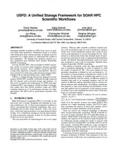
4.3 Case Study: Sweep3D Now that the system models have been validated using the matrix multiply benchmark, they can be used to predict the performance of any application executing on them given that the proper characterization and stimulus development steps have been conducted. In order to display the full capabilities and features of FASE, a more complex application was selected. The Sweep3D algorithm forms the foundation of a real Accelerated Strategic Computing Initiative (ASCI) application and solves a 1-group, time-independent, discrete ordinate 3D Cartesian geometry neutron transport problem [8, 9]. As shown in Figure 9, each iteration of the algorithm involves two main steps. The first step solves the streaming operator by ‘sweeping’ each angle of the Cartesian geometry using blocking, point-to-point communication functions while the second step uses an iterative process to solve the scattering operator employing collective functions. There are numerous input parameters that may be set including the number of processing elements in the X and Y dimensions of the logical system as well as the number of grid points (i.e. double-precision, floating-point values) assigned to the XYZ dimensions of the data cube. The default dataset sizes supplied with Sweep3D are 50 2 50 2 50 and 150 2 150 2 150, although the experiments in this section will also explore an intermediate dataset, 100 2 100 2 100. In this section, we present a set of experiments designed to quantify the accuracy and speed of the FASE simulation environment with respect to the Sweep3D application. The first experiment illustrates the accuracy of FASE by comparing experimentally measured execution times of Sweep3D versus the times produced by the corresponding simulated systems. Experiment 2 analyzes the speed of simulations conducted using FASE and demon-

strates how the speed scales with system size. The section concludes with a final experiment that showcases the full potential of the FASE framework by providing a detailed simulative analysis of the Sweep3D application running on systems of various sizes, interconnect technologies, topologies and middleware attributes. 4.3.1 Experiment 1: Accuracy The first set of experiments performed using Sweep3D was very similar to those from the previous section. The main difference, however, is that the system under study for these experiments leverages the abilities of FASE to simulate heterogeneous components. This system is composed of a heterogeneous, 64-node Linux cluster that features four types of computational nodes, as listed in Table 4. All measurements and Sequoia traces were gathered over the Gigabit Ethernet interconnect. Figure 10 shows a comparison of the execution times from the physical and simulated systems while increasing the system and dataset sizes. Table 5 displays the errors between experimental and simulative execution times. In this experiment, we observed slightly higher error rates than the matrix multiply benchmark and network validation tests, but this trend is to be expected considering the increased complexity of the Sweep3D application and heterogeneous system used for the study. In all but five cases, error rates were below 10%, with many cases showing errors around 1%. In the cases with 10% error or greater, we can largely attribute the higher values to extraneous data traffic and spurious OS activity among other effects due to non-dedicated resources. Once again, the increased error rates occurred in cases where either dataset sizes were small or system sizes Volume 83, Number 10 SIMULATION


737


Table 4. Compute node specifications for each cluster in heterogeneous system Node count

Processor

Memory

OS

Kernel

Cluster 1

10

1.4 GHz Opteron

1 GB DDR333

CentOS

2.6.9–22

Cluster 2

14

3.2 GHz Xeon with EM64T

2 GB DDR333

CentOS

2.6.9–22

Cluster 3

30

2.0 GHz Opteron

1 GB DDR400

CentOS

2.6.9–22

Cluster 4

10

2.4 GHz Xeon

1 GB DDR266

Redhat 9

2.4.20–8

Figure 10. Experimental versus simulative execution times for Sweep3D

were relatively large (or both). The maximum error observed is 23.28%, which is under the acceptable threshold for predicting performance of simulated systems since real-world implementations of the hardware and software devices will have a great effect on the actual performance of the final system. 4.3.2 Experiment 2: Speed For each experiment, the testbed execution time of the application was compared to the simulation time of the virtually-prototyped system. As seen in Figure 11, the simulation time increases with both dataset size and system size. Increases in either property raise the amount of network traffic, thus increasing the computation time for processing interactions between the higher-fidelity models. In fact, the longest simulation time (1 hr) occurred for the 64-node system using the 150 2 150 2 150 dataset. 738 SIMULATION

Table 5. Experimental versus simulation errors (%) for Sweep3D System

Dataset size

size

50 2 50 2 50 100 2 100 2 100 150 2 150 2 150

2

0.69

0.13

0.21

4

0.90

5.38

9.76

8

0.60

0.25

2.84

16

8.36

10.11

15.31

32

5.95

23.28

1.03

64

14.66

17.36

1.02

While a 1 hr simulation time is within an acceptable tolerance, if we extrapolate the timing results to even larger system and dataset sizes, we find that a system of 1024 nodes computing a 250 2 250 2 250 grid-point dataset will take approximately 70 hr. In order to cut




Figure 11. Ratios of simulation to experimental wall-clock completion time for varying system and data sizes

the time when simulating the computation of very large datasets on large-scale systems, stimulus development and simulation techniques as described in Section 3 can be employed. In this case, knowledge of the application’s execution characteristics can help to speed up simulations. The Sweep3D application performs twelve iterations of its core code, with each compute node having identical communication blocks and very similar computation blocks per iteration. The affinity across iterations allows us to use the performance data collected during a single iteration to extrapolate the total time taken to execute all twelve iterations. This process can lead to decreased simulation times with little effect on simulation accuracy. In fact, removing all but a single iteration from the Sweep3D traces resulted in a simulation speedup of 9.6 (a total of 7 min rather than 65 min) while impacting the accuracy of the model by less than 3 1%. 4.3.3 Experiment 3: Virtual System Prototyping Now that we have a fast and accurate baseline system for the Sweep3D application, we can explore the effects of changing the system configuration. This experiment explores the performance impact of increasing the number of nodes in the system by scaling the processing power of each node. This scaling effectively extrapolates the performance of the baseline 64-node system to represent the performance of Sweep3D executing on systems up to 8192

nodes. The results provided in this experiment present the best-case values of each system size since network issues such as switch congestion and multi-hop transfers, which arise from adding additional nodes to a system, are not considered. Although the actual network pressures of these systems are not fully represented, the results do provide an upper bound performance of the Sweep3D application running on the corresponding system. This upper bound can be used to quickly identify whether or not a particular system is suitable to run a particular application, thus facilitating the evaluation of numerous configurations with the intent of pinpointing a small subset of the original candidate systems to simulate in more detail. Future work will incorporate the stimulus development techniques discussed in Section 3.1.2 so that network contention is considered to improve the accuracy of the performance predictions. The various networks that we examine include standard Gigabit Ethernet (GigE), an enhanced version of GigE (10 GigE), InfiniBand, a 2D 8 2 8 direct-connect SCI network and a 3D 4 2 4 2 4 SCI network. Each configuration included in this study attempts to shed light on how changes in system size, network bandwidth, network latency, middleware characteristics and topology affect the overall performance of Sweep3D, each of which is easily configurable via the FASE framework. The results from this experiment are displayed in Figure 12 with the 64-node Gigabit Ethernet system used as the baseline. Volume 83, Number 10 SIMULATION


739


Figure 12. Execution times for Sweep3D running on various system configurations

Figure 12 shows that the Gigabit Ethernet system experienced nearly linear speedups until the system size reached 1024 nodes. At this point, the communication of Sweep3D begins to dominate execution time. In general, the trends displayed in Figure 12 were surprising, given that an initial timing analysis of the algorithm showed that half the execution time was spent in communication blocks. Upon further analysis, we determined that the reason for these trends is due to the ‘Late Sender’ problem where processes post their MPI_Recvs before the matching MPI_Send is executed by the corresponding process, causing the receiving process to become idle. In the case with 8192 nodes, the application becomes network-bound, even with the Late Sender problem. We must therefore change the focus to other network technologies to alleviate the communication bottleneck. The first attempt to remedy the communication bottleneck for larger system sizes employed optimized versions of TCP and MPI. Specifically, we increased key parameters such as TCP window size and TCP maximum transfer unit (effectively enabling the use of jumbo frames) as well as reduced MPI overhead. This case, labeled Enhanced GigE, showed little improvements in total execution time, leading us to conclude that the bandwidth and latency of the network dictate the performance of communication events rather than the middleware. The following 740 SIMULATION

tests replaced the Gigabit Ethernet interconnect with highperformance networks such as 10 GigE, InfiniBand and SCI. Figure 12 shows that in smaller systems, the interconnect has little effect on the performance of Sweep3D. However, it becomes apparent that beyond 1024 nodes, a faster interconnect provides better speedups. For example, the 10 GigE and InfiniBand interconnects offer speedups of 4.12 and 5.312, respectively, over the baseline GigE system. Figure 13 illustrates the maximum speedups for the various high-performance networks that were tested. Not only do these tests analyze the effects of adding bandwidth and lowering latency, but the SCI cases demonstrate the power of virtual system prototyping by exploring the impact of mapping the Sweep3D algorithm to drastically different topologies, specifically a 2D and 3D torus. At first glance, the Sweep3D algorithm seems to map well to direct-connect network topologies based on its nearest neighbor communication pattern1 however, from Figure 13 it appears that this is not exactly the case. Further analysis of the application and underlying architecture shows that the three fundamental characteristics of the SCI network hinder further performance improvements. First, the SCI protocol uses small payload sizes of 128 bytes which cannot effectively amortize communication overhead. The second and third characteristics are the one-way packet flow of a dimensional ring and the packet forward-




Figure 13. Maximum speedups for Sweep3D running on various network configurations

ing or dimension switching delays that occur at each intermediate node while routing packets to the destination. Under certain circumstances, as dictated by the Sweep3D algorithm, few packets experience more than one forwarding delay due to the target node being the next neighboring node in the dimensional ring’s packet flow. This case provides optimal mapping between the algorithm and the network architecture, resulting in excellent performance. However, this scenario is only one of four communication flows used by Sweep3D. The remaining communications result in numerous transactions that must travel almost the entire length of a dimensional ring in order to reach its destination, resulting in many multi-hop transfers, higher latencies and lower overall speedups. These negative effects could easily be lost when using low-fidelity analytical network models due to their inability to capture structural characteristics that can greatly impact overall system performance. Not only can FASE be used to analyze the effects of interchanging network technologies, but it can also provide a highly detailed analysis of a specific technology. We chose the InfiniBand network for the in-depth study since it showed the best performance of the six configurations. The InfiniBand model, as well as the MPI middleware model, has numerous user-definable parameters that can be changed to correspond to the current and future versions of the technologies. These parameters provide a mechanism to perform fine-grained analyses to squeeze as much performance as possible from a specific technology while also providing valuable insight

into any new bottlenecks that may arise during future upgrades. From the results in Figure 14, one can see that even at 8192 nodes, network enhancements have little effect on the performance of the InfiniBand system. The greatest speedup from changes in the communication layer comes from middleware enhancements that achieve a 1.212 performance boost over the baseline. These results indicate that further improvements of the InfiniBand system’s computation capabilities are needed in order to show any significant speedups when tweaking the middleware and network layers. The enhancement that increases network and processing performance as well as decreases the overhead associated with the middleware (see Figure 14, Middleware+Network+Processor enhancement) reinforces this claim by providing a 2.442 speedup. This study only provides a brief summary of the modifications that can be made to test the effectiveness of key technologies when analyzing an application using FASE. 5. Related Work Predicting the performance of an arbitrary application executing on a specific system architecture has been a longsought goal for application and system designers alike. Throughout the years, researchers have designed a number of prediction frameworks that employ varying techniques and methodologies in order to produce accurate and meaningful results. The approach taken by each framework allows it to overcome certain obstacles or focus on specific Volume 83, Number 10 SIMULATION


741


Figure 14. Speedups for Sweep3D running on 8192-node InfiniBand system

application or system types while inevitably sacrificing some key feature such as accuracy, speed or scalability. The following paragraphs briefly describe existing prediction environments similar to FASE, and the methodologies and general limitations of each. The Integrated Simulation Environment (ISE) [10], a precursor to FASE, employs hardware-in-the-loop (HWIL) simulation in which actual MPI programs are executed using real hardware coupled with high-fidelity simulation models. The computation time of each simulated node is calculated via a process spawned on a ‘process machine’, while network models calculate the delays for the communication events. Although the ISE shows reasonable simulation time and accuracy, the scalability of the framework is limited due to the large number of processes needed to represent large-scale systems. The Performance Oriented End-to-end Modeling System (POEMS) project [11] adheres to an approach similar to the HWIL simulation in that systems can be evaluated based on results from actual hardware and simulation models as well as performance data collected from actual software and analytical models. The simulation environment used by POEMS integrates SimpleScalar with the COMPASS simulator [12] enabling direct execution-driven parallel simulation of MPI programs. These high-fidelity simulators can provide very accurate and insightful results, although the simulations can require large amounts of time especially when dealing with very large systems. 742 SIMULATION

While ISE and POEMS use execution-driven simulations, other projects employ a model-driven approach. CHAOS [13] creates application emulators that reproduce the computation, communication and I/O characteristics of the program under study. The emulators are then used to pass their information to a suite of simulators that, in turn, determine the performance of the modeled application on the target simulated system. The PACE [14] framework defines a custom language called Characterization Instrumentation for Performance Prediction of Parallel Systems (CHIP3 S) that is used to generate a model describing a parallel program’s flow control and workload. Similarly, Performance Prophet [15] uses the Unified Modeling Language (UML) to model parallel and distributed applications. Both PACE and Performance Prophet use these models to drive systems composed of both analytical and simulation models in order to balance speed and accuracy. Due to the inherent difficulty of automatically creating an accurate application model, all three projects require intimate knowledge of the program it represents. As a result, the source code must be analyzed and profiled to collect the necessary information to reconstruct the program’s execution. Work conducted by the Performance Evaluation Research Center (PERC) focuses on performance prediction of parallel systems under the assumption that an application’s performance on a single processor is memory bound and the interconnect dictates the scalability of the pro-




gram under study [16, 17]. The framework uses a threestep process: 1. collect memory performance parameters of the considered machine1 2. collect memory access patterns independent of the underlying architecture on which the application is executed1 and 3. algebraically convolve the results from steps (1) and (2), then feed the results to the DIMEMAS [18] network simulator developed at the European Center for Parallelism of Barcelona. The researchers of PERC have reported accurate performance predictions using a wide range of applications. However, collecting memory access patterns can be a very time consuming task that results in large amounts of data for each application considered. Also, the DIMEMAS network simulator is relatively simplistic and has the potential for large inaccuracies when analyzing communication-intensive applications with potential contention issues. Performance prediction is the main theme of FASE and the frameworks mentioned above. However, performance analysis is an integral technique used to characterize the applications under study prior to simulation. The accuracy and detail of this characterization data can greatly influence the accuracy and speed of the simulation frameworks that use it. While a great number of performance analysis tools exist for various purposes [19], SvPablo [20], Paradyn [21] and TAU [22] are the tools most applicable to the FASE simulation framework. SvPablo may be used to analyze the performance of MPI and OpenMP parallel programs, allows for interactive instrumentation and correlates performance data with the original source code. Paradyn is also compatible with MPI programs and offers the advantage that no modifications to the source code are needed due to dynamic instrumentation at the binary level. Paradyn’s focus is on the explicit identification of performance bottlenecks. TAU is an MPI performance analysis tool that can provide performance data on a thread-level basis and provides the user with a choice of three different instrumentations. Many performance analysis tools including SvPablo and TAU are based on, or support, the popular PAPI, which is also supported by the Sequoia tool used by FASE. Each of these analysis tools can be incorporated into the pre-simulation stage of FASE in conjunction with or as a replacement for Sequoia to provide additional information on an application’s behavior. FASE culminates many of these general techniques and methods in order to provide a robust, flexible performance prediction framework. In addition, FASE features an environment that allows users to build virtual representations of candidate architectures. These virtual prototypes

capture structural dependencies such as network congestion and workload distribution that can greatly impact an application’s performance. For example, the applicationmapping issue of Sweep3D executing on the SCI-based system, discussed in Section 4.3.3, demonstrates performance problems arising from how the application exercises the underlying topology and network protocol. Many of the frameworks described in this section use simplistic communication models that have difficulties capturing such issues. Furthermore, FASE employs a systematic, iterative methodology that produces highly modular application characterization data and component models. The framework illustrates the relationships between the application performance information and the architectural models such that features and mechanisms within the models can be identified and altered to improve prediction accuracy and simulation speed. The other frameworks propose using models of various fidelities in order to speed up the simulations1 however, they do not explicitly describe the decision-making process of choosing or designing a model’s fidelity. Finally, FASE provides a fully extensible pre-built model library with components ranging from the application layer down to the hardware layer. Unlike many of the frameworks described above, FASE includes a number of detailed middleware models that can have significant impacts on the performance of the overall system. Many of the pre-built models are highly tunable, thus allowing a single, generic model to represent many different implementations based on the parameter values set by the user. The combination of these features makes FASE a powerful, flexible environment for rapidly evaluating applications executing on a variety of candidate systems. 6. Conclusions and Future Work The task of designing powerful yet cost-efficient HPC systems is becoming extremely daunting due not only to the increasing complexity of individual computation and I/O components, but also to the effective mapping of grandchallenge applications to the underlying architecture. In this paper, we have presented a framework called the Fast and Accurate Simulation Environment (FASE) that aids system engineers overcome the challenges of designing systems that target specific applications through the use of analysis tools in conjunction with discrete-event simulation. Within the application domain, FASE provides a methodology to analyze and extract an application’s performance-critical data which is then used to discover trends and limitations as well as provide stimuli for simulation models for virtual prototyping. In this paper, we provided background on various options for performance prediction of HPC systems through modeling and simulation, and outlined the need for a solution that can provide fast simulation times with accurate results. The FASE framework was then outlined and its different components and features were described. Volume 83, Number 10 SIMULATION


743


In order to showcase the capabilities of FASE, we gathered a variety of results showing the performance of various system configurations. We first provided validation results for our InfiniBand, TCP/IP over Ethernet and SCI models, showing that the network models that serve as the backbone of the case studies in this paper have been carefully tuned to accurately match real hardware. We then showed the results of a matrix multiply case study where we compared experimental to simulated execution times for a parallel MPI-based matrix multiply benchmark. In most cases, errors in the models were less than 1%, with the maximum error of 12.7% occurring in a case with a small dataset size and a large system size. These conditions result in short experimental runtimes of less than one second where transient effects such as OS task management and page faults can cause unpredictable deviations in application execution time. In terms of simulation speed, the slowdowns observed by simulating the parallel matrix multiply were very low, and in some cases the simulation actually completed before the actual system finished executing the code. The final case study presented a series of experiments using the Sweep3D benchmark, which is the main kernel of a real Accelerated Strategic Computing Initiative application. We performed simulation and hardware experiments over a range of dataset sizes using a Gigabit Ethernet-based system, and again found errors to be very low in most cases. A maximum error of 23.28% was observed, which is considered acceptable when dealing with predicting the performance of a complex application running on an HPC system. Again, the cases with high errors correspond to non-typical HPC scenarios with larger systems working on small datasets resulting in conditions that amplify deviations in experimentally measured runtimes. We also proposed and employed tactics to speed up simulation by 102 while sacrificing less than 1% accuracy. With a fast and accurate baseline system established for Sweep3D, we proceeded to use the FASE methodology to predict the performance of the application for systems with various sizes and network technologies. We found that the application was actually more processorbound than initially anticipated due to the MPI ‘Late Sender’ problem. A process posts an MPI_Recv before the corresponding MPI_Send is executed, causing the receiving process to become idle. However, as the systems increased in size, Sweep3D became network bound, with 10 Gigabit Ethernet and InfiniBand both providing significant performance improvements over the Gigabit Ethernet baseline mainly due to their increased bandwidth. The analysis of Sweep3D concluded with an in-depth look at its execution on an InfiniBand system while varying fine-grained parameters such as network bandwidth, packet size and middleware overhead. These modifications provided minimal performance improvements because the algorithm’s bottleneck changed from communication to computation when network backpressure was reduced by choosing an improved network tech744 SIMULATION

nology (i.e. InfiniBand). Following the case studies, we presented other research related to the FASE framework in terms of performance analysis, modeling and prediction. Some of the many directions for future research for the FASE project include expanding the capabilities of the procedures in the application domain with scalability and automation in mind. One area of expansion is to include tools from other research projects to accommodate more in-depth computation modeling, disk I/O, operating system interactions and incorporating execution models for exotic hardware components. In addition, the components in the FASE library will be expanded to incorporate the additional information provided to the simulation models by these tools. A specific scalability issue that must be addressed in the application domain is stimulus generation for virtually-prototyped systems many times larger than those physically available. The process and extrapolation methods discussed in Section 3.1.1 must be explored in more depth regarding their abilities to provide complete and accurate data that can be employed by the simulation models. Future work in the simulation domain includes developing a comprehensive approach to calibrate component models that may include a benchmark suite to automatically tailor components to pre-existing systems. Also, the speed and accuracy of FASE’s system analysis step will be improved through the use of a hierarchical simulation approach and the inclusion of a measure of randomness to capture variations inherent in the measurement of computer systems, respectively. 7. References [1] Vetter, J., N. Bhatia, E. Grobelny, and P. Roth. 2005. Capturing Petascale Application Characteristics with the Sequoia Toolkit. In Proceedings of Parallel Computing 2005. Malaga, Spain, September 13–16, 2005. [2] MPI Forum. 1995. MPI: A Message-Passing Interface Standard. University of Tennessee, Version 1.1. [3] Browne, S., J. Dongarra, N. Garner, K. London, and P. Mucci. 2000. A Scalable Cross-Platform Infrastructure for Application Performance Tuning Using Hardware Counters. In Proceedings of SC2000. Dallas, Texas, November 4–10, 2000. [4] Grobelny, E. and J. Vetter. 2006. Extrapolating Communication Patterns of Large-scale Scientific Applications. Technical Report, University of Florida and Oak Ridge National Laboratory, 2006. [5] Schorcht, G., I. Troxel, K. Farhangian, P. Unger, D. Zinn, C. Mick, A. George, and H. Salzwedel. 2003. System-Level Simulation Modeling with MLDesigner. In Proceedings of 11th IEEE/ACM International Symposium on Computer and Telecommunication Systems (MASCOTS). Orlando, Florida, October 12–15, pp. 207– 212. [6] Zaki, O., E. Lusk, W. Gropp, and D. Swider. 1999. Toward Scalable Performance Visualization with Jumpshot. International Journal of High Performance Computing Applications 13(2), 277–288. [7] Gustavson, D., and Q. Li. 1996. The Scalable Coherent Interface (SCI). IEEE Communications 34(8), 52–63. [8] Koch, K., R. Baker, and R. Alcouffe. 1992. Solution of the FirstOrder Form of the 3-D Discrete Ordinates Equation on a Massively Parallel Processor. Transactions of the American Nuclear Society 65: 198.




[9] Vetter, J. and A. Yoo. 2002. An Empirical Performance Evaluation of Scalable Scientific Applications. In Proceedings of SC2002. Baltimore, Maryland, November 16–22. [10] George, A., R. Fogarty, J. Markwell, and M. Miars. 1999. An Integrated Simulation Environment for Parallel and Distributed System Prototyping. Simulation 72(5), 283–294. [11] Deelman, E., A. Dube, A. Hoisie, Y. Luo, R. Oliver, D. SundaramStukel, H. Wasserman, V. Adve, R. Bagrodia, J. Browne, E. Houstis, O. Lubeck, J. Rice, P. Teller, and M. Vernon. 2000. POEMS: End-to-End Performance Design of Large Parallel Adaptive Computational Systems. IEEE Transactions on Software Engineering 26(11), 1027–1048. [12] Bagrodia, R., E. Deelman, S. Docy, and T. Phan. 1999. Performance Prediction of Large Parallel Applications Using Parallel Simulations. In Proceedings of 7th ACM SIGPLAN Symposium on Principles and Practice of Parallel Programming. Atlanta, Georgia, pp. 151–161. [13] Uysal, M., T. Kurc, A. Sussman, and J. Saltz. 1998. A Performance Prediction Framework for Data Intensive Applications on Large Scale Parallel Machines. Technical Report CS-TR-3918 and UMIACS-TR-98-39, University of Maryland, Department of Computer Science and UMIACS. [14] Cao, J., D. Kerbyson, E. Papaefstathiou, and G. Nudd. 2000. Performance Modeling of Parallel and Distributed Computing Using PACE. In Proceedings of 19th IEEE International Performance, Computing, and Communications Conference. Phoenix, Arizona, pp. 485–492.

[15] Pllana, S., and T. Fahringer. 2005. Performance Prophet: A Performance Modeling and Prediction Tool for Parallel and Distributed Programs. In Proceedings of 2005 International Conference on Parallel Processing. Oslo, Norway. [16] Snavely, A., L. Carrington, and N. Wolter. 2002. Framework for Performance Modeling and Prediction. In Proceedings of SC2002. Baltimore, Maryland, November 16–22. [17] Bailey, D., and A. Snavely. 2005. Performance Modeling: Understanding the Present and Predicting the Future. In Proceedings of Euro-Par 2005. Lisbon, Portugal, August 30–September 2. [18] Badia, R., J. Labarta, J. Gimenez, and F. Escale. 2003. DIMEMAS: Predicting MPI Applications Behavior in Grid Environments. In Proceedings of Workshop on Grid Applications and Programming Tools (GGF8). Seattle, Washington, June 25. [19] Moore, S., D. Cronk, K. London, and J. Dongarra. 1998. Review of Performance Analysis Tools for MPI Parallel Programs. Technical Report, University of Tennessee, Computer Science Department, 1998. [20] DeRose, L., and D. Reed. 1999. SvPablo: A Multi-Language Architecture-Independent Performance Analysis System. In Proceedings of International Conference on Parallel Processing. Fukushima, Japan, September. [21] Miller, B., M. Callaghan, J. Cargille, J. Hollingsworth, R. Irvin, K. Karavanic, K. Kunchithapadam, and T. Newhall. 1995. The Paradyn Parallel Performance Measurement Tool. IEEE Computer 28(11), 37–46. [22] Shende, S., and A. Malony. 2006. The TAU Parallel Performance System. International Journal of High Performance Computing Applications 20(2), 287–331.



745

FASE: A Framework for Scalable Performance Prediction of HPC ...

FASE: A Framework for Scalable Performance Prediction of HPC ...

Suggest Documents

performance prediction for hpc on clouds

A Framework for Scalable, Parallel Performance Monitoring

A Framework for Performance Projections of HPC ...

A Framework for Performance Projections of HPC ... - CiteSeerX

A Performance Prediction Framework for Scientific ... - CiteSeerX

A Component Framework for HPC Applications - LaBRI

A Scalable Performance Prediction Heuristic for ... - Greg Stitt

Scalable HPC Workflow Infrastructure for Steering Scientific ...

developing a framework for prediction of human performance ... - aircc

A framework for Performance Prediction of Service-Oriented Architecture

A Framework for Performance Monitoring, Modelling and Prediction of ...

A Performance Prediction Framework for Data Intensive ... - CiteSeerX

Performance Prediction Techniques for Scalable Large ... - IEEE Xplore

A Runtime Framework for Energy Efficient HPC Systems Without a ...

A Scalable Framework for Information Visualization - CiteSeerX

A scalable framework for multimedia knowledge ... - CiteSeerX

A Framework for Scalable Biophysics-based Image

GLADE: A Scalable Framework for Efficient Analytics

Scalable extensible middleware framework for

A Unified Storage Framework for SOAR HPC Scientific ... - UCF CS

Cloud Computing Based HPC: A Framework for Ethiopian ... - IJIRCCE

Towards a Comprehensive Framework for Telemetry Data in HPC ...

A Runtime Framework for Energy Efficient HPC Systems ... - HAL-Inria

Towards a Comprehensive Framework for Telemetry Data in HPC ...