In this paper we construct a framework that enables us to make class predictions about telecommunication companies' financial performances. We have two ...
A FRAMEWORK FOR PREDICTIVE DATA MINING IN THE TELECOMMUNICATIONS SECTOR Adrian Costea Turku Centre for Computer Science and IAMSR / Åbo Akademi University Lemminkäisenkatu 14 B, FIN-20520 Turku, Finland
Tomas Eklund Turku Centre for Computer Science and IAMSR / Åbo Akademi University Lemminkäisenkatu 14 B, FIN-20520 Turku, Finland
Jonas Karlsson IAMSR / Åbo Akademi University Lemminkäisenkatu 14 B, FIN-20520 Turku, Finland
ABSTRACT In this paper we construct a framework that enables us to make class predictions about telecommunication companies’ financial performances. We have two goals: to validate our methodology and, using it, to gain insights in this relatively new and very sensitive industry: the telecommunications sector. We have obtained high accuracy rates for the classification models, and small differences between training and test dataset accuracy rates. The two classification techniques have performed similarly in terms of accuracy rates (decision tree, slightly better than logistic regression) and class predictions (all companies selected were placed in the same clusters by both methods). We have analyzed the movements of the largest four telecommunications companies. The results show a strong connectivity with what had really happened to these telecommunication companies during the second part of the last decade, and the beginning of the current one. KEYWORDS SOM algorithm, class predictions, telecommunication sector
1. INTRODUCTION The growth of the Internet has placed nearly boundless amounts of information at our disposal. This amount greatly exceeds our capacity to analyze it. One of the areas greatly affected by the development of the Internet is financial analysis. There are enormo us amounts of financial data available to anyone on the Internet, the only problem being that we often lack tools to quickly and accurately process these data. Managers and stakeholders are increasingly looking to knowledge discovery in databases (KDD) for new tools (Adriaans & Zantinge, 1996). Tools of this type could interestingly be applied to rapidly changing industries, in order to get an overview of the situation. One such market is the international telecommunications industry. In the last decade a dramatic change in the ownership structure of telecommunications companies has taken place, from public (state-owned) monopolies to private companies. The rapid development of mobile telephone networks and video and Internet technologies has created enormous competitive pressure on the companies. As new competitors arise, companies need intelligent tools to gain a competitive advantage. Also, stock market expectations are enormous, and investors and financial analysts need tested tools to gain information about
38
A FRAMEWORK FOR PREDICTIVE DATA MINING IN THE TELECOMMUNICATIONS SECTOR
how companies perform financially compared to their competitors, what they are good at, who the major competitors are, etc. (Karlsson et al., 2001). In this paper we apply a new methodology to classify telecommunications companies in respect to their financial performance. First we use the SOM (Self-Organizing Map) algorithm to cluster the companies, constructing a two-dimensional unified-distance matrix map (a two-dimensional representation technique for the distance between neurons) (Ultsch & Siemon, 1990). We then attach the class labels to each data row from the dataset and apply two classification methods to develop class prediction models. As is presented in (Rudolfer et al., 1999) the two classification methods (multinomial logistic regression and decision tree algorithm) performed similarly, in terms of their accuracy rates. As a conclusion of this research, we now want to be able to validate our methodology against a dataset consisting of financial data on telecommunications companies. Here we focus more on understanding how different financial factors can and do contribute to the companies’ movements from one group/cluster to another. We base our research on a previous study (Karlsson et al., 2001), in which the author uses the SOM to evaluate the financial performance of telecommunications companies. The problem with this approach is that we basically have to train new maps, or standardize the new data according to the variance of the old dataset, in order to add new labels to the maps. Inserting new data into an existing SOM model becomes a problem when the data have been standardized, for example, within an interval like [0,1]. Also, the retraining of maps requires considerable time and expertise. In this paper we go one step further and build a model that enables us to predict how the companies would be classified by a particular SOM model. We propose that our methodology solves these problems associated with adding new data to an existing SOM cluster model. The rest of the paper is organized as follows. In section 2 we briefly present our new methodology to model the relationship between some financial variables of telecommunications companies and their financial performance classifications. In the following section we present the results of clustering phase, and then in section 4, the two classification models are applied and compared. In section 5 we analyze the results using the data for some companies in 2000 and 2001, and compare them with the results of the SOM model. In the final section we present our conclusions.
2. SHORT DESCRIPTION OF THE METHODOLOGY Our methodology consists of two phases: a clustering phase, in which we obtain several clusters that contain similar data-vectors in terms of Euclidean distances, and a classification phase, in which we construct a class predictive model in order to place the new row data within the clusters obtained in the first phase as they become available. There are several clustering methods available, and they can be divided into two categories: hierarchical and non-hierarchical. Hierarchical clustering can be further divided into splitting and merging techniques. In the case of merging hierarchical clustering, each input data-vector is first associated with a cluster. Then, a measure is used to calculate the distance between all clusters. The two clusters that are closest to each other are then merged. These steps are repeated until one single cluster is obtained. For further information on different clustering techniques and how they work, see (Vesanto & Alhoniemi, 2000). Non-hierarchical (partitive) clustering techniques directly divide the data into clusters so that the intra-cluster distance is minimized and inter-cluster distance is maximized (Tan et al., 2002). Among clustering techniques, the SOM (a non-hierarchical clustering technique) has the advantages of good visualization and low computational cost. In (Kohonen et al., 2000) the SOM was used to train a 500-dimension dataset (6.8 million data rows). In the classification phase we want to build a model that describes one categorical variable (our performance class) against a vector of dependent variables (in our case: the financial ratios). Three approaches to building real classifiers are presented in the literature (Hand et al., 2001): the discriminative approach, the regression approach and the class-conditional approach. The two classification techniques used in this paper belong to the regression approach. The decision tree algorithm can be included in both discriminative or regression approaches, depending upon how it is set up: if the tree provides the posterior class probability distribution at each leaf (regression approach) or the tree provides only the predicted class at each leaf (discriminative approach). The decision tree software tool that we use (See5 software developed by Quinlan’s research team – http://www.rulequest.com/ ) supports regression approach in the sense that it calculates these posterior probabilities for each new data row.
39
IADIS International Conference WWW/Internet 2002
The different steps included in our methodology are presented below. Steps for the clustering phase: · preprocessing of initial data, · training using the SOM algorithm, · choosing the best map, and · identifying the clusters and attaching outcome values to each data row. Steps for the classification phase using multinomial logistic regression: · developing the analysis plan, estimation of logistic regression, · assessing model fit (accuracy), · interpreting the results, and · validating the model. Steps for the classification phase using the decision tree algorithm: · constructing a decision tree using a classifier, · assessing model accuracy, · interpreting the results, and · validating the model. This methodology was applied on Karlsson et al.’s (2001) financial dataset that consists of 462 data rows. The dataset contains 88 companies from five different regions: Asia, Canada, Continental Europe, Northern Europe, and USA, and consists of seven financial ratios per company per year. The ratios used were: operating margin, return on equity, and return on total assets (profitability ratios); current ratio (liquidity ratio); equity to capital and interest coverage (solvency ratios); and receivables turnover (efficiency ratio). The ratios were chosen from Lehtinen’s (1996) comparison of financial ratios’ reliability and validity in international comparisons. The data used to calculate the ratios were collected from companies’ annual reports, using the Internet as the primary medium. The time span is 1995-1999. We use data for the years 2000 and 2001 to test our classification models.
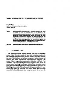
3. APPLYING SOM The SOM algorithm is a well-known unsupervised-learning algorithm developed by Kohonen in early 80’s. A comprehensive explanation of this algorithm and its software implementation can be found in (Kohonen, 1997; Kohonen et al., 1996). When training the maps with SOM we followed the same procedure as in (Karlsson et al., 2001). First of all, in order to avoid the algorithm placing too much emphasis on extreme values, we have limited the range of the all variables to –50, 50. Then, the data were standardized using several standardization methods: the standard deviation of the entire dataset, the standard deviation of each individual variable, the variance of the entire dataset, and the variance of each individual variable. Different values for SOM parameters were tested on the four obtained datasets. Finally, we chose the variance of the entire dataset as the standardization method due to better maps in terms of their readability. The final map average quantization error was: 0.039245. The chosen U-matrix (Unified-distance) map and its clearly identifiable clusters are presented below (Figure 1):
Figure 1. (a) The final 9x6 U-matrix map (1995-99 data) and (b) the identified c lusters on the map
40
A FRAMEWORK FOR PREDICTIVE DATA MINING IN THE TELECOMMUNICATIONS SECTOR
In order to define the different clusters features planes were analyzed as well as the row data. By analyzing the feature planes one can easily discover how well the companies have been performing according to each financial ratio. Dark colors of neurons on a feature plane correspond to low values for that particular variable, while light colors correspond to higher values. In our particular case, all of the variables are positively correlated with company performance (higher values for variables imply good performance by the company and vice versa). The class variable that we add to the dataset for each data row is in this case measured on an ordinal scale, rather then on an interval one. This means that the classes (A 1 , A2 , B, C1 , C2 , D) are in descending order in terms of companies’ financial performance, but they are not equally distributed (the distances among different classes are different). A short explanation of the characteristics of each group/cluster is presented below: Group A1 – corresponds to the best performing companies (profitability very good, solvency decent, liquidity slightly worse). Group A2 – the second best performing group (slightly lower profitability than Group A 1, strong liquidity and solvency). Group B – includes companies with slightly poorer financial performance than the A groups (good profitability, especially ROE ratio, poorer liquidity and solvency than A companies). Group C1 – indicates decent profitability, good liquidity, poorer solvency and efficiency (Interest Coverage and Receivables Turnover). Group C2 – is slightly poorer than the C1 group. It contains companies with decent profitability, poor liquidity, and poor solvency and efficiency ratios. Group D – the poorest group: poor profitability and solvency, average liquidity. It mainly contains service providers from Europe and USA, and Japanese companies in 98-99 (due to the Asian financial crisis that peaked in 1997-98). After we chose the final map, and identified the clusters, we attached class values to each data row as follows: 1 – A 1, 2 – A 2, 3 – B, 4 – C1, 5 – C2, 6 – D. In the next section we will construct two different classification models to classify the data for the years 2000-01 into already existing clusters. We will compare the two models in terms of their accuracy rates and class prediction performances. When constructing the maps (.cod files) we have used a built-in Windows software program, developed by one of the authors, which is based on SOM_PAK C source files that are available at http://www.cis.hut.fi/research/som_pak/. Nenet v1.1a, available for free-demo download at http://koti.mbnet.fi/~phodju/nenet/Nenet/Download.html, was used to visualize the “.cod” files.
4. APPLYING THE TWO CLASSIFICATION TECHNIQUES A more detailed presentation of each classification technique (multinomial logistic regression – MLR and decision tree induction – DTI) can be found in (Rudolfer et al., 1999). Here we will apply our methodology presented in section 2 and try to validate it. Firstly, multinomial logistic regression was applied on the dataset (updated with values for the class variable, i.e. the associated cluster from the SOM). Our research problem was to find a relationship between a categorical variable (financial performance class) and a financial data-vector. We had no problems regarding requirements about size and missing data in our dataset. The SPSS software package was used to perform the logistic regression. To see how well the model fits the data we look at the “Model Fitting information” and “Pseudo R-Square” output tables of SPSS (chi-square value has a significance of < 0.0001 and Nagelkerke R2 = 0,978). This means that there is a strong relationship between the class variables and the financial ratios (97,8% of the class variation is explained by variations in input variables). To evaluate the accuracy rate of 92,4%, we used two criteria (to calculate two new accuracy rates): the proportional by chance and maximum by chance accuracy rates (Hair, Anderson, & Tatham, 1987, p. 89-90). Table 1. Evaluate the model’s accuracy
Model Telecom
92,4%
Proportional by chance criterion 17,83%
Maximum by chance criterion 24,5%
41
IADIS International Conference WWW/Internet 2002
The model accuracy rate is validated against both criteria (it exceeds both standards: 1,25 * 17,83% = 22,3% and 1,25 * 24,5% = 30,62%). To interpret the results of our analysis, we study the “Likelihood Ratio Test” and “Parameter Estimates” output tables of SPSS. All variables are significant (p < 0.01), except “Current Ratio” (p = 0.16), which means that this variable doesn’t have a strong contribution to explaining class predictions. However, keeping this variable will not harm our model. Not all coefficients for all regression equations are statistically significant. By looking at columns “B” and “exp(B)” from the “Parameter Estimates” output table, we can determine the direction of the relationship and the contribution to performance classification of each independent variable. The findings are as expected e.g.: the likelihood that one data row will be classified into group A1 is positively correlated with profitability and solvency ratios and, slightly, negatively correlated with liquidity and efficiency ratios. This corresponds with the characteristics of group A 1 (findings of Karlsson et al. (2001)). We validate our MLR model by splitting the data into two parts of the same size (231 data-rows). When we have used first part (“split” = 0) as training sample, we have used the second one as test sample, and vice versa. The results are presented in Table 2.
Telecom
Table 2. Datasets’ accuracy rates and accuracy rates estimators when applying multinomial logistic regression
Model Chi-Square (p < 0,0001) Nagelkerke R2 Learning Sample Test Sample Significant coefficients (p