Proceedings of the ASME 2014 International Design & Engineering Technical Conferences and Computers & Information in Engineering Conference IDETC/CIE 2014 August 17-20, 2014, Buffalo, New York, USA
DETC2014-35041
A FRAMEWORK FOR PROBLEM STANDARDIZATION AND ALGORITHM COMPARISON IN MULTIBODY SYSTEM
Ying Lu∗ Jedediyah Williams Jeff Trinkle The RPI Robotics Laboratory Department of Computer Science Rensselaer Polytechnic Institute Troy, New York, 12180 Email:
[email protected]
` Claude Lacoursiere HPC2N/UMIT Research Laboratory Umea˚ University ˚ 90187 Umea, Sweden
[email protected]
ABSTRACT The underlying dynamic model of multibody systems takes the form of a differential Complementarity Problem (dCP), which is nonsmooth and thus challenging to integrate. The dCP is typically solved by discretizing it in time, thus converting the simulation problem into the problem of solving a sequence of complementarity problems (CPs). Because the CPs are difficult to solve, many modelling options that affect the dCPs and CPs have been tested, and some reformulation and relaxation options affecting the properties of the CPs and solvers have been studied in the hopes to find the “best” simulation method. One challenge within the existing literature is that there is no standard set of benchmark simulations. In this paper, we propose a framework of Benchmark Problems for Multibody Dynamics (BPMD) to support the fair testing of various simulation algorithms. We designed and constructed a BPMD database and collected an initial set of solution algorithms for testing. The data stored for each simulation problem is sufficient to construct the CPs corresponding to several different simulation design decisions. Once the CPs are constructed from the data, there are several solver options including the PATH solver, nonsmooth Newton methods, fixed-point iteration methods for nonlinear problems, and Lemke’s algorithm for linear problems. Additionally, a user-friendly interface is provided to
∗ Address
all correspondence to this author.
add customized models and solvers. As an example benchmark comparison, we use data from physical planar grasping experiments. Using the input from a physical experiment to drive the simulation, uncertain model parameters such as friction coefficients are determined. This is repeated for different simulation methods and the parameter estimation error serves as a measure of the suitability of each method to predict the observed physical behavior.
NOMENCLATURE q Generalized positions of all the bodies ν, q˙ Generalized velocities of all the bodies λn Normal contact forces in the local frame λf Frictional contact forces in the local frame λt , λo Orthogonal decomposition of λf on the frictional plane in the local frame, ut Frictional contact velocity in the local frame uo Frictional contact velocity in the local frame, orthogonal to ut Gn Jacobian matrix that transforms the normal contact force from local frame to the world frame Gf Jacobian matrix that transforms the tangential contact force from local frame to the world frame 1
c 2014 by ASME Copyright
G
Jacobian matrix that transforms contact force from local frame to the world frame U Diagonal matrix with its diagonal entry equal to frictional coefficient of each contact ψn Normal gap distance between two bodies that form contacts M Generalized mass inertia matrix λapp Generalized externally applied force s Sliding speed at contact points φ(x) NCP reformulation functions ⊥ Denotes orthogonality, where a, b ∈ Rn , and a ⊥ b means aT b = 0 n ◦ Denotes the Hadamard product: where a, b ∈ R , and a ◦ a1 b1 a2 b2 b= . .. an bn
begun to develop suites of benchmark problems [21–25]. M. Gonzalez et al [22] proposed a benchmarking system for multibody system (MBS) simulation tools to compare the performance of the different available simulation methods. A collaborative benchmarking framework is provided by [23] with an online repository of test problems with reference solutions and standardized procedures and a prototype implementation of a webbased application to share the results from different methods. It aims to compare the performance of various simulators through full multi-step simulations in order to discover the best combinations of formulation, integration method, and implementation. However, little information regarding the iterative level results of a solver is provided in this framework, which prevents users from making comparisons of performance of different solvers at this low level. Previous work on building a test suite for rigid body dynamics problems was done by the Siconos group in 3DFCLib [24], where benchmark problems were stored by saving the matrices and vectors defining the specific CPs used in the Siconos simulator. Although the data hierarchy is simple and clean, there is not sufficient information from the database to reformulate the problems except as LCPs. Therefore, there is no way to compare the solvers applicable to Nonlinear CPs (NCPs).
INTRODUCTION Simulation of multibody systems is important for analysis and design in a number of areas in science and engineering. Roboticists have used it to plan complex robot behaviors such as grasping and manipulation [1, 2], to study the locomotion of sand-swimming lizards [3], and the motion of 3-D snake robots [4]. Engineers have used it to predict the performance of complex devices such as car engines [5] and scientists have used it to study rock slides [6]. The main reasons that rigid body simulation has not yet been widely embraced (beyond physics-based computer games) are inadequate speed and unproven accuracy. There is limited theoretical guidance for the design of solution algorithms for the type of CPs that must be solved at each time step. When the matrix A in the linearized CPs (LCP) is symmetric and positive semi-definite (SPSD), the vector b in the LCP [7] lies in the column space of the matrix in the CPs and there are good optimization-based polynomial time algorithms for solving them [7]. While LCPs with SPSD matrix A are known to have solutions [8,9], the matrix A in multibody system usually doesn’t have such good properties. Lemke’s algorithm [7], the PATH solver [10], nonsmooth Newton method [11–14], PGS method [15], fixed-point iteration method [16], projected Jacobi method [7, 15], implicit nonlinear method [17], and two stage methods using combinations [18–20] have not been thoroughly and fairly compared. Testing of these numerical methods is usually conducted with a small number of synthetic CPs generated to have similar properties as CPs as they would arise in simulation, but it is difficult to do this accurately. What is needed is a large set of a wide range of benchmark problems of various sizes and properties. Good benchmarking has been used for many years to assess the performance of computers and software tools. However, only recently have researchers in multibody dynamics and robotics
The goal of this paper is to set forth a new framework for fairly testing solution algorithms on a broader set of problems extracted from experiments and simulations. In our Benchmark Problems for Multibody Dynamics (BPMD) framework, we save the data needed to construct any of the typical CPs in use. This facilitates comparison of possible choices regarding modelling coordinates, dynamics formulations, the integration schemes, and the algorithms that solve the CPs. To ensure full coverage of problems of interest to the community, the BPMD framework facilitates contributions to the benchmark problem set. We believe that such a framework is critically important to the advancement of the field of rigid body dynamic simulation, because of the need of a fair way to compare performance of available solution algorithms and the lack of theoretical results to guide further algorithm development. In the first section, we present an overview of choices regarding modelling coordinates, as well as dynamic formulations for multibody dynamics. Next, we introduce the solvers available in the BPMD framework along with the formulations to which the solvers are applicable. These two parts define the platform with which algorithms may be compared. The following section describes the BPMD framework structure that we use to collect data from physics engines and how to use the BPMD database to import or export data from or to physics engines in a standard way. Finally, the accuracy of the solvers are further validated with the data from physical planar grasping experiments and the results are displayed and analysed. 2
c 2014 by ASME Copyright
FORMULATIONS AND SOLVERS There are several formulations and solvers available in BPMD framework, which are listed in Table 1. Of all the solves, Lemke’s algorithm is a pivoting method and the others are iterative.
where f (x) is a function of x. When f (x) is a linear function of x, we call it Linearized Complementarity Problem (LCP). If f (x) is a nonlinear function of x, it is named Nonlinear Complementarity Problem (NCP). The NCP dynamics formulation for multibody system with unilateral constraints can be written as follows (see [28] for detailed derivations )
TABLE 1: DYNAMIC FORMULATIONS WITH APPLICA-
BLE SOLVERS IN THE FRAMEWORK Formulation
Applicable Solvers Lemke [7] PGS [15]
LCP
M(q)ν˙ = Gn λn + Gf λf + λapp
(3)
0 = (Uλn ) ◦ ut + λt ◦ s
(4)
0 = (Uλn ) ◦ uo + λo ◦ s
(5)
0 ≤ (Uλn ) ◦ (Uλn ) − λt ◦ λt − λo ◦ λo ⊥ s ≥ 0
(6)
Next we describe four dynamics models available in the BPMD framework: mNCP model, mLCP model, LCP model, and convex contact model [1]. The BPMD database provides sufficient information to construct any of the four formulations.
nonsmooth Newton (min) [15] PATH [10] fixed-point (prox) [16]
mNCP Formulation Here “m” in “mNCP” stands for mixed, which is a system of mixed equations and inequalities. Given an unknown vector x ∈ Rm and w ∈ Rn , known vector functions y(x, w) : Rm+n → Rm and z(x, w) : Rm+n → Rn , find x that satisfies:
fixed-point [16] NCP
(2)
nonsmooth Newton (FB) [15] nonsmooth Newton (CCK) [13]
mLCP
0 ≤ ψn (q, t) ⊥ λn ≥ 0
nonsmooth Newton(FB) nonsmooth Newton (CCK) implicit [17]
Convex model
convex solvers [1]
(7)
0 ≤ y(x, w) ⊥ x ≥ 0
(8)
mLCP Formulation Given an unknown vector x ∈ Rm and w ∈ Rn , known matrix C ∈ Rp×m , D ∈ Rp×n , A ∈ Rm×m and B ∈ Rm×n , known vector c ∈ Rp and b ∈ Rm , find x that satisfies:
MODELLING COORDINATES Using minimal coordinates, or “reduced coordinates,” bilateral constraints are implicitly constrained by using joint frames. The constraints on positions, velocities, and accelerations are satisfied during the numerical integration so that stabilization is not required to correct any violations in the constraints [26, 27]. With maximal coordinates, we solve for constraint impulses explicitly and then perform the integration using the solution of the constraint impulses. We chose to work with maximal coordinates in the remainder of this paper, but the data collected in the BPMD database provides enough information to formulate both maximal and minimal coordinates.
Cx + Dw + c = 0
(9)
0 ≤ Ax + Bw + b ⊥ x ≥ 0
(10)
LCP Formulation Given an unknown vector x ∈ Rm , a known matrix A ∈ m×m R , and a known vector b ∈ Rm , find x that satisfies: 0 ≤ Ax + b ⊥ x ≥ 0
(11)
Invertible Convex Formulation This new convex, invertible model is proposed by Todorov [1], which measures the magnitude of velocity in terms of kinetic energy. This yields a model based on a convex optimization problem. For detailed derivation and formulation of this model, please refer to [1].
DYNAMIC FORMULATIONS The complementarity problem takes the form of : 0 ≤ x ⊥ f (x) ≥ 0
z(x, w) = 0
(1) 3
c 2014 by ASME Copyright
SOLVERS The available solvers in the BPMD framework are listed in table (1). The solvers are referenced as solver name (NCP reformulation functions they are based on) , where the NCP functions are defined below and they are equivalent with complementarity conditions in equation (1) .
In addition, we not only collect the basic information needed to construct any formulations, including the mLCPs, mNCPs, LCPs and convex, but also store the value of the error at each iterative level of the solution algorithms, to compare solver performance at a fine-grained level. A high-level view of the BPMD database hierarchy is shown in Figure 1. The frames 1 to n represent n formulations corresponding to n simulation time steps (not necessarily consecutive). Each frame contains the information about the bodies, the joint constraints, the unilateral contacts (which are enough to set up any desired formulation), the size of the time step, the original solver’s error at each iteration, and the solution returned. The hierarchy is shown in Table (2) with math notations, their sizes and physical interpretations, where in the “Sizes” column, nb stands for the number of bodies, nj stands for number of constraints, nc denotes the number of contacts, iter is the number of iterations for each time step, T ype means the various types of constraints (such as prismatic, revolute, spherical) with different degrees of freedom, f rames is the number of frames in the simulation.
1. Fischer-Burmeister function (FB) [11] φFBi (xi , yi ) := xi + yi −
q x2i + yi2
(12)
φFB (xi , yi ) can be stacked as a vector with φFBi (xi , yi ) as its i-th entry. 2. Chen-Chen-Kanzow function (CCK) [13] + φCCKi (xi , yi , λ) = λφiFB (xi , yi ) + (1 − λ)x+ i yi
(13)
where λ is a user defined parameter, more details on how the choice of λ will affect the function property can be found in [13]. 3. Minimum-map function (min) [15] φmin (x, y) = min(x, y) = 0
data set frame 1
(14) bodies
where min function is element-wise. 4. proximal function (prox) [16] φprox (x, y, r) = x − proxC (x − ry(x)) = 0
constraints
···
contacts
frame n
step
solution
FIGURE 1: SIMULATION DATA HIERARCHY
(15) In the “bodies” class, the body “id” is a unique reference to identify each body to update their positions and orientations in the simulation. Each body experiences generalized forces, which cause it to accelerate in a manner consistent with its mass and inertia tensor. The pose of each body is stored as a position vector and a unit quaternion, where the first element is the real part of the quaternion. The last piece of the “bodies” data structure is the generalized velocity.
where r is a parameter that plays a vital role on the rate of convergence, strategies on how to tune r can be found here [29]
BPMD Database A convention is required in order to store simulation data in a standard way that will be useful when reconstructing various problems for comparisons of solvers. The proposed BPMD framework has been used to collect data from three physics engines so far: Agx (http: //www.algoryx.se/), ODE (http://www.ode.org/) and the RPI-MATLAB-Simulator (http://code.google. com/p/rpi-matlab-simulator/). With the collected data sets, an HDF5 reader is used to import them into Octave or MATLAB computing environment, so different algorithms can been tested to compare their performance and analyse the possible factors that limit the computational efficiency of numerical simulation in multibody dynamics [30].
In the “constraints” class, the information needed to enforce the constraints imposed by the bilateral joints in systems modelled in maximal coordinates is stored. The Jacobian matrix which transforms from the joint frame to the world frame is saved in the field of “jacobians.” For different kinds of joints, the size of Jacobian matrix varies, so we use a “row” vector to record the size of each Jacobian component for each joint. Joint limits, if any, are stored in the field “bounds.” “Pairs” is the pair of body ids of the two bodies that form the joint. Since we use maximal coordinates as default modelling coordinates in our framework, the properties in “constraints” class here are used to con4
c 2014 by ASME Copyright
TABLE 2: SIMULATION DATA STANDARD AND NOTATIONS
Fields
bodies (nb )
Names
Math Notation
Sizes
ids
i
nb × 1
body ids
masses
M f λ= τ
nb × 1
masses
6nb × 1
external forces
I x u = y z qreal Q= q img v ν= ω
3nb × 3
inertia
3nb × 1
positions
4nb × 1
body orientation
6nb × 1
generalized velocities
violations
φ
nj × 1
joint violations
jacobians
J
(nj × T ype) × 3
pairs
pair
nj × 2
bodies that form the constraint
bounds
bound
nj × 2
joint limits
rows
row
T ype × 3
gap
ψ
nc × 1
gap distance
pairs
pair
nc × 2
bodies that form the contact
mu
µ
nc × 2
coefficients of friction
normals
ˆ n
nc × 3
contact normals
points
ˆ p
nc × 3
contact points
solution
z
6nb × 1
solution
iterations
iter
f rames × 1
total error
totalError
iter × 1
total errors
normal error
normError
iter × 1
normal errors
friction error
f ricError
iter × 1
friction error
stick
state
iter × 1
state of contacts
forces inertia
positions
quaternion
HDF5
velocities
bilateral constraints (nj ) (joints)
unilateral constraints (nc ) (contacts)
solutions
struct maximal coordinates. When using minimal coordinates, we don’t need to solve the constraint force explicitly, so the minimal coordinates formulation is constructed using the position and orientation of the bodies that form the constraints.
Physical meaning
Jacobians
joint wise Jacobian rows
solver iterations
For each contact, the signed gap distance between the two bodies is saved in the field “gap,” with positive values being the separation distance and negative values corresponding to penetration depth. The coefficient of friction is saved in the field of
5
c 2014 by ASME Copyright
“mu.” For unilateral contacts, we may reconstruct the Jacobian matrix which transforms from the contact frame to the world frame, so the fields of “normals” and “points” are saved. The normals are the unit vector from the contact point and is perpendicular to and away from the surface of the 1st body in the pair. The points are represented by vectors from the center of mass of the 1st body to the contact point on the body. The “step” is a field containing the single value of time step size in seconds. If a simulation employs changing time steps, this field will be stored as a vector with its length equal to the total number of frames in the simulation. After solving the complementarity problems, the error and iteration information are saved in the field of “solution.” Here “z” is the solution to the complementarity problem. To compare the solvers in a consistent way, we measure the total error using a uniform standard objective function. The user can choose their customized objective function as total error. There are two uniform standard objective functions ready to use in the framework. One is based on the FB function in equation (12): totalError =
1 T φ (x, y(x))φFB (x, y(x)) 2 FB
FIGURE 2: THE EXPERIMENT SETUP OF 2D PLANAR
GRASPING TASKS
(16)
the experiment is in Figure 2. This experiment was completed in Zhang’s work on comparison of simulated and experimental planar grasping tasks [32], where she used the PATH solver in the simulation. In this paper, we use the available solvers in the BPMD framework to run the simulation and compare the simulation results with the physical experimental data to understand the validity of different algorithms. For the detailed experimental setup, calibration and grasp acquisition, please refer to [32,33]. Here we start with the experimental database 2dGAD (http://grasp.robotics.cs. rpi.edu/2dgad). The initial position q can be extracted directly from the database. Directly measurable properties such as the mass and object and actuator geometries are known. To reduce the complexity of this first testing procedure and fairly compare all solvers, we choose an experiment where the object is round and the actuator is square. The final configuration of the experiment we used for comparison is shown in Figure 3. To accurately simulate the same experiment and formulate the dynamics, we still need to identify some system parameters such as coefficient of friction µ and the radius of the tripod Rtri [32]. In this experiment, there are three unknown coefficients of friction:
The other is based on the CCK function in equation (13): totalError =
1 T φ (x, y(x), λ)φCCK (x, y(x), λ) 2 CCK
(17)
where x is the solution from each testing algorithm and λ is the user defined parameter. We choose λ = 0.7 as default in this error metric. The total error is measured by evaluation of the objective function. The normal error is the violation of the normal complementarity condition, while the frictional error is evaluated as the product of slip velocity and the frictional resultant force. The number of iterations is also saved in this field. When the solver employs a pivoting method, the number of pivots is saved. To help analyse the simulation and state change between the different friction cases: we also saved “stick”, when “stick” is true, then the state is sticking while when it is false, the state for current contact is sliding. RESULTS Comparison of Different Algorithms With the collected data sets, different algorithms were tested to compare their performance and analyse the errors at the iteration level. Initial results are published in [31].
1. µp : the friction coefficient between the object and pusher 2. µf : the friction coefficient between the object and fingers 3. µs : the friction coefficient between the object and surface The fourth unknown parameter is tripod radius, which allows for a simpler point-contact representative model of the contact present between the object and the surface [32]. These parameters are calibrated iteratively using different combinations of the sampling set with evenly distributed points in their feasible regions. Here the frictional coefficients are sam-
Comparison With Physical Experiment Besides comparison of different algorithms on problems collected from “real” physics engines, we also evaluate the different algorithms using physical experimental data. The set up of 6
c 2014 by ASME Copyright
y
TABLE 3: OPTIMAL PARAMETERS FOR EACH SOLVERS
Solvers
µp
µf
µs
Rtri
Nonsmooth Newton(FB)
0.1
0.8
0.1
25
Nonsmooth Newton(CCK)
0.4
0.2
0.6
45
Nonsmooth Newton(min)
0.6
0.3
0.1
45
Interior-point
0.2
0.6
0.1
15
Lemke
0.1
0.1
0.3
65
PATH
0.2
0.4
0.1
65
dinate of the object center and orientation of the object, respectively. FIGURE 3: FINAL CONFIGURATION OF THE EXPERIMENTAL RESULTS: THE OBJECT HAS ONE CONTACT WITH THE PUSHER AND TWO CONTACTS WITH ONE OF THE FIGURES (HERE IS THE GREEN ONE WITH ITS BOUNDARY AS BLACK)
Number of contacts at each simulation step 3 Nonsmooth Newton (FB) Nonsmooth Newton (CCK) Nonsmooth Newton (min) Interior−point Lemke PATH solver
2.5
Number of Contacts
pled within 0 to 1 with grid 0.1. The tripod radius is sampled within 5 to 100 with grid 5 (the range of the radius was set following the experience values in [32]). The set of parameters which minimizes the error defined in equation (18) is chosen as optimal [32]. Nj M X 1 X 1 0 0 T 0 0 E= [(q −¯ qj ) (qj −¯ qj )]+ [(q`j −¯ q`j )T (q`j −¯ q`j )] M j=1 Nj j
2
1.5
1
`=1
(18) where q` is the object position in simulation at `-th simulation step while q ¯` is that measured in the experiment. M denotes the total number of experiments used for calibration. In our comparison, M is equal to 10. Nj denotes the total number of simulation frames in the j-th experiment. We obtain the optimal parameters by applying this process on each solver separately. Results of this step are given in Table 3. This process was run on a 3 GHz Intel Core i7 processor running 64-bit Ubuntu 12.04. The parameter identification process takes around 8 to 10 hours to solve the optimization problem min E, where E is defined in equation 18.
0.5
0
0
50
100
150
200
250
300
Time (s)
FIGURE 4: THE NUMBER OF ACTIVE CONTACT POINTS:
SUCH AS CONTACT BETWEEN OBJECT AND PUSHER, OBJECT AND FIGURES VS TIME STEP
Figure 4 is the number of active contact points versus the simulation time step. Figure 5 shows the comparison of simulated and experimental results of the x coordinate at body center. Seven of the eight solvers match well with the experimental trends, the exception being the interior-point method which deviates from the experimental trajectory. Looking at Table 3, we notice that the optimal tripod radius for interior-point method
With the calibrated parameters, we choose another experiment different from the previous M experiments used for calibration to predict an “unknown” experiment and compare the simulation results with experimental trajectory. In doing this, we could analyse how accurate the solver is in devise strategies for reliable autonomous manipulation tasks. Figure 5 6 7 shows the simulation and experimental trajectory of x coordinate, y coor7
c 2014 by ASME Copyright
Simulation vs Experiment −− Shape Center Coordinate X
Simulation vs Experiment −− Shape Center Coordinate Y
40
200 Experiment Nonsmooth Newton (FB) Nonsmooth Newton (CCK) Nonsmooth Newton (min) Interior−point Lemke PATH solver
38 36
190
180
170
32
Unit:(mm)
Unit:(mm)
34
Experiment Nonsmooth Newton (FB) Nonsmooth Newton (CCK) Nonsmooth Newton (min) Interior−point Lemke PATH solver
30 28
160
150
26 140 24 130
22 20
0
50
100
150
200
250
120
300
0
Time (s)
50
100
150
200
250
300
Time (s)
FIGURE 5:
SIMULATION VS EXPERIMENT FOR XCOORDINATE AT OBJECT CENTER, WHERE THE THICK BLUE LINE IS THE TRAJECTORY FROM THE EXPERIMENT, EXTRACTED FROM THE DATABASE, THE OTHER LINES ARE TRAJECTORIES FROM SIMULATION WITH DIFFERENT SOLVERS TO SOLVE THE CPS CONSTRUCTED
FIGURE 6:
SIMULATION VS EXPERIMENT FOR YCOORDINATE AT OBJECT CENTER, WHERE THE THICK BLUE LINE IS THE TRAJECTORY FROM THE EXPERIMENT, EXTRACTED FROM THE DATABASE, THE OTHER LINES ARE TRAJECTORIES FROM SIMULATION WITH DIFFERENT SOLVERS TO SOLVE THE CPS CONSTRUCTED
was determined to be 15, much lower than optima for the other solvers at 25, 45, 65. Since the grid of the sampling points for frictional coefficients is 0.1, which is relative large and rough, we may be failing to find an accurate optimal parameter for the interior point method. This can be one of the reasons that the trajectory by interior-point method deviates from experimental trajectory. Moreover, at around the 200th step, the trajectories from the seven solvers starts to get further away with the experimental trajectory, which is due to the appearance of the 3rd contact. This is reflected in Figure 4. Then error from computation of the normal and frictional forces will result in a not so accurate trajectory, compared with those with no or fewer contacts. From the final configuration of the experiment in Figure 3, the pusher is along the y coordinate in world frame. The force applied on the object by the pusher is always along the y direction. Therefore, in Figure 6, the y coordinate of the object generated by all the eight solvers matches well with the experimental result. At around the 230th second, we see in Figure 6 that the min based nonsmooth Newton solver deviate. This is the time that the object makes contact with one of the fingers, and when the contact force is not accurately solved by this method.
Orientation is related to the friction between the object and the surface, which exists from the very beginning of the simulation. Frictional force has been one of the most difficult part of simulation because of the nonsmooth and nonlinear nature of the friction model. Here the nonsmooth Newton (CCK) and nonsmooth Newton (FB) use the accurate friction cone model where the others use the approximate polyhedral friction model. From Figure 7, the nonsmooth Newton based on FB or CCK functions have relatively good coherence with the experimental data. As mentioned before, the frictional force between the object and surface exists at the beginning of the simulation, which means the difference between the simulation and experiment can be accumulated and result in a much larger error at the final configuration. Friction plays an important role in multibody simulation and how accurately it is solved is a good criterion to measure the accuracy of the dynamics formulation and numerical algorithms. Another reason that the orientation deviates from the experimental results is that the parameter estimation procedure needs to be refined to get more accurate parameters since the four parameters are all relevant to the frictional forces. 8
c 2014 by ASME Copyright
REFERENCES [1] E. Todorov. A convex, smooth and invertible contact model for trajectory optimization. In ICRA, pages 1071–1076. IEEE, 2011. [2] M. Posa, M. Tobenkin, and R. Tedrake. Lyapunov analysis of rigid body systems with impacts and friction via sumsof-squares. In A. Editor and B. Editor, editors, Proceedings of the 16th International Conference on Hybrid Systems: Computation and Control, volume 1 of HSCC ’13, pages 63–72, New York, NY, USA, 2013. ACM. [3] R.D. Maladen, Y. Ding, P. Umbanhowar, and D. Goldman. Undulatory swimming in sand: experimental and simulation studies of a robotic sandfish. I. J. Robotic Res, 30(7):793–805, 2011. [4] A.A. Transeth, R.I. Leine, C. Glocker, and K.Y. Pettersen. 3-d snake robot motion: Nonsmooth modeling, simulations, and experiments. IEEE Transactions on Robotics, 2:361–376, 2008. [5] MSC Software. Adams manual. http://www.mscsoftware.com/product/adams, 2014. [6] R.I. Leine, A. Schweizer, M. Christen, J. Glover, P. Bartelt, and W. Gerber. Simulation of rockfall trajectories with consideration of rock shape. Multibody System Dynamics, pages 1–31, 2013. [7] R. Cottle, J. Pang, and R. E. Stone. The linear complementarity problem. SIAM, 1992. [8] D.E. Stewart and J.C. Trinkle. An implicit time-stepping scheme for rigid body dynamics with inelastic collisions and coulomb friction. International Journal of Numerical Methods in Engineering, 39:2673–2691, 1996. [9] M. Anitescu and F. A. Potra. Formulating dynamic multirigid-body contact problems with friction as solvable linear complementarity problems. NONLINEAR DYNAMICS, 14:231–247, 1997. [10] M. C. Ferris and T. S. Munson. Complementarity problems in gams and the path solver. Journal of Economic Dynamics and Control, 24:2000, 1998. [11] A. Fischer. A newton-type method for positive-semidefinite linear complementarity problem. Journal of Optimization Theory and Applications, 86:585–608, 1995. [12] P. Alart and A. Curnier. A mixed formulation for frictional contact problems prone to newton like solution methods. Comput. Methods Appl. Mech. Eng., 92(3):353–375, Nov 1991. [13] B. Chen, X. Chen, and C. Kanzow. A penalized fischerburmeister ncp-function: Theoretical investigation and numerical results, 1997. [14] F. Bertails-Descoubes, F. Cadoux, G. Daviet, and V. Acary. A nonsmooth newton solver for caputuring exact coulomb friction in fiber assemblies. ACM Transactions on Graphics, Jan 2011. [15] K. Erleben. Linear complementarity problems, a short
Simulation vs Experiment −− Shape Theta 0.45
0.4
0.35
Unit:(radians)
0.3
0.25
0.2
0.15 Experiment Nonsmooth Newton (FB) Nonsmooth Newton (CCK) Nonsmooth Newton (min) Interior−point Lemke PATH solver
0.1
0.05
0
0
50
100
150
200
250
300
Time (s)
FIGURE 7: SIMULATION VS EXPERIMENT FOR OBJECT ORIENTATION, WHERE THE THICK BLUE LINE IS THE TRAJECTORY FROM THE EXPERIMENT, EXTRACTED FROM THE DATABASE, THE OTHER LINES ARE TRAJECTORIES FROM SIMULATION WITH DIFFERENT SOLVERS TO SOLVE THE CPS CONSTRUCTED
CONCLUSIONS AND FUTURE WORK From the BPMD framework perspective, more benchmarking problem sets need to be collected. Once we have the number of problem sets large enough, we could compare all available solvers by running on all the problem sets to conclude on which solver works best for a certain types of problems. For example, comparisons may be made specifically regarding solution of small or large problems, problems based on closed or open chain systems, problems with maximal or minimal coordinates, or problems with piling spheres or stacking boxes. From the physical experimental point of view, sampling points have to be refined in the parameter calibration process to get more accurate optimal values, even though this is still a local optimal. Another promising direction is the invertible model, which we could utilize to solve the parameters directly. We have to keep the forward and inverse model consistent, which leads to the uncertainty of the accuracy, but an invertible model makes parameter calibration more efficient. 9
c 2014 by ASME Copyright
[16] [17]
[18] [19]
[20]
[21]
[22]
[23]
[24]
[25] [26]
[27]
[28]
[29]
[30]
introduction to definitions and numerical methods. De[31] C. Lacoursiere, Y. Lu, J. Williams, and J.C. Trinkle. Stanpartment of Computer Science, University of Copenhagen, dard interface for data analysis of solvers in multibody dyavailable online at http://image.diku.dk/kenny/ namics. In Canadian Conference on Nonlinear Solid Medownload/vriphys10_course/lcp.pdf, 2010. chanics (CanCNSM ), Montreal, Quebec, Canada, Jul 2013. R. I. Leine and H. Nijmeijer. Dynamics and Bifurcations of [32] L.E. Zhang, J. Betz, and J.C. Trinkle. Comparison of simNon-Smooth Mechanical Systems. Academic Press, 1992. ulated and experimental grasping actions in the plane. In E. Todorov. Implicit nonlinear complementarity: A new First Joint International Conference on Multibody System approach to contact dynamics. In ICRA, pages 2322–2329. Dynamics, Lappeenranta, Finland, May 2010. IEEE, 2010. [33] W. Macaluso. Exploring the Domain of Applicability of M. Kocvara and J. Zowe. An iterative two-step algorithm Simulated 2D Rigid Body Dynamical Systems. MS Thesis, for linear complementarity problems, 1994. Rensselaer Polytechnic Institute, Department of Computer J.L. Morales, J. Nocedal, and M. Smelyanskiy. An algoScience, Troy, NY, 2012. rithm for the fast solution of symmetric linear complementarity problems, 2008. G. Arechavaleta, E. Lopez-Damian, and J. L. Morales. On the use of iterative lcp solvers for dry frictional contacts in grasping, 2012. M. Renouf, V. Acary, and G. Dumont. 3d frictional contact and impact multibody dynamics. a comparison of algorithms suitable for real-time applications. In ECCOMAS Thematic Conference Multibody Dynamics, 2005. M. Gonzalez, D. Dopico, U. Lugris, and J. Cuadrado. A benchmarking system for mbs simulation software: Problem standardization and performance measurement. Multibody System Dynamics, 2006. M. Gonzalez, F. Gonzalez, A. Luaces, and J. Cuadrado. A collaborative benchmarking framework for multibody system dynamics. Eng. with Comput., 26(1):1–9, Jan 2010. V. Acary, T. Koziara, C. Lacoursiere, M. Bremond, and F. Perignon. Frictional contact library. https://gforge.inria.fr/projects/fclib/. Y. Zhi. Dymore. http://www.dymoresolutions.com/Benchmarks/ Benchmarks.html. U. M. Ascher, D. K. Pai, and B. P. Cloutier. Forward dynamics, elimination methods, and formulation stiffness in robot simulation, 1995. A. Jain, C. Crean, C. Kuo, H. V. Bremen, and S. Myint. Minimal coordinate formulation of contact dynamics in operational space. In Proceedings of Robotics: Science and Systems, Sydney, Australia, Jul 2012. S. G. Berard. Using Simulation for Planning and Design of Robotics Systems with Intermittent Contact. PhD Thesis, Rensselaer Polytechnic Institute, Troy, NY, 2009. M. Forg, T. Geier, L. Neumann, and H. Ulbrich. Rfactor strategies for the augmented lagrangian approach in multi-body contact mechanics. III European Conference on COmputational Mechanics, Jun 2006. J. Williams, Y. Lu, S. Niebe, M. Andersen, K. Erleben, and J.C. Trinkle. Rpi-matlab-simulator: A tool for efficient research and practical teaching in multibody dynamics. In Workshop on Virtual Reality Interaction and Physical Simulation (VRIPHYS), Lille, FR, Nov 2013. 10
c 2014 by ASME Copyright