A Framework for Scalable Biophysics-based Image

A Framework for Scalable Biophysics-based Image Analysis Amir Gholami

University of Texas at Austin 201 East 24th St Austin, TX 78712 [email protected]

Christos Davatzikos

University of Pennsylvania 3700 Hamilton Walk Philadelphia, PA 19104 [email protected]

Andreas Mang


Miriam Mehl

University of Stuttgart Universitätsstraße 38 Stuttgart D-70569 [email protected]

ABSTRACT We present SIBIA (Scalable Integrated Biophysics-based Image Analysis), a framework for coupling biophysical models with medical image analysis. It provides solvers for an image-driven inverse brain tumor growth model and an image registration problem, the combination of which can eventually help in diagnosis and prognosis of brain tumors. The two main computational kernels of SIBIA are a Fast Fourier Transformation (FFT) implemented in the library AccFFT to discretize differential operators, and a cubic interpolation kernel for semi-Lagrangian based advection. We present efficiency and scalability results for the computational kernels, the inverse tumor solver and image registration on two x86 systems, Lonestar 5 at the Texas Advanced Computing Center and Hazel Hen at the Stuttgart High Performance Computing Center. We showcase results that demonstrate that our solver can be used to solve registration problems of unprecedented scale, 40963 resulting in ∼ 200 billion unknowns—a problem size that is 64× larger than the stateof-the-art. For problem sizes of clinical interest, SIBIA is about 8× faster than the state-of-the-art.

CCS CONCEPTS • Computing methodologies → Image segmentation; • Mathematics of computing → Bio-inspired optimization;

KEYWORDS Bio-Physics Based Image Analysis, Scalable Image Registration ACM Reference format: Amir Gholami, Andreas Mang, Klaudius Scheufele, Christos Davatzikos, Miriam Mehl, and George Biros. 2017. A Framework for Scalable Biophysicsbased Image Analysis . In Proceedings of SC17, Denver, CO, USA, November 12–17, 2017, 13 pages. DOI: 10.1145/3126908.3126930

1

INTRODUCTION

Advances in physiology and medical imaging have been essential tools in prognosis, diagnosis and therapy fostering the development of increasingly sophisticated and tightly coupled imaging Permission to make digital or hard copies of all or part of this work for personal or classroom use is granted without fee provided that copies are not made or distributed for profit or commercial advantage and that copies bear this notice and the full citation on the first page. Copyrights for components of this work owned by others than ACM must be honored. Abstracting with credit is permitted. To copy otherwise, or republish, to post on servers or to redistribute to lists, requires prior specific permission and/or a fee. Request permissions from [email protected]. SC17, Denver, CO, USA © 2017 ACM. 978-1-4503-5114-0/17/11. . . $15.00 DOI: 10.1145/3126908.3126930

Klaudius Scheufele

University of Stuttgart Universitätsstraße 38 Stuttgart D-70569 [email protected]

George Biros


algorithms and computational biophysical models that target clinical applications. Examples include cardiovascular diseases [14, 15, 43, 57, 58, 67], oncology [12, 26, 27, 34, 39, 68], and surgical planing [19, 21, 32, 65]. Typical image analysis tasks are segmentation, feature extraction for statistical inference (e.g., outlier detection, population statistics, prognosis), and image registration (for segmentation and surgical planing). Such tasks benefit from an integration with biophysical models that introduce pathology-specific prior information. Conversely, development and calibration tasks for tissue- and organ-level biophysical models are driven by imaging data. Both biophysically-augmented image analysis and image-driven biophysical model development are essentially data-assimilation inverse problems that involve nonlinear partial differential equations (PDEs). Physics and imaging need to be tightly integrated (both in terms of software and algorithms), and need to be reliable and scalable in order to be useful in analyzing clinical data. The need for scalability is due to the increasing scanner resolution. In the clinical practice, routine modalities are approaching 5123 voxels per channel, and most protocols involve several channels. In smallanimal imaging, volumentric images can reach the 10, 0003 resolution range or higher [62]. In the clinical setting, we target strong scaling. For modeling and animal imaging, we target weak scaling. But let us remark that human clinical images may also require highresolution to capture the detailed brain (and other tissues) structure, which is decisive in tumor growth. High performance computing in the clinic offers the potential for patient-specific models. Many hospitals have in-house HPC clusters or access to cloud resources and there is a need for HPC image analysis and data assimilation software. In this paper, we present a framework that can be used for a large class of data assimilation problems. We consider two inverse problems, image registration and parameter identification/data assimilation in brain tumor imaging. The target application is atlas-based image segmentation [12, 27, 56] of magnetic resonance images (MRI) of glioblastomas (GBM), a type of high-grade primary brain tumor [13, 49, 66]. First, the patient MRI is co-registered (see §2) to an already segmented normal-brain MRI and then, the labels from the normal image are transferred to the patient (through the registration map). Since the atlas doesn’t have a tumor (whereas the patient does), a fictitious tumor needs to be grown in the atlas before the registration. The overall inverse problem is to find the tumor and registration parameters such that the atlas segmentation can be transferred to the patient [27, 35].

SC17, November 12–17, 2017, Denver, CO, USA

A. Gholami et al.

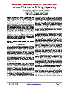
Figure 1: Brain tumor simulation results. The progression of the reaction-diffusion tumor model is shown. The leftmost image shows the initial condition; the rightmost image the solution of the forward problem at t = 1. The bottom row shows a 3D illustration and the top row an axial slice cut through the center of the tumor. White areas are locations of high tumor cell density and black areas locations of low density. The significance of our approach is threefold: automatic segmentation of patient images using normal subject images to create spatial (shape) priors; mapping of functional information from atlases to patients (critical in neurosurgery); and parameter calibration of biophysical models. Variants of algorithms similar to SIBIA that integrate biophysics with imaging (in low resolution) are already used in clinical settings [26, 51, 68]. In this paper, we focus on two subproblems: identifying initial conditions for a reaction-diffusion tumor growth model (inverse tumor parameter identification problem) and seeking a velocity that advects the atlas image to the patient image so that their L2 distance is small (image registration). Contributions. We introduce SIBIA, a framework that supports the solution of coupled image analysis and biophysical models. SIBIA provides solvers for various PDEs and their adjoints (for PDE constrained optimization), regularization operators, interfaces for medical images, and coupling between the different subproblems. The overall formulation follows closely several other approaches in biophysical modeling that opt for a simple but relatively versatile method using a pseudo-spectral fast Fourier-transform (FFT) for spatial differential operators and a semi-Lagrangian method for advection (to avoid time-step restriction). Our framework closely resembles our previous work in [47], where we introduced an algorithm for the image registration problem (only), described a semiLagrangian formulation, and discussed the use of FFTs and how to scale the overall methodology on distributed-memory architectures using the Message Passing Interface (MPI). In this paper, we follow the overall spirit of that formulation but with several novel contributions summarized below. Inverse tumor scalability: We scale the formulation for an inverse tumor growth problem described in [25] (MATLAB-based) and study its algorithmic and parallel scalability on real clinical data. A significant challenge is that the biophysical model involves PDEs with variable coefficients (due to spatiallyvarying tissue material properties). We discuss our preconditioner for the elliptic diffusion operator, and the inversion operator, the Hessian. Interpolation operator: The semi-Lagrangian advection requires interpolation from a regular grid to a grid of irregularly scattered points. In [47], we focused on the MPI implementation. As a result, the interpolation was a significant bottleneck consuming 60% to 75% of the runtime. Here we present an interpolation kernel that it is nearly 10× faster. It employs a reordering of points, blocking, and vectorization. We have ported our C++ implementation to

Intel Haswell architectures. Switching to single precision: Given the level of noise and imaging artifacts in the data, the modeling errors in the biophysical simulations, and the target levels of accuracy, double precision is not justified; we implement our solver in single-precision. This reduces the communication volume and the memory footprint for the adjoint solves (which require storing the time history). The work in [47] used one MPI task per socket (without OpenMP) and thus, in some sense, wasted resources. With SIBIA we can use 12 cores per node (for the largest runs) and 24 cores for the smallest runs with no problems. The two main computational kernels in SIBIA are FFT and interpolation. Our FFT is based on our open source library AccFFT [23, 24] but with a twist: we have implemented a faster field gradient computation, which halves the communication of the FFTbased PDE operators that we encounter frequently in our formulation. In §2, we discuss the different formulations. In §5, we present a detailed strong and weak scaling analysis for the tumor and registration solvers, the performance of the interpolation kernel, and comparisons with [47]. Another difference to [47], is that we use a more effective regularization functional [45]. Overall, SIBIA’s registration is 3 to 8 times faster than our previous work [47], supports stand-alone reaction-advection-diffusion solvers for biophysical inverse problems, and their coupling with registration. Limitations. SIBIA is limited to regular grids, like most software for MRI and CT images. If one needs non-uniform grids, other approaches are much more appropriate. Although the brain geometry is quite complicated, we use a penalty method to enforce boundary conditions. For image analysis, this is sufficient—given the large errors in the brain tumor model. Related work. To our knowledge, the most scalable deformable image registration algorithm is the one reported in [47]. For a detailed review on image registration algorithms see [47, 53, 59]. There are many scalable solvers for biophysical simulation but not much work for problems that are tightly coupled with MRI. In the latter area, most work is done on single node systems [12, 57]. For brain tumor applications, a good review of related work can be found in [5, 27]. The tumor model we are using is not predictive but it is quite standard in medical image analysis for tumors [34, 39, 48, 60, 61]. More sophisticated models [31, 36] have a large number of unknown parameters and are difficult to calibrate. Minimal models are preferable for medical image analysis [68].

A Framework for Scalable Biophysics-based Image Analysis


However, one important piece is missing in our model, the deformation of the brain parenchyma due to the tumor growth [34]. This is ongoing work. Regarding the numerical scheme for the tumor and registration, our formulation is motivated by the need for compatibility between imaging and biophysics and the need to accommodate different elliptic operators and fast solvers. We have to tackle three main elliptic-like operators: the diffusion step (with variable coefficients) for the tumor problem, the Hessian for the tumor inverse problem, and the Hessian for the registration inverse problem (Stokes-like operator). For these reasons we opted for an FFT-based solver due to its simplicity and robustness. Regarding fast FFT-based PDE solvers the literature is vast. For a review on parallel 3D FFT see [24].

2

MATHEMATICAL FORMULATION

We present the mathematical formulations for the considered problems next. We will see that both inverse problems are formulated as PDE constrained optimization problems. We use the method of Lagrange multipliers to solve them. We refer to [7, 9, 33] for excellent surveys on the theory and algorithmic developments in PDE constrained optimization. Data Assimilation in Brain Tumor Imaging. Our formulation for modeling the spatio-temporal spread of cancerous cells within brain parenchyma is widely adopted in the literature [1, 12, 25, 38, 48, 51, 60]. Our formulation captures the rate of change of cancerous cells represented as a population density c(x, t) based on two phenomena: proliferation and net migration of cells.1 The proliferation model is logistic, and the net migration of cancerous cells is modeled using an inhomogeneous (potentially anisotropic) diffusion operator (see below). This is the forward model, a non-linear parabolic PDE, for the tumor concentration2 c ∈ [0, 1] defined on the non-dimensionalized space-time interval Ω B × [0, 1]: ∂t c − ∇ · K∇c − ρc(1 − c) = 0 c = c0

in Ω B × (0, 1], in Ω B × {0}

(1a) (1b)

with homogeneous Neumann boundary conditions prescribed on ∂Ω B , where Ω B ⊂ Ω, Ω := [0, 2π )3 ⊂ R3 , is the spatial domain occupied by brain parenchyma and t ∈ [0, 1]. We remove all units from (1) by non-dimensionalization. We follow [25] and parameterize the initial condition c 0 (x) := c(x, t = 0) in an np -dimensional space spanned by a Gaussian basis, i.e., c 0 = Φp with the parameter vector p ∈ Rnp . The tensor K(x) ∈ R3×3 controls the net migration of cancerous cells c. The parameter ρ > 0 controls the proliferation. This simple reaction-diffusion model is by no means predictive on its own, but has been successfully used in conjuction with imaging information [26]. Its usefulness is in segmentation and registration algorithms that use normal atlas information, and in producing features (e.g., tumor parameters) to augment image-based features for tumor staging and prognosis. The inputs to our problem are probability maps of tissue types obtained from the patient’s imaging data [27, 50], in particular white matter πW (x), gray matter πG (x), cerebrospinal fluid πC (x), and πT (x). Figure 2 shows an exemplary dataset in the patient space.3 In 1 We note that this model is an approximation of the complex phenomena associated with cancer progression. More complicated models have appeared in the past [31]. Increasing the complexity of our model results in an excessive number of parameters (irrespective of the numerical strategy, optimize-then-discretize or discretize-thenoptimize), which have to be estimated from data or determined heuristically. 2 We interpret c as probability to encounter cancerous tissue at location x at time t . 3 This is a synthetic result based on a forward simulation on real brain imaging data.

πW

πG

πT

Figure 2: Illustration of the probability maps for different types of brain tissue. We display (from left to right) the probability maps for white matter πW (x), gray matter πG (x), and the tumor concentration πT (x) for an exemplary forward simulation. many existing approaches the probability maps πW (x) (white matter) and πG (x) (gray matter) control weights that enter K(x) with the common assumption that the cell diffusivity is larger in white matter than in gray matter [12, 38, 48, 60]. In our inverse tumor problem, we assume that we know K and ρ from experimental data; we only invert for the initial condition p. We consider isotropic diffusion, for which K(x) := (kW πW (x) + kG πG (x)) diag(1, 1, 1), parameterized by kW and kG . Given π j (x), j ∈ {T , C,W , G}, K, and ρ in the patient space, our task is to find the initial tumor density c 0 = Φp for (1) that best explains the tumor cell distribution πT (x) observed in the imaging data at t = 1; i.e., we seek to minimizes the L2 -distance between model output c 1 and patient observation πT . It is well known from inverse problem theory that the solution p is neither stable nor unique [29, 37]. One remedy is to stably compute the solution to a nearby problem by augmenting our formulation with a Tikhonov regularization model. The resulting inverse problem for recovering p (i.e., the initial condition c 0 ) from πT reads: ∫ γ 1 (c 1 − πT )2 dx + kΦp k22 dx p 2 Ω 2 B

min

(2)

subject to c 1 being given by the forward model in (1); γ > 0 balances regularity of p against the mismatch between c 1 and πT . To solve the inverse tumor problem, probability maps and parameters have to be given for the healthy brain without tumor. Because we do not have an estimate for the patient’s image without tumor, we use a standardized brain atlas template. To derive patient specific results, one approach is to couple image registration with the tumor problem [1, 27, 35, 69]. The main idea here is to use registration as a tool to minimize the differences between patient and atlas anatomies. We need to couple these processes, because a simple registration between the patient anatomy with tumor and the atlas anatomy is not possible due to ill-defined correspondences (i.e., presence of the tumor in only one image). We will address the coupling of our two approaches in future work. In the following section, we present the formulation for image registration. Diffeomorphic Image Registration. We refer to [20, 52, 59] for an introduction into the field of image registration and its applications. Image registration is a correspondence problem. The basic assumption is that there exists a geometric transformation that relates each point in one image, the so called reference image m R (x), to its corresponding point in another image, the so called template image mT (x). We illustrate this in Figure 3. We introduce a pseudo-time variable t ∈ [0, 1] and model this geometric transformation based on a transport equation for the intensity values of mT . The forward model of our problem is: Given a stationary velocity field v(x) and a template image mT (x) compute the transported intensities


A. Gholami et al.

m 1 (x) := m(x, t = 1) at t = 1 by solving in Ω × (0, 1], in Ω × {0},

(3a) (3b)

with periodic boundary conditions on ∂Ω forward in time. We again formulate the inverse problem as a PDE constrained optimization problem. The task is to find a plausible 4 velocity field v(x) so that the transported intensities of mT at t = 1 (i.e., the solution m 1 (x) := m(x, t = 1) of (3)) are similar to m R (x) for all x. Related formulations can, e.g., be found in [6, 8, 10, 30, 41, 44, 47, 64]. We search for a minimizer ∫ ∫ βv 1 min (m 1 − m R )2 dx + ∇v : ∇v dx (4) v 2 Ω 2 Ω subject to the forward model in (3). The second term in (4) enforces smoothness for v with the regularization parameter βv > 0 (where “:” denotes the matrix dot product5 ) . To be able to guarantee the existence and uniqueness of a solution of both, the forward and the optimization problem, one has to impose appropriate smoothness requirements on the images and the velocity.6 A key requirement in medical imaging is that the solution of (3) does not introduce any foldings, i.e., a volume element does not collapse to a single point, and characteristics traced by v do not cross. This is ensured by the regularization operator in (4). In this work, we additionally control the volume change by introducing a penalty on the divergence of v, i.e., we add the constraint ∇ · v = w and penalize variations in w by introducing an addition regularization norm with regularization weight βw > 0 [45]. Setting w to zero yields an incompressible diffeomorphism [10, 44, 47].7

3

ALGORITHMS

In this section, we discuss the discretization in space and time, the solvers, the computational kernels, and the parallel implementation of the optimization problems in §2. We use a globalized, preconditioned, inexact, reduced space Gauss–Newton method for both problems. Based on the derivation of the optimality conditions, we describe the individual numerical building blocks of our scheme. Optimality Conditions. We use the method of Lagrange multipliers [42] in an optimize-then-discretize approach. That is, we first compute variations of the Lagrangian functional with respect to the state, adjoint, and control variables, and then discretize them. We will see that the resulting equations are complex multi-physics operators that are challenging to solve in an efficient way. Tumor. The Langrangian function for the tumor reads ∫ ∫ γ 1 LT = (c 1 − πT )2 dx + kΦpk22dx + α 0 (c 0 − Φp) dx 2 ΩB 2 ΩB ∫ 1∫ + α (∂t c − ∇ · K∇c − ρc(1 − c)) dx dt (5) 0

ΩB

with the Langrange multiplier function α, and α 0 (x) = α(x, t = 0). We invert for the parametrization p for c 0 in (1a). The gradient of 4 The

notion of plausibility depends on the application (see, e.g., [53, 59]). We define a deformation map to be plausible if it is a diffeomorphism. 5A : B = Í i, j Ai j B i j . 6 We refer to [4, 6, 8, 10, 45, 64] for a theoretical discussion about uniqueness and well-posedness of the forward and inverse registration problem for our and related formulations. 7 The penalty on the divergence of v is controlled by controlling β . This allows us w to control the determinant of the deformation gradient (i.e., local volume change). This is different to the regularization parameter βv , which solely controls the smoothness of v . See [45] for more details.

дp := γ ΦT Φp − ΦT α 0

(6)

This defines the non-linear problem we have to solve for p. To obtain α 0 , we have to solve the adjoint equation stemming from the gradient of LT in terms of c: −∂t α − ∇ · K∇α − α ρ(1 − 2c) = 0 α − (πT − c) = 0

in Ω B × [0, 1), in Ω B × {1},

(7a) (7b)

with Neumann boundary conditions on ∂Ω B , backward in time. Note that the final condition in (7a) at t = 1 depends on c, which is the solution of the forward problem (1). Registration. The Lagrangian function of the image registration problem reads8 ∫ ∫ βv 1 LR = (m 1 − m R )2 dx + ∇v : ∇v dx 2 Ω 2 Ω ∫ 1∫ ∫ + λ (∂t m + v · ∇m) dx dt + λ 0 (m 0 − mT ) dx (8) 0

Ω

Ω

with the Lagrangian multiplier function λ and λ 0 (x) = λ(x, t = 0). We invert for the transformation velocity v. The gradient of LR in terms of v is given by ∫ 1 дv := −βv v + K[ λ∇m] dt, (9) ∇

∂t m + v · ∇m = 0 m = mT

LT in terms of p is given by

0

where K is a pseudo-differential operator that enforces additional constraints on the divergence of v (see [45]; for (8), K is simply an identity operator). To evaluate дv in (9) for a candidate velocity field v, we need to find the state and adjoint variable m(x, t) and λ(x, t), respectively. We obtain them from setting the gradients of LR in terms of λ and m to zero, i.e., by solving (3a) forward in time and using m at t = 1 as an initial condition for the adjoint equation: −∂t λ − ∇ · λv = 0 λ = mR − m

in Ω × [0, 1), in Ω × {1}

(10a) (10b)

with periodic boundary conditions on ∂Ω, backward in time. Having found λ(x, t), we can evaluate (9). In our actual implementation, we do not store λ. We integrate the second term in (9) directly when solving (10), instead. This allows us to make the memory requirements of our solver almost independent of nt ; we only have to store the transported intensities m (to be able to evaluate the Hessian matvec). Finally we remark that both problems are nonconvex, and our methods target a local minimum. Spatial Discretization. We use regular grids to discretize the space-time interval Ω × [0, 1], Ω := [0, 2π )3 ⊂ R3 . The spatial grid consists of N 0 × N 1 × N 2 , Ni ∈ N grid points xi := (x 0,i , x 1,i , x 2,i ) ∈ R3 , x j,i := 2πi j /N j , 0 ≤ i j ≤ N j − 1, j = 0, 1, 2. We follow [47] and use a spectral projection scheme for all spatial operations. Our formulations (including images) are periodic and continuously differentiable. We apply appropriate filtering operations and periodically extend or mollify the discrete data to meet these requirements. The tumor problem in (1) requires Neumann boundary conditions on the surface of the brain ∂Ω B . We follow [25, 35] and use a penalty approach to approximate these boundary conditions. We apply periodic boundary conditions on ∂Ω and set the diffusion coefficient outside of Ω B equal to a small penalty parameter K ϵ . 8 We

neglect the incompressibility constraint for clarity.



before

after

reference image template image deformed template image residual differences Figure 3: Image registration. The inputs to this inverse problem are scalar intensity values of two images of the same object (left). The deformed template image is illustrated in the middle. The residual between the images before and after registration is shown on the right. The images depicted here are a 2D illustration (axial slice) of the 3D image registration problem solved in §5. Numerical Time Integration. Fulfilling the first order optimality conditions, i.e., zero gradients of the Lagrange formulation, requires a repeated solution of parabolic or hyperbolic PDEs. In the following, we sketch our time integration schemes for these systems. Parabolic PDEs. We follow [25, 35] and use an unconditionally stable, second-order Strang-splitting method to solve the parabolic equations (1) and (7). We explain this for the forward problem (1). Let cj ∈ RN denote the tumor distribution at time t j = j∆t, ∆t = 1/nt . We apply an implicit Crank–Nicolson method for diffusion and solve the reaction part analytically: (I − 0.25∆tD)c† = (I + 0.25∆tD)cj

(11)

scheme. Note that, since we invert for a stationary velocity field v(x), (15) needs to be solved only once during each Newton step. Inversion. We use a matrix-free, globalized, inexact Gauss–Newton algorithm for numerical optimization. The update rule for a control variable uk at iteration k reads uk +1 = uk − α k H−1 g, α k > 0, (18) −1 where H is a Gauss–Newton approximation of the inverse of the Hessian9 , g a discrete representation of the gradient of the optimization problem. For the tumor case, the control variable uk is given by p ∈ Rnp and for the registration by v ∈ R3n with N = N 0 N 1 N 2 . The step length α k > 0 is determined by an Armijo line search and is chosen such that we decrease the value of the objective function in every iteration. Storing and inverting H using a direct solver is prohibitively expensive. We use an iterative PCG method instead, which only requires an expression for the action of the Hessian on a vector (Hessian matvec). We further reduce computational cost by inverting H only inexactly [17, 55]. Our solver uses PETSc’s TAO module [3, 54]. Our code implements the operations for evaluating the objective functions, the gradient, and the Hessian matvec. Despite the complexity of the whole formulation, it turns out the main computational bottlenecks are FFTs and interpolations. We will see in §5 that these computations make up 80% to 90% of the entire time spent in the solver. We will describe the parallel implementation of these kernels and present dedicated strategies to significantly speed up their single core performance next.

e image deformed template image j

∂t c = ρc(1 − c) j

c(t ) = c

(I − 0.25∆tD)c

j+1

in (t , t

j+1

†

)

(12) (13)

= (I + 0.25∆tD)c(t

j+1

).

(14)

We use a PCG method with a fixed tolerance of 1e−6 to solve (11) and (14). The preconditioner is based on a constant coefficient ap˜ = I − 0.25∆t K˜ , where K˜ > 0 is the proximation of D given by D average diffusion coefficient. The inversion and construction of this preconditioner has vanishing computational cost due to our spectral scheme; it only requires one Hadamard product in the frequency domain and one forward and backward FFT. This preconditioner can be shown to result in a mesh independent condition number as long as the mesh is fine enough to resolve the diffusion coefficient. Since, for medical images, we can have large contrast and sharp transitions, the grid to resolve the operator can become prohibitively large; a lack in resolution manifests in an increase in the number of Krylov iterations, as we increase the mesh size. ∇

Hyperbolic PDEs (Transport Equations). We employ a semiLagrangian scheme [18] to solve the hyperbolic transport equations. The use of semi-Lagrangian schemes in the context of image registration is not new; see [6, 10, 46, 47] for details. Semi-Lagrangian schemes are unconditionally stable, which allows us to keep the number of time-steps small. This is critical for large-scale 3D applications. The solution algorithm for one time step of a transport equation (3), e.g., consists of two steps: backward in [t j , t j+1 )

solve dt y = v(y) y(t m(x, t

j+1 j+1

)=x

(15) (16)

j

j

) = m(y(t ), t ).

(17)

The scheme requires evaluating v and m along y, i.e., at locations that do not coincide with grid points. Both steps involve interpolation. It is critical to design a fast interpolation operator (see §4). Our ODE solver for (15) is a second-order explicit Runge–Kutta

4

PARALLEL ALGORITHMS AND COMPUTATIONAL KERNELS

The main computational kernels of SIBIA are the FFT used for spatial differential operators in our spectral approach and the interpolations in the semi-Lagrangian scheme for advection. Below, we discuss specific performance optimizations for each of these two. FFT for Spectral Operators. Spatial differential operators such as gradient or divergence can be computed in our spectral approach by first transforming the input field into the frequency domain (FFT), followed by a Hadamard transform and an inverse FFT. We use a 2D pencil decomposition for 3D FFTs [16, 28] to distribute the data among processors and support parallel FFT on CPU/GPU for both single and double precision computations. Exemplarily, we consider computing the x derivative of a scalar field f : f x = Fx−1 (−iωx Fx (f )), (19) where Fx denotes the FFT transform in x direction. Note that, to compute the x derivative, we only need a batched 1D FFT instead 9 We

can derive the Hessian from the second variations of the Lagrangian functional of our problem. We omit these details and refer to related work [2, 25, 44, 45, 47].


A. Gholami et al.

Table 1: Experiment to evaluate the efficiency of the binning method in the interpolation. We use N fixed departure coordinates and compare the results with those for random departure coordinates within each processor’s domain. In the random test, different grid values have to be loaded per departure point, but in the fixed point test they are loaded only once. The first two columns show the total interpolation time and GFLOPS for the fixed test. The rest of the columns show the resutls for the random points experiemnt for with/without binning and vectorization. For large problem sizes, the main speedup is achieved by the binning. The experiment was performed on 1 Haswell node with 24 MPI tasks. The reported GFlops include the time needed to reshuffle the interpolated values in the binning method. Fixed Point N 643 1283 2563 5123

Interp Time 1.8e−4 1.4e−3 1.4e−2 1.1e−1

GF 356 347 287 287

No Bin, No SIMD Interp Time GF 1.4e−3 45 1.2e−2 42 1.5e−1 28 2.6 13

Random Departure Points Bin, No SIMD No Bin + SIMD Interp Time GF Interp Time GF 1.4e−3 45 2.2e−4 280 1.1e−2 44 3.4e−3 146 8.8e−2 45 3.4e−3 54 8.1e−1 40 1.7 19

Algorithm 1: Fast algorithm for computing x derivative, which only requires two global transposes as opposed to four. Input : Data in spatial domain. Layout: N 0 /P 0 × N 1 /P 1 × N 2 Output : x derivative b0 /P0 × N 1 /P1 × N 2 Layout: N T

N 0 × N 1 /P0 × N 2 /P1 ←−−−− N 0 /P 0 × N 1 /P 1 × N 2 ; // input data F FT b0 × N 1 /P0 × N 2 /P 1 ← N −−−− N 0 × N 1 /P0 × N 2 /P1 ; // Hadamard and T b b0 × N 1 /P0 × N 2 /P1 ; // x derivative N 0 /P 0 × N 1 × N 2 /P 1 ←−−− N

FFT

of a 3D FFT. This saves a large amount of communication since no repartitioning of data for the pencil decompositions in y direction is required. However, we still have to perform a global transpose to establish the pencil decomposition in x direction. This is followed by a forward FFT transform in x direction, a Hadamard product, a local inverse FFT, and another global transpose to redistribute the data. Parallel FFT libraries such as P3DFFT or AccFFT allow the user to specify which directions the local forward/inverse FFT is needed but there is no way to avoid unnecessary global transposes in y direction (or x when computing y derivative). We have enhanced AccFFT such that it avoids all unnecessary global transposes, which for the x derivative reduces 4 global transposes to just 2 (as shown in Algorithm 1). This new implementation reduces the total global transposes to 4 for the gradient (as opposed to 8), and 4 for the divergence operator (as opposed to 8) 10 . This reduces the communication volume by a factor of two. Interpolation. As explained in §3, the transport equations in the registration are solved using Semi-Lagrangian scheme that requires costly interpolation of velocities and image data along backward characteristics. The value of a scalar (or vector) field f , at an off-grid point (x, y, z) (departure coordinate) can be computed as: f (x, y, z) =

d Õ d Õ d Õ i=0 j=0 k =0

li (x) =

d Ö

fi jk `i (x)`j (y)`k (z),

x − xn , x − xn n=0;i,n i

(20) (21)

Bin + SIMD Interp Time GF 2.1e−4 295 2.0e−3 256 2.3e−2 173 2.9e−1 112

Speedup 6.56 x 6.1 x 6.18 x 8.62 x

registration quality. Therefore, we focus on optimizing cubic order interpolation, which requires the computation of 12 Lagrange basis polynomials and the evaluation of Eq. 20 for each departure point. Note that each departure point requires a different set of 64 fi jk grid values, which creates a significant number of cache misses that cannot be hidden by the few floating point computations. However, it is possible to alleviate this problem by a novel approach: There is no reason to process the departure points based on the order that they were received. Instead, we can group the departure coordinates that are close to each other. We achieve this by sorting the departure points during the scatter phase using morton sort (which is a space filling sort). We optimized this sorting by partitioning the domain and the departure points into bins, i.e., patches of 16×16×16 grid cells. Instead of sorting all departure points, we just sort the bin ids to determine offline which bin has to be processed first. This phase can actually be performed offline analytically since it does not depend on the departure point coordinates (only depends on the grid and bin size). Our experimental results show that this approach is very effective in reducing cache misses. In addition, we use SIMD vectorization for the interpolation kernel (based on AVX2 on Haswell). The effect of each of these optimization is tested on Lonestar5, results are presented in Table 1. The second focus for optimization in parallel interpolation is the scatter phase, i.e., sending all points on the backward characteristics that land in another processor’s domain to the respective MPI rank. These communications are costly and affect the scaling. However, since the velocity field is stationary, we need to only scatter the coordinates of the off-grid interpolation points once for each advection problem. We use a sparse point-to-point alltoallv for communicating these data. In summary, our optimizations for the interpolation kernel include a novel approach to reduce cache misses by using a binning method, AVX vectorization of the kernel, and OpenMP support resulting in a significantly better interpolation kernel than the one presented in the work of [45]. We are now bound by the communication time instead of the time spent in interpolation kernel.

5

RESULTS

where fi is the function value at grid point i, `i is the i th Lagrange basis polynomial, and d is the interpolation order, which is cubic in our algorithm. Using a higher order method would lead to better hardware performance, but in practical applications with real data, the use of higher order interpolation does not improve the

We report results for the tumor inversion and for the registration. We report the overall runtime,11 execution and communication times for the computational kernels, and the total time spent to evaluate these kernels.12 We always report the maximum time across all MPI tasks. We will also discuss the algorithmic scalability of the tumor diffusion solver, i.e., the number of PCG iterations as we

10 Note

11 The runtime is the time spent on the entire inversion (excluding setup and I/O times).

that we do not need 8 global transposes since the z direction is owned locally by each process, and we only need to perform local FFTs to compute the gradient in z direction.

12 The overall kernel evaluation time includes execution, communication, and shuffling

of the data.

A Framework for Scalable Biophysics-based Image Analysis increase the problem size. We also discuss parallel scalability of the different kernels, and report the overall scalability. Setup, Implementation, and Hardware. We execute runs on Lonestar 5 (2-socket Xeon E5-2690 v3 (Haswell) with 12 cores/socket, 64 GB memory per node) and Hazel Hen (same node as Lonestar but with 128 GB memory per node). Our code is written in C++ and uses MPI for parallelism. It is compiled with the default Intel compilers available on the systems (Intel 16). We use PETSc’s implementations for linear algebra operations and PETC’s TAO package for the nonlinear optimization [3, 54], AccFFT for Fourier transforms [23, 25], and PnetCDF for I/O [63]. Data assimilation in brain tumor imaging. In this section, we study the computational performance and parallel scalability of the tumor inversion solver for real brain data as illustrated in Figure 1. We use resampled medical brain image data with a spatial resolution N ∈ {643 , 1283 , 2563 , 5123 } and present scalability results for up to 16, 384 MPI tasks on Hazel Hen. Setup. For all tumor inversion experiments, we set the regularization parameter γ = 10−3 , the number of time steps nt = 4 and use double precision. We perform three Gauss-Newton iterations for the inversion and limit the number of Hessian matvecs in the PCG solver to three. This setup results in an overall gradient reduction by one order of magnitude and 13% relative mismatch for the reconstructed tumor. Using nt = 4 is not sufficient to resolve the dynamics accurately but it puts pressure on the forward solver and allows us to monitor its algorithmic scalability. We report the time to solution as well as the percentage and absolute time spent in the Hessian matvec, the PCG solver and the FFT, which is the main computational kernel in the tumor inversion. For all the strong scaling runs, we use 12 MPI tasks per node. Strong Scaling. We report scaling results for different spatial resolutions N ∈ {643 , 1283 , 2563 , 5123 } and different numbers of MPI tasks P ∈ {21 , . . . , 214 }. The results are reported in Table 2. For N = 2563 , we observe excellent strong scaling performance with a parallel efficiency of 98 %, going from 32 to 2048 MPI tasks (runs #13– #19). The time consumed by the FFT accumulates to approximately 82 % of the overall runtime. Thus, the tumor inversion scalability is mainly inherited from the AccFFT. Similar conclusions can be drawn from the N = 1283 and N = 643 experiments, yielding a slightly lower but still acceptable parallel efficiency of 67 % from 4 to 256 MPI tasks and 52 % from 2 to 32 MPI tasks, respectively The ideal runtime (assuming 100% parallel efficiency) along with the actual runtime and the amount of time spent in the FFT are summarized in Figure 4 for the strong scaling experiments given in Table 2. Considering the N = 5123 runs, we observe a degradation of the parallel scalability for more than 2048 MPI tasks (runs #24– #27). Our analysis showed that MPI routines generate an increasing overhead using more than 2048 MPI tasks with 12 tasks per node. Increasing the MPI buffer size and the maximum message size for the MPI eager messaging protocol improved the performance of run #25 by around 30 % (run #26). Usually, the diffusion solve consumes up to 98 % of the overall runtime, which, drops down to 50 % for the runs that show poor scalability, indicating that performance is lost due to non-optimized MPI settings. Summarizing, for up to a total number of 2048 MPI tasks, we get almost optimal strong scaling results with a parallel efficiency from 60 % up to 100 %, cf. Figure 4. We encounter some MPI related communication issues going beyond 2048 MPI tasks. Using hybrid parallelism with OpenMP is expected to resolve the issue.

SC17, November 12–17, 2017, Denver, CO, USA Weak Scaling. For the same setting, we analyze algorithmic and fW , respectively, in parallel weak scaling, indicated by effW and eff Table 2 (exemplarily highlighted, runs #3, #10, #17, #24, #26). We observe an algorithmic weak scaling efficiency of around 30 %, increasing both, the number of unknowns in space and the number of MPI tasks by a factor of eight. Since the grid is not sufficiently large to resolve the diffusion operator, we observe a mesh-dependent number of iterations with increasing resolution—from 10 iterations per diffusion solve (on average) for N = 643 to 50 per diffusion fW , solve for N = 10243 . For the parallel weak scaling efficiency eff where we keep the number of PCG iterations constant yielding an efficiency of about 45 %, again increasing the number of unknowns and the number of tasks by a factor of eight. With respect parallel efficiency, the weak scaling performance perfectly correlates with the FFT, which in turn deteriorates due to the communication. Using only two MPI tasks per node (one per socket), the (parallel) weak scaling efficiency increases to 80 % going from resolution 643 to 1283 (runs #29–#32), which is acceptable considering the overhead for memory allocation and increasing communication time. We solve the inverse tumor problem for realistic brain geometries with a 2563 resolution up to a relative gradient of 1.20e−4 in 22 minutes using 512 MPI tasks on Hazel Hen. This corresponds to a reduction of the objective function by three orders of magnitude and a relative reconstruction mismatch of 0.2 %. Diffeomorphic registration. We consider an open-access data repository that has been widely used in the medical image computing community to study the performance of diffeomorphic image registration algorithms—the Non-rigid Registration Evaluation Project (NIREP) [11]. This data is illustrated in Figure 3. The original resolution of the data is (N 0 , N 1 , N 2 ) = (256, 300, 256).13 We also consider a simple test example to demonstrate large-scale results for grid sizes of up to 40963 . This results in an inversion for ∼ 200 billion unknowns (if we just count the velocity field v and ignore the state and adjoint fields). This synthetic problem (SYN) is generated by solving the forward problem. We set the template image to mT (x) = (sin(x 1 )2 + sin(x 2 )2 + sin(x 3 )2 ))/3 and transport it with the velocity velocity v(x) = (v 1 (x), v 2 (x), v 3 (x), v 1 (x) = sin(x 3 ) cos(x 2 ) sin(x 2 ), v 2 (x) = sin(x 3 ) cos(x 3 ) sin(x 3 ), and v 3 (x) = sin(x 2 ) cos(x 1 ) sin(x 1 ). Setup. We fix several parameters across all runs: We use twelve MPI tasks per node. We set the number of time steps to nt = 4. We use an H 1 regularization model with a penalty on the divergence of v to control volume change (regularization weight βw = 1e−4). We use a quadratic forcing sequence. We report a strong scaling analysis using the NIREP datasets with resolution levels κl · (256, 300, 256), κl ∈ {1/4, 1/2, 1, 2}. We empirically set the regularization parameter for the velocity v to βv = 1e−2. We limit the number of Newton iterations to three and the number of PCG iterations to five. The relative tolerance for the gradient is set to 1e−1 (we do not reach this tolerance for these runs). We limit the Newton iterations to five and the Krylov iterations to ten for the synthetic large scale runs (N = 10243 , N = 20483 , and N = 40963 ). The relative tolerance for the gradient is 1e−2. We also report a run for the entire inversion. We set the relative tolerance for the gradient to 1e−1. This run is performed on the same images we used in [45]. Results. We report the strong scaling analysis for the NIREP datasets as well as the synthetic large scale run in Table 3. We illustrate the 13 We

transfer the images to a finer or coarser grid based on a cubic interpolation model. We band-limit the data by applying a Gaussian smoothing operator with a spatial bandwidth of h i , i = 1, 2, 3.


A. Gholami et al.

Table 2: Computational performance of the tumor solver for real brain data, illustrated in 1 on HLRS’s Hazel Hen. We perform three Gauss-Newton iterations with a regularization parameter γ = 10−3 , and limit the number of Hessian matvecs in the PCG solver to a maximum of three. We report time to solution, time spent in the Hessian matvec, in the FFT, and in the diffusion solver, respectively (in seconds). We show the strong scaling e , the number of PCG iterations for efficiency effS and the algorithmic weak scaling efficiency effW . For the parallel weak scaling efficiency eff W the diffusion solver is fixed for all spatial resolutions. Timings are reported as a function of the number of unknowns (in space), and the number of nodes and tasks. For runs marked with † we encountered MPI problems due to non-optimal settings. Performance could be improved by increasing the MPI buffer and the maximum message size for the MPI eager protocol (run marked ‡). N

nodes

tasks

runtime

effS

effW

fW ) (eff

FFT

([%])

H-matvec

([%])

diffusion

([%])

#1 #2 #3 #4 #5

643

1 1 1 2 3

2 4 8 16 32

4.07e+1 2.60e+1 1.33e+1 6.05 4.81

100.0 78.2 76.6 84.0 52.8

100.0 100.0 100.0 100.0 100.0

(100.0) (100.0) (100.0) (100.0) (100.0)

3.23e+1 2.12e+1 9.92 5.05 4.14

(79.5) (81.7) (74.7) (83.5) (86.1)

2.57e+1 1.64e+1 8.38 3.82 3.02

(63.2) (63.3) (63.1) (63.2) (62.8)

3.98e+1 2.55e+1 1.30e+1 5.89 4.68

(97.8) (98.1) (97.9) (97.4) (97.3)

#6 #7 #8 #9 #10 #11 #12

1283

1 1 2 2 6 11 22

4 8 16 32 64 128 256

4.91e+2 3.07e+2 1.37e+2 8.46e+1 4.15e+1 2.08e+1 1.13e+1

100.0 80.0 89.6 72.6 73.9 73.7 67.7

(43.7) (45.2) (46.8) (42.0) (60.9)

4.24e+2 2.56e+2 1.12e+2 6.72e+1 3.24e+1 1.71e+1 9.49

(86.3) (83.2) (81.5) (79.5) (78.1) (82.2) (83.7)

3.14e+2 1.96e+2 8.77e+1 5.41e+1 2.65e+1 1.33e+1 7.20

(63.9) (63.9) (64.0) (63.9) (63.9) (63.8) (63.5)

4.87e+2 3.04e+2 1.36e+2 8.38e+1 4.11e+1 2.06e+1 1.11e+1

(99.2) (99.1) (99.2) (99.1) (99.0) (98.7) (98.0)

#13 #14 #15 #16 #17 #18 #19

2563

3 6 11 22 43 86 172

32 64 128 256 512 1024 2048

1.58e+3 8.06e+2 3.63e+2 1.81e+2 1.00e+2 4.03e+1 2.50e+1

100.0 98.2 109.0 109.6 98.9 123.0 98.9

(22.9) (29.3) (26.6) (31.0) (38.5)

1.31e+3 6.75e+2 3.01e+2 1.49e+2 8.26e+1 3.45e+1 2.17e+1

(82.9) (83.7) (82.9) (82.6) (82.5) (85.7) (86.9)

1.02e+3 5.19e+2 2.35e+2 1.16e+2 6.45e+1 2.55e+1 1.59e+1

(64.4) (64.4) (64.7) (64.4) (64.4) (63.4) (63.5)

1.57e+3 7.99e+2 3.61e+2 1.80e+2 9.95e+1 3.97e+1 2.38e+1

(99.1) (99.1) (99.5) (99.5) (99.3) (98.6) (95.0)

#20 #21 #22 #23 #24 #25† #26‡ #27†

5123

22 43 86 172 342 683 683 1366

256 512 1024 2048 4096 8192 8192 16384

2.52e+3 1.32e+3 7.54e+2 3.47e+2 2.57e+2 2.00e+2 1.43e+2 3.89e+2

100.0 95.8 83.5 90.7 61.2 39.3 55.1 10.1

5.4 7.5 5.2 3.0 4.2 1.2

(13.6) (19.0) (11.6) (5.6) (7.8) (2.0)

2.15e+3 1.13e+3 6.24e+2 2.87e+2 1.98e+2 1.30e+2 9.20e+1 2.16e+2

(85.2) (86.2) (82.8) (82.8) (77.1) (65.1) (64.4) (55.6)

1.65e+3 8.61e+2 4.93e+2 2.32e+2 1.66e+2 1.32e+2 8.96e+1 2.34e+2

(65.5) (65.5) (65.4) (66.9) (64.6) (65.9) (62.7) (60.2)

2.50e+3 1.31e+3 7.52e+2 3.45e+2 2.50e+2 1.71e+2 1.15e+2 2.69e+2

(99.4) (99.4) (99.7) (99.4) (97.3) (85.5) (80.7) (69.2)

#28

10243

2732

32768

1.61e+3

100.0

0.8

(1.2)

6.58e+2

(40.9)

9.25e+2

(57.5)

8.19e+2

(50.8)

#29 #30 #31 #32

643 1283 2563 5123

2 16 128 1024

4 32 256 2048

2.20e+1 4.00e+1 6.96e+1 1.39e+2

100.0 55.0 31.6 15.9

(100.0) (80.7) (64.8) (37.5)

1.85e+1 3.49e+1 6.05e+1 1.14e+2

(84.2) (87.2) (87.0) (82.3)

1.40e+1 2.56e+1 4.52e+1 8.82e+1

(63.5) (64.1) (65.0) (63.7)

2.15e+1 3.94e+1 6.90e+1 1.36e+2

(97.7) (98.6) (99.1) (98.2)

29.7 30.7 32.0 29.0 42.5

11.2 14.4 13.3 15.0 19.2

Figure 4: Summary of strong scaling efficiency of tumor inversion for real data. See Table 2 for exact timings. We display time to solution and time spent in the FFT (in seconds) as a function of the number of unknowns (in space) and the number of tasks.



#22 #23 #24 #25 #26 #27 #28

eff.

total FFT

([%])

FFT comm.

total interp.

([%])

interp. kernel

interp. comm.

(64, 75, 64)

#13 #14 #15 #16 #17 #18 #19 #20 #21

runtime

1 1 1 2 3

2 4 8 16 32

2.07 1.13 6.26e−1 3.70e−1 2.47e−1

100.0 91.4 82.6 69.9 52.3

8.21e−1 4.83e−1 2.67e−1 1.72e−1 1.27e−1

(39.7) (42.7) (42.7) (46.6) (51.3)

9.31e−2 7.36e−2 4.44e−2 6.88e−2 7.51e−2

1.05 5.30e−1 2.87e−1 1.59e−1 9.28e−2

(51.0) (46.8) (45.9) (43.1) (37.5)

7.18e−1 3.70e−1 1.95e−1 9.84e−2 5.00e−2

6.71e−2 3.68e−2 1.78e−2 9.95e−3 5.54e−3

(128, 150, 128)

#6 #7 #8 #9 #10 #11 #12

tasks

1 1 1 2 3 6 11

2 4 8 16 32 64 128

2.15e+1 1.13e+1 6.19 3.30 1.79 1.04 6.49e−1

100.0 95.4 86.9 81.6 75.2 65.0 51.8

9.35 5.06 2.79 1.59 8.94e−1 5.61e−1 3.69e−1

(43.4) (44.9) (45.0) (48.2) (50.0) (54.2) (56.9)

5.07e−1 6.73e−1 3.89e−1 5.52e−1 3.86e−1 3.68e−1 2.64e−1

9.91 5.05 2.78 1.44 7.50e−1 4.22e−1 2.47e−1

(46.0) (44.7) (44.9) (43.6) (41.9) (40.8) (38.1)

6.83 3.42 1.82 9.24e−1 4.63e−1 2.32e−1 1.22e−1

8.22e−1 4.28e−1 2.32e−1 1.14e−1 5.93e−2 3.05e−2 1.90e−2

(256, 300, 256)

N #1 #2 #3 #4 #5

nodes

1 1 1 2 3 6 11 22 43

2 4 8 16 32 64 128 256 512

2.36e+2 1.22e+2 6.73e+1 3.59e+1 1.81e+1 9.70 4.63 2.66 1.52

100.0 96.4 87.6 82.1 81.4 76.0 79.5 69.2 60.5

1.13e+2 6.04e+1 3.23e+1 1.82e+1 9.38 5.57 2.72 1.63 8.09e−1

(48.0) (49.3) (48.0) (50.7) (51.8) (57.5) (58.6) (61.1) (53.1)

6.40 8.33 4.58 7.80 3.60 3.30 1.50 1.21 6.15e−1

1.02e+2 5.25e+1 2.99e+1 1.55e+1 7.48 3.93 1.69 9.81e−1 6.43e−1

(43.4) (42.9) (44.5) (43.2) (41.3) (40.5) (36.5) (36.9) (42.2)

5.88e+1 2.95e+1 1.56e+1 7.82 3.92 1.99 9.98e−1 4.98e−1 2.54e−1

1.05e+1 5.51 3.95 2.69 1.18 7.07e−1 1.49e−1 8.26e−2 6.80e−2

(512, 600, 512)

Table 3: Image registration scaling performed on TACC’s Lonestar 5 (runs #1 to #28; NIREP datasets; see Figure 3) and HLRS’ Hazel Hen (SYN datasets). We use 12 MPI tasks per node. We set the upper limit for the Gauss–Newton iterations to three/five and the number of PCG iterations to five/ten for NIREP/SYN. We report (from left to right) the total time spent in the inversion (runtime/time-to-solution), the strong scaling efficiency, and the time spent in the computational kernels (spectral operations/FFT and interpolation), respectively (in seconds) as a function of the number of unknowns N (in space), and the number of nodes and tasks. Here “total FFT” corresponds to the time spent in all spectral operations; “FFT comm.” is the communication time; “total interp.” is the overall time spent in the interpolation; “interp. kernel” is the time spent on the execution of the interpolation operator, and “interp. comm” is the communication time for the interpolation. We also report the strong scaling efficiency and the percentage of the total interpolation and FFT time with respect the overall runtime.

2 3 6 11 22 43 86

16 32 64 128 256 512 1024

3.28e+2 1.73e+2 8.66e+1 4.32e+1 2.36e+1 1.31e+1 6.35

100.0 94.7 94.7 94.9 87.0 78.1 80.7

1.81e+2 9.57e+1 5.04e+1 2.46e+1 1.56e+1 8.92 4.35

(55.0) (55.2) (58.2) (56.9) (66.3) (67.9) (68.5)

4.84e+1 2.85e+1 2.42e+1 1.10e+1 1.08e+1 6.56 3.52

1.35e+2 6.86e+1 3.48e+1 1.63e+1 8.83 4.41 2.02

(41.2) (39.6) (40.2) (37.8) (37.5) (33.6) (31.9)

6.33e+1 3.17e+1 1.59e+1 7.95 4.03 2.03 1.02

2.50e+1 1.15e+1 6.31 2.84 1.64 7.27e−1 2.08e−1

#29 #30

10243

11 22

128 256

1.97e+2 9.88e+1

100.0 99.7

1.20e+2 6.17e+1

(60.9) (62.5)

3.30e+1 2.15e+1

6.90e+1 3.49e+1

(35.0) (35.4)

2.35e+1 1.16e+1

2.23e+1 1.16e+1

#31 #32

20483

86 171

1024 2048

2.10e+2 1.11e+2

100.0 94.8

1.37e+2 7.17e+1

(65.0) (64.7)

4.33e+1 2.63e+1

7.21e+1 3.64e+1

(34.3) (32.8)

2.73e+1 1.35e+1

2.40e+1 1.05e+1

#33 #34

40963

342 684

4096 8192

4.42e+2 2.38e+2

100.0 93.1

3.22e+2 1.73e+2

(72.8) (72.9)

1.31e+2 8.27e+1

1.17e+2 6.25e+1

(26.4) (26.3)

4.20e+1 2.10e+1

3.97e+1 2.30e+1

strong scaling results for the real data also in Figure 5. We report accumulated timings for the max values across all MPI tasks in seconds as well as the strong scaling efficiency. The timings are as follows: (i) “total FFT”: time spent in all spectral operations; (ii) “FFT comm.” communication time for the FFT, (iii) “total interp.”: overall time spent in the interpolation, (iv) “interp. kernel”: time spent on the execution of the interpolation operator, and (iv) “interp. comm”: communication time for the interpolation. We also report the percentage of the total interpolation and FFT time with respect to the overall runtime. Observations. We spend almost all time (∼90%) in the execution of the FFT and the interpolation (see Table 3 and Figure 5). We achieve excellent strong scaling results for clinically relevant problem sizes, with an almost perfect scaling for the execution of our

computational kernels (application of the FFT and evaluation of the interpolation operator locally). We can fit conically relevant problems on one a single node with 64GB of memory (see, e.g., run #13). The number of MPI tasks for a specific problem size is, in our current implementation, limited by the support of the interpolation kernel/the size of the ghost layer; for a cubic interpolation model, we need at least 3 × 3 × N 2 points on each MPI task. We showcase results that demonstrate that our solver can be used to solve registration problems of unprecedented scale (40963 resulting in ∼ 200 billion unknowns—a problem size that is 64× bigger than the state-of-the-art that we presented at SC16 [45]. The weak scaling efficiency for these runs is 62.7%, 44.6%, and 32.6% when comparing the runtime for run #1 to the runs #9, #19, through #28. The communication time for the FFT increases as we


A. Gholami et al.

Figure 5: Strong scaling performance for diffeomorphic image registration. The results correspond to Table 3. We report the time to solution and the time spent in the computational kernels (summarized), respectively (in sec.) as a function of the number of unknowns (in space), and the number of MPI tasks. increase the problem size. We expect to see this behavior, since the FFT is communication bound. This negatively affects our weak scaling results (the total FFT time is for run #28 almost exclusively dominated by the FFT communication time; 80%). This observation is consistent with the results we report for the tumor case. The weak scaling performance for the interpolation is very good (50% in total when comparing runs #1 and #28). Having good strong scaling performance is important in image registration, as the time to solution can be prohibitive in 3D. We can see that we achieve a quite good strong scaling for our runs (between 52.1% (run #5) and 80% (run #28); this is in particular visible in Figure 5. The execution times for our computational kernels show excellent strong scaling results. The efficiency eventually deteriorates as we increase the number of cores. The amount of data we have to communicate in the interpolation phase essentially depends complexity of the characteristic. In a worst case scenario (which we do not expect in practical applications) all departure points may end up on one node. Semi-Lagrangian schemes can help us to alleviate potential imbalances (in contrast to purely Lagrangian schemes [6]). If the characteristic becomes to complex, we can introduce more time points to our problem. However, this will negatively affect the time-to-solution, as we have to perform more interpolations.14 We analyze our results for original resolution of the NIREP data sets in more detail: For these experiments, we can reduce the gradient by a factor of 3.17e−1 and the mismatch between the transported template image and the reference image by a factor of 1.89e−115 . The balance of the runtime spent on the individual components of our scheme is the same throughout all runs. We perform 32 PDE solves. The PDE solves is where the entire runtime goes. For instance, for run #13 we spend 87% of the total runtime (2.36e+2 sec. of 2.06e+2 sec.) on solving the transport equations of our system. These solves are done in the evaluations of (i) the objective functional (four evaluations.; 1.85e+1 sec.), the gradient (four evaluations.; 2.69e+1 sec.), and the Hessian matvec (twelve evaluations.; 1.78e+2 sec.). As we can see from this analysis, we spend most of the time runtime on the Hessian matvec. When we switch from two MPI tasks to 512 we can reduce the run time by a factor of about 150 (1.52 sec.; 60.5% efficiency). For the synthetic case we can solve our problem (reduce the gradient by two orders of magnitude) within 14 An

analysis of the number of interpolations we have to perform can be found in §3. that we discussed convergence rates for further mismatch reduction in [46] such that we focus on weak/strong scaling for different images and less for convergence rates, here. The tolerances and mismatch values chosen here allow for comparison of timings that we reported in [47]. Thus, we limited the number of Newton and PCG iterations. In addition, with fixed iterations is how most registration codes are used in clinical practice. Further reducing the gradient may improve the mismatch slightly but not significantly. For inter-subject registration the mismatch cannot be reduced to zero due to intensity variations and incompatible topology (e.g., gray matter gyrations).

15 Note

2 iterations (14 PDE solves; 4 Hessian matvecs; relative change in the gradient: 9.66e−3; relative change of the mismatch: 7.18e−2; run#30). The overall weak scaling efficiency for these runs is 82.9% (128 MPI tasks for 10243 versus 8192 MPI tasks for 40963 ). For an entire registration solve on 256 MPI tasks on 32 nodes, the new formulation requires 14 Hessian matvecs for the same problem that we reported in Table 5 in [47] and similar registration quality. Bringing everything together (formulation and fast computational kernels), we can reduce the runtime by a factor of 8× over the our previous work. Conclusions. We presented SIBIA, a computational framework for coupling biophysical models with image registration for medical images. To the best of our knowledge, SIBIA is the first work on scalable algorithms for an integrated approach for biophysics-based image analysis in brain tumor imaging. Our major accomplishments and observations are the following: we achieve excellent strong scaling performance on clinically relevant problem sizes for both algorithms (from 60% up to 100% parallel efficiency). Moreover, 80% to 90% of the runtime is spent in the computational kernels (FFT and interpolation). We were able to improve the performance of these kernels by a factor of roughly 8 (interpolation) and 2 (FFT) over the state of the art. For the tumor problem, we saw that the scalability is inherited from AccFFT [23, 25]. The preconditioner for the tumor solver is not mesh-independent for real data at this resolution levels. For the registration, we solved an inverse problem with ∼200 billion unknowns on up to 8192 cores—a problem size that is 64× larger than [47], rendering our solver applicable to, e.g., the registration of high-resolution CLARITY imaging data [40, 62], and we could improve the time-to-solution by a factor of about 8 compared to [47]. We simulate brain tumor growth using a simple reaction-diffusion model that can be applied to other types of tumors in both humans and animals. To be predictive, one has to use a more complex model that can capture phenomenas such as deformation of the brain (mass-effect) [22, 35] and presence of multi-species tumor cells [31]. However, we emphasize that more complex models will include more patient-specific unknowns that have to be inverted for with the limited data available. This can create potential overfitting issues. To couple tumor growth and image registration, there are two basic ways for which we have first results that will be presented in a follow-up paper: 1) Picard iteration between the two inverse problems (somewhat similar to [26]) for the registration velocity and tumor parameters; 2) a domain decomposition-like approach in the optimality conditions of the coupled problem, where one block is physics (tumor model) and the other registration.


REFERENCES [1] E D Angelini, O Clatz, E Mandonnet, E Konukoglu, L Capelle, and H Duffau. 2007. Glioma dynamics and computational models: A review of segmentation, registation, in silico growth algorithms and their clinical applications. Curr Med Imaging Rev 3, 4 (2007), 262–276. [2] J. Ashburner and K. J. Friston. 2011. Diffeomorphic registration using geodesic shooting and Gauss-Newton optimisation. NeuroImage 55, 3 (2011), 954–967. [3] S. Balay, S. Abhyankar, M. F. Adams, J. Brown, P. Brune, K. Buschelman, L. Dalcin, V. Eijkhout, W. D. Gropp, D. Kaushik, M. G. Knepley, L. C. McInnes, K. Rupp, B. F. Smith, S. Zampini, and H. Zhang. 2016. PETSc users manual. Technical Report ANL-95/11 - Revision 3.7. Argonne National Laboratory. [4] V. Barbu and G. Marinoschi. 2016. An optimal control approach to the optical flow problem. Systems & Control Letters 87 (2016), 1–9. [5] S. Bauer, R. Wiest, L.-P. Nolte, and M. Reyes. 2013. A survey of MRI-based medical image analysis for brain tumor studies. Physics in medicine and biology 58, 13 (2013), R97. [6] M. F. Beg, M. I. Miller, A. Trouvé, and L. Younes. 2005. Computing large deformation metric mappings via geodesic flows of diffeomorphisms. International Journal of Computer Vision 61, 2 (2005), 139–157. [7] L. T. Biegler, O. Ghattas, M. Heinkenschloss, and B. van Bloemen Waanders. 2003. Large-scale PDE-constrained optimization. Springer. [8] A. Borzì, K. Ito, and K. Kunisch. 2002. Optimal control formulation for determining optical flow. SIAM Journal on Scientific Computing 24, 3 (2002), 818–847. [9] A. Borzì and V. Schulz. 2012. Computational optimization of systems governed by partial differential equations. SIAM, Philadelphia, Pennsylvania, US. [10] K. Chen and D. A. Lorenz. 2011. Image sequence interpolation using optimal control. Journal of Mathematical Imaging and Vision 41 (2011), 222–238. [11] G. E. Christensen, X. Geng, J. G. Kuhl, J. Bruss, T. J. Grabowski, I. A. Pirwani, M. W. Vannier, J. S. Allen, and H. Damasio. 2006. Introduction to the non-rigid image registration evaluation project. In Proc Biomedical Image Registration, Vol. LNCS 4057. 128–135. [12] O. Clatz, M. Sermesant, P. Y. Bondiau, H. Delingette, S. K. Warfield, G. Malandain, and N. Ayache. 2005. Realistic simulation of the 3D growth of brain tumors in MR images coupling diffusion with biomechanical deformation. IEEE Transactions on Medical Imaging 24, 10 (2005), 1334–1346. [13] V. Collins. 1998. Gliomas. Cancer Survey, vol. 32, pp. 37–51 (1998). [14] K.D. Costa, J.W. Holmes, and A.D. McCulloch. 2001. Modeling cardiac mechanical properties in three dimensions. Philosophical Transactions of the Royal Society A 359 (2001), 1233–1250. [15] Cotin, S. and Delingette, H. and Ayache, N. 1999. Real-time elastic deformations of soft tissues for surgery simulation. IEEE Transactions On Visualization And Computer Graphics 5, 1 (1999), 62–73. [16] K. Czechowski, C. Battaglino, C. McClanahan, K. Iyer, P.-K. Yeung, and R. Vuduc. 2012. On the communication complexity of 3D FFTs and its implications for exascale. In Proc ACM/IEEE Conference on Supercomputing. 205–214. [17] S. C. Eisentat and H. F. Walker. 1996. Choosing the forcing terms in an inexact Newton method. SIAM Journal on Scientific Computing 17, 1 (1996), 16–32. [18] M. Falcone and R. Ferretti. 1998. Convergence analysis for a class of high-order semi-Lagrangian advection schemes. SIAM J. Numer. Anal. 35, 3 (1998), 909–940. [19] Ferrant, M. and Nabavi, A. and Macq, B. and Jolesz, F.A. and Kikinis, R. and Warfield, S.K. 2001. Registration of 3-D intraoperative MR images of the brain using a finite-element biomechanical model. IEEE Transactions On Medical Imaging 20, 12 (2001), 1384–1397. [20] B. Fischer and J. Modersitzki. 2008. Ill-posed medicine – an introduction to image registration. Inverse Problems 24, 3 (2008), 1–16. [21] D.T. Gering, A. Nabavi, R. Kikinis, N. Hata, L.J. Donnell, and W.E. Grimson. 2001. An integrated visualization system for surgical planning and guidance using image fusion and an open MR. Journal of Magnetic Resonance Imaging 13, 6 (2001), 967–975. [22] A. Gholami. 2017. Fast Algorithms for Biophysically-Constrained Inverse Problems in Medical imaging. Ph.D. Dissertation. The University of Texas at Austin. [23] A. Gholami and G. Biros. 2017. AccFFT. (2017). https://github.com/amirgholami/ accfft [24] A. Gholami, J. Hill, D. Malhotra, and G. Biros. 2016. AccFFT: A library for distributed-memory FFT on CPU and GPU architectures. arXiv e-prints (2016). in review (arXiv preprint: http://arxiv.org/abs/1506.07933);. [25] A. Gholami, A. Mang, and G. Biros. 2016. An inverse problem formulation for parameter estimation of a reaction-diffusion model of low grade gliomas. Journal of Mathematical Biology 72, 1 (2016), 409–433. [26] A. Gooya, K.M. Pohl, M. Bilello, G. Biros, and C. Davatzikos. 2011. Joint Segmentation and Deformable Registration of Brain Scans Guided by a Tumor Growth Model. In Medical Image Computing and Computer-Assisted Intervention – MICCAI 2011. Lecture Notes in Computer Science, Vol. 6892. Springer Berlin Heidelberg, 532–540. [27] A. Gooya, K. M. Pohl, M. Bilello, L. Cirillo, G. Biros, E. R. Melhem, and C. Davatzikos. 2013. GLISTR: Glioma image segmentation and registration. Medical Imaging, IEEE Transactions on 31, 10 (2013), 1941–1954. [28] A. Grama, A. Gupta, G. Karypis, and V. Kumar. 2003. An Introduction to parallel computing: Design and analysis of algorithms (second ed.). Addison Wesley. [29] Per Christian Hansen. 2010. Discrete inverse problems: Insight and algorithms. SIAM.

SC17, November 12–17, 2017, Denver, CO, USA [30] G. L. Hart, C. Zach, and M. Niethammer. 2009. An optimal control approach for deformable registration. In Proc IEEE Conference on Computer Vision and Pattern Recognition. 9–16. [31] A. Hawkins-Daarud, R. C. Rockne, A. R. A. Anderson, and K. R. Swanson. 2013. Modeling tumor-associated edema in gliomas during anti-angiogenic therapy and its imapct on imageable tumor. Front Oncol 3, 66 (2013). [32] J. Hinkle, P. T. Fletcher, B. Wang, B. Salter, and S. Joshi. 2009. 4D MAP image reconstruction incorporating organ motion. In Proc Information Processing in Medical Imaging. 676–687. [33] M. Hinze, R. Pinnau, M. Ulbrich, and S. Ulbrich. 2009. Optimization with PDE constraints. Springer, Berlin, DE. [34] C.S. Hogea, F. Abraham, G. Biros, and C. Davatzikos. 2006. A Framework for Soft Tissue Simulations with Applications to Modeling Brain Tumor Mass-Effect in 3D Images. In Medical Image Computing and Computer-Assisted Intervention Workshop on Biomechanics. Copenhagen. [35] C. Hogea, C. Davatzikos, and G. Biros. 2008. Brain-tumor interaction biophysical models for medical image registration. SIAM J Imag Sci 30, 6 (2008), 3050–3072. [36] S. Ivkovic, C. Beadle, S. Noticewala, S.C. Massey, K.R. Swanson, L.N. Toro, A.R. Bresnick, P. Canoll, and S.S. Rosenfeld. 2012. Direct inhibition of myosin II effectively blocks glioma invasion in the presence of multiple motogens. Molecular biology of the cell 23, 4 (2012), 533–542. [37] A. Kirsch. 2011. An introduction to the mathematical theory of inverse problems. Springer. [38] E. Konukoglu, O. Clatz, P. Y. Bondiau, H. Delingette, and N. Ayache. 2010. Extrapolating glioma invasion margin in brain magnetic resonance images: Suggesting new irradiation margins. Medical Image Analysis 14, 2 (2010), 111–125. [39] E. Konukoglu, O. Clatz, B. H. Menze, M. A. Weber, B. Stieltjes, E. Mandonnet, H. Delingette, and N. Ayache. 2010. Image guided personalization of reactiondiffusion type tumor growth models using modified anisotropic eikonal equations. IEEE Trans Med Imaging 29, 1 (2010), 77–95. [40] K. S. Kutten, N. Charon, M. I. Miller, J. T. Ratnanather, K. Deisseroth, L. Ye, and J. T. Vogelstein. 2016. A diffeomorphic approach to multimodal registration with mutual information: Applications to CLARITY mouse brain images. ArXiv e-prints (2016). [41] E. Lee and M. Gunzburger. 2010. An optimal control formulation of an image registration problem. Journal of Mathematical Imaging and Vision 36, 1 (2010), 69–80. [42] J. L. Lions. 1971. Optimal control of systems governed by partial differential equations. Springer. [43] X. Ma, H. Gao, B.E. Griffith, C. Berry, and X. Luo. 2013. Image-based fluid– structure interaction model of the human mitral valve. Computers & Fluids 71 (2013), 417–425. [44] A. Mang and G. Biros. 2015. An inexact Newton–Krylov algorithm for constrained diffeomorphic image registration. SIAM Journal on Imaging Sciences 8, 2 (2015), 1030–1069. [45] A. Mang and G. Biros. 2016. Constrained H 1 -regularization schemes for diffeomorphic image registration. SIAM Journal on Imaging Sciences 9, 3 (2016), 1154–1194. [46] A. Mang and G. Biros. 2016. A Semi-Lagrangian two-level preconditioned Newton–Krylov solver for constrained diffeomorphic image registration. arXiv e-prints (2016). in review (arXiv preprint: http://arxiv.org/abs/1604.02153). [47] A. Mang, A. Gholami, and G. Biros. 2016. Distributed-memory large-deformation diffeomorphic 3D image registration. In Proc ACM/IEEE Conference on Supercomputing. [48] A. Mang, A. Toma, T. A. Schuetz, S. Becker, T. Eckey, C. Mohr, D. Petersen, and T. M. Buzug. 2012. Biophysical modeling of brain tumor progression: from unconditionally stable explicit time integration to an inverse problem with parabolic PDE constraints for model calibration. Medical Physics 39, 7 (2012), 4444–4459. [49] J. Markert, V. Devita, S. Rosenberg, and S. Hellman. 2005. Gliobalastoma Multiforme. Burlington, MA: Jones Bartlett (2005). [50] B. H. Menze, A. Jakab, S. Bauer, J. Kalpathy-Cramer, K. Farahani, et al. 2015. The multimodal brain tumor image segmentation benchmark (BRATS). IEEE Transactions on Medical Imaging 34, 10 (2015), 1993–2024. [51] B. H. Menze, K. V. Leemput, E. Konukoglu, A. Honkela, M.-A. Weber, N. Ayache, and P. Golland. 2011. A generative approach for image-based modeling of tumor growth. In Proc Information Processing in Medical Imaging, Vol. 22. 735–747. [52] J. Modersitzki. 2004. Numerical methods for image registration. Oxford University Press, New York. [53] J. Modersitzki. 2009. FAIR: Flexible algorithms for image registration. SIAM, Philadelphia, Pennsylvania, US. [54] T. Munson, J. Sarich, S. Wild, S. Benson, and L. C. McInnes. 2015. TAO 3.6 Users Manual. Argonne National Laboratory, Mathematics and Computer Science Division. [55] J. Nocedal and S. J. Wright. 2006. Numerical Optimization. Springer, New York, New York, US. [56] T. Riklin-Raviv, K. Van Leemput, B.H. Menze, W.M. Wells III, and P. Golland. 2010. Segmentation of image ensembles via latent atlases. Medical image analysis 14, 5 (2010), 654. [57] M. Sermesant, H. Delingette, and N. Ayache. 2006. An Electromechanical Model of the Heart for Image Analysis and Simulation. IEEE Transactions in Medical Imaging 25, 5 (2006), 612–625.

SC17, November 12–17, 2017, Denver, CO, USA [58] M. Sermesant, P. Moireau, O. Camara, J. Sainte-Marie, R. Andriantsimiavona, R. Cimrman, D.L. Hill, D. Chapelle, and R. Razavi. 2006. Cardiac function estimation from MRI using a heart model and data assimilation: Advances and difficulties. Medical Image Analysis 10, 4 (2006), 642–656. [59] A. Sotiras, C. Davatzikos, and N. Paragios. 2013. Deformable medical image registration: A survey. Medical Imaging, IEEE Transactions on 32, 7 (2013), 1153– 1190. [60] K. R. Swanson, E. C. Alvord, and J. D. Murray. 2000. A quantitative model for differential motility of gliomas in grey and white matter. Cell Proliferation 33, 5 (2000), 317–330. [61] K. R. Swanson, H. L. Harpold, D. L. Peacock, R. Rockne, C. Pennington, L. Kilbride, R. Grant, J. M. Wardlaw, and E. C. Alvord. 2008. Velocity of radial expansion of contrast-enhancing gliomas and the effectiveness of radiotherapy in individual patients: A proof of principle. Clin Oncol (R Coll Radiol) 20, 4 (2008), 301–308. [62] Raju Tomer, Li Ye, Brian Hsueh, and Karl Deisseroth. 2014. Advanced CLARITY for rapid and high-resolution imaging of intact tissues. Nature protocols 9, 7 (2014), 1682–1697. [63] Northwestern University and Argonne National Laboratory. 2017. PnetCDF: https://trac.mcs.anl.gov/projects/parallel-netcdf. (2017). [64] F.-X. Vialard, L. Risser, D. Rueckert, and C. J. Cotter. 2012. Diffeomorphic 3D image registration via geodesic shooting using an efficient adjoint calculation. International Journal of Computer Vision 97 (2012), 229–241. [65] Warfield, S.K. and Talos, F. and Kemper, C. and O’Donnell, L. and Westin ,C.F. and Wells W.M. and Black, P. Mc L. and Jolesz, F.A. and Kikinis, R. 2003. Capturing brain deformation (Surgery Simulation and Soft Tissue Modeling. International Symposium, IS4TM 2003. Proceedings (Lecture Notes in Comput. Sci. Vol.2673)). Springer-Verlag, Juan-Les-Pins, France, 203. [66] L. Weizman, L. Sira, L. Joskowicz, S. Constantini, R. Precel, B. Shortly, and D. Bashat. 2012. Automatic segmentation, internal classification, and follow-up of optic pathway gliomas in MRI. Med. Image Anal., vol. 16, pp. 177–188 (2012). [67] K.C.L. Wong, L. Wang, H. Zhang, H. Liu, and P. Shi. 2007. Integrating Functional and Structural Images for Simultaneous Cardiac Segmentation and Deformation Recovery. In Medical Image Computing and Computer-Assisted Intervention – MICCAI 2007 (LNCS), Nicholas Ayache, Sébastien Ourselin, and Anthony Maeder (Eds.), Vol. 4791. Springer, 270–277. [68] T.E. Yankeelov, N. Atuegwu, D. Hormuth, J.A. Weis, S.L. Barnes, M.I. Miga, E.C. Rericha, and V. Quaranta. 2013. Clinically relevant modeling of tumor growth and treatment response. Science translational medicine 5, 187 (2013), 187ps9–187ps9. [69] E. I. Zacharaki, C. S. Hogea, D. Shen, G. Biros, and C. Davatzikos. 2009. Nondiffeomorphic registration of brain tumor images by simulating tissue loss and tumor growth. NeuroImage 46, 3 (2009), 762–774.

A. Gholami et al.


6

ARTIFACT DESCRIPTION APPENDIX

All of the code used for strong/weak scaling tests can be download from http://padas.ices.utexas.edu/sc17sibia.tgz (We have also made this available as external data in our submission). This includes all the source codes used for generating the simulations and parallel scalings presented. Specifically the tarball includes the tumor and the registration codes. All these binaries include a helper function that can be invoked by running executable --help. The tumor code includes the following drivers: • bin/bench: Benchmarks the forward, adjoint, and the Hessian operators for the tumor code. The input size N , the number of time steps, the number of processors, etc. can be varied. The driver outputs the maximum MPI time spent over 10 iterations, and reports the timing breakdown in terms of communication, local FFT, local transposes, etc. • bin/Forward This driver performs a forward simulation and writes the results in NetCDF format in the results directory, and reports the timing statistics. • bin/itp_tao This driver performs an inverse tumor solve and reports the reconstruction error along with the timing statistics. The outputs for the ground truth and reconstructed results are written into results directory. The registration code includes a single binary to run the registration on synthetic and real data: bin/claire. We have included two python scripts: • runclaire-nirep.py, and • runclaire-synthetic.py that have been used to perform the strong and weak scaling runs for the registration software. These scripts will generate an exemplary job submission file, claire-job-submission.sh, in the user specified output directory and submit the job (call to sbatch or qsub). Running these scripts will also generate an exemplary command line for bin/claire. General instructions on how to compile and run the registration code can be found in the doc subdirectory, in particular • doc/README-INSTALL.md, and • doc/README-RUNME.md To run the registration for a synthetic test problem of size 32×32×32 one can simply call the binary bin/claire without arguments. The problem size can be increased by setting the -nx option (e.g., -nx 64 for 64 × 64 × 64 or -nx 64x128x64 for 64 × 128 × 64). Additional command line options can be found by running bin/claire -help. The NIREP datasets can be downloaded from http://nirep.org. The original data is in *.nii.gz format. We ran the weak and strong scaling results using *.nc format (features parallel IO). The data can be converted using Matlab; we note that we also support *.nii.gz format. The original resolution of the data is 256 × 300 × 256. We resampled the data using Matlab’s interp3 function using the ’spline’ option. Hardware: We execute the scaling tests on two supercomputing systems: The Lonestar 5 system at the Texas Advanced Computing Center in Austin, TX, US (system specifications: dual socket Xeon® E5-2690 v3 (Haswell) with 12 cores per socket (24 cores/node) at 2.6GHz with 64 GB memory per node) and Hazel Hen at the HighPerformance Computing Center in Stuttgart, DE (system specifications: dual socket ® Xeon® E5-2680 v3 (Haswell) with 12 cores per socket (24 cores/node) at 2.5GHz with 128 GB memory per node). Our code is written in C++ and uses MPI for parallelism. It is compiled with the default Intel compilers available on the systems (Intel

SC17, November 12–17, 2017, Denver, CO, USA 16). We use PETSc’s implementations for linear algebra operations, PETC’s TAO package for the nonlinear optimization, AccFFT for Fourier transforms [23, 25], and PnetCDF for I/O [63]. Third Party Software. We use PETSc’s implementations for linear algebra operations, PETC’s TAO package for the nonlinear optimization [3], AccFFT for Fourier transforms [23, 25], and PnetCDF for I/O [63]. We use FFTW version 3.3.4 for building the AccFFT library with the following flags: --enable-threads --enable-openmp --enable-mpi --enable-avx CFLAGS=-O3 Data Sets: We use McGill BrainWeb data set for the brain geometry as an Atlas. For the registration we consider an open-access data repository that has been widely used in the medical image computing community to study the performance of diffeomorphic image registration algorithms—the Non-rigid Registration Evaluation Project (NIREP) [11].16 For the interpolation tests (in Table 1) we create random points generated with drand48() function in c++, in the local domain of each process. For the fixed departure point case, we set all the departure points to be half the grid size. Modules Used: On Lonestar 5 machine we used “intel16.0.1”, “cray_mpich/7.3.0”, and “TACC1.0” modules. On Hazel Hen machine we used “intel/16.0.3.210”, “craype-haswell”, “craype-networkaries”, “cray-mpich/7.5.3”, “cray-petsc/3.7.4.0”, “PrgEnv-intel/5.2.82”, and “cray-parallel-netcdf/1.7.0”. We compile all of our codes with “-O3 -xhost” flags. The external libraries are linked statically. Interpolation Experiments. The interpolation experiment of Table 1 is performed on a single node of Lonestar5 using an interactive session. The data was collected by setting OMP_NUM_THREADS=1 and the binary was run using tacc_affinity script which sets the NUMA control options. We used intel 16 compiler to build the code. The timings were collected as the average of 100 repetitions. Before collecting the data we perform 10 warmup interpolation calls which are not timed. The GFlops are computed by considering the total execution time rather than just the local interpolation time to account for the time needed to reshuffle the departure points. This is necessary since in the binning approach the points are processed in a different order. The non-vectorized version of the code was optimized. We checked that the compiler does not incorrectly assume any dependencies in the code by creating a qopt-report=5 flag when compiling the code. Tumor Inversion Experiments. The tumor inversion experiments were conducted on Hazel Hen machine using double precision. For all runs we use 12 MPI tasks per node. For run #26 we additionally set the environment variables MPICH_GNI_MAX_EAGER_MSG_SIZE=131072 MPICH_GNI_NUM_BUFS=1024 in order to improve the MPI performance by increasing the MPI’s local buffer size. For all the times reported, we use the maximum timings over all MPI tasks.

16 The

data can be downloaded from http://nirep.org; We consider the datasets na01 and na02 for our experiments.

A Framework for Scalable Biophysics-based Image

A Framework for Scalable Biophysics-based Image

Suggest Documents

A Scalable Image Processing Framework for ... - Ryan A. Rossi

A Scalable Framework for Information Visualization - CiteSeerX

A scalable framework for multimedia knowledge ... - CiteSeerX

GLADE: A Scalable Framework for Efficient Analytics

A Framework for Scalable, Parallel Performance Monitoring

Scalable extensible middleware framework for

A Cellular Automaton Framework for Image

A NEW SCHEME FOR IMAGE AUTHENTICATION FRAMEWORK

A Framework for Developing Image Processing ... - CiteSeerX

A Novel Framework for Image Encryption using

A novel framework for image forgery localization

A Novel Framework for Image Inpainting

A novel framework for image forgery localization

A NEW SCHEME FOR IMAGE AUTHENTICATION FRAMEWORK

A Multi-Resolution Framework for Fractal Image

A Scalable Product Quality Verifier Framework for a

ADESIGN FRAMEWORK FOR SCALABLE AND UNIFIED ... - CiteSeerX

Plugging a Scalable Authentication Framework into Shibboleth

Plugging a Scalable Authentication Framework into Shibboleth

Equalizer: A Scalable Parallel Rendering Framework - CiteSeerX

A Scalable DDoS Detection Framework with Victim

A Feature-Based Scalable Codec for Image ... - Semantic Scholar

Using a Scalable Parallel 2D FFT for Image ...

A framework for scalable greedy coloring on distributed-memory ...