Chapter X
A DESIGN FRAMEWORK FOR SCALABLE AND UNIFIED MULTIPLIERS IN GF(p) AND GF(2m) ALEXANDRE F. TENCA1, ERKAY SAVA 2 and ÇETIN K. KOÇ1 1. School of Electrical Engineering and Computer Science Oregon State University Corvallis, OR 97330, USA {tenca, koc}@ece.orst.edu, www.eecs.oregonstate.edu 2. Faculty of Engineering and Natural Sciences Sabanci University Istanbul, TR-34956, TURKEY
[email protected], people.sabanciuniv.edu/erkays The design of multiplication units that are reusable and scalable is of interest for cryptographic applications, where the operand size in bits is usually large, and may significantly change depending on the required level of security or the specific cryptosystem (e.g., RSA or Elliptic Curve). The use of the Montgomery multiplication (MM) method combined with techniques for time and space scheduling generates efficient and general solutions in this arena. MM has proven to be useful in both GF(p) and GF(2m), and opened up the door for unified architectures designed to accommodate both fields. The scalable design does not rely on particular characteristics of the fields, it is adjustable for the silicon area available, and it does not limit the precision of the operands (variable precision). This way, the design lasts longer. This paper presents a generalization of the concept of scalable and unified architectures for multiplication in GF(p) and GF(2m). A design framework is initially presented, and followed by a design example of a radix-8 processing element for a scalable and unified MM architecture. Experimental results show the potential of this method.
X.1. INTRODUCTION Arithmetic operations in prime and binary extension fields, GF(p) and GF(2m), are extensively used in cryptographic algorithms such as RSA [1], Diffie-Hellman key exchange [2], the Government Digital Signature Standard [3], and elliptic curve cryptography [4, 5]. Field multiplication is the most important of these operations since it is the most frequently used and the most time critical operation of all. The Montgomery multiplication algorithm [6] was initially proposed as an efficient method to perform modular multiplication in prime fields. It was shown in [7] that
Alexandre F. Tenca, Erkay Sava and Çetin K. Koç Montgomery multiplication can also be used in GF(2m), when elements are represented in the standard basis and the irreducible polynomial for the field is taken arbitrarily. Based on the similarities between the operations used in the Montgomery multiplication algorithm in these fields, the authors have proposed a radix-2 multiplier that operates in both fields (radix-2 unified architecture [8]). Variants of the Montgomery multiplication algorithm [9, 10, 11] try to extract more performance from software-based implementations on specific processors or arithmetic coprocessors. Hardware implementations for this algorithm targeted to fixed-precision operands were proposed in [11, 9, 12] and implementations using high radices have also been investigated in [9, 13, 14, 15]. A scalable Montgomery multiplier design methodology for GF(p) was introduced for hardware implementations in [16, 17] and a radix-2 unified architecture for GF(p) and GF(2m), using the same architecture, was proposed in [8]. We call an arithmetic unit scalable when it can be reused or replicated in order to generate long-precision results independently of the data path precision for which the unit was originally designed. Designers often select a fixed maximum operand precision in order to obtain an efficient modular multiplier implementation [14, 18, 19]. This type of multiplier limits the size (degree) of the finite field which means that it cannot be used in a field of higher degree. Other designs are able to work on a larger field using operations on a smaller field, supported by the concept of composite fields of the type GF(2m.n). Attacks based on Weil descent can compromise the security of these designs since such attacks were shown to be effective on elliptic curve discrete logarithm problem built over certain composite extensions [20]. Hence, curve parameters should be carefully selected to avoid potential security weaknesses in this case. Another way to avoid redesigning the system hardware when more precision is needed consists in using software solutions over conventional fixedprecision multipliers in general-purpose processor architectures. However, software solutions are inefficient because only a low level of parallelism can be achieved with the pipelined data path structure of these architectures. Prime and binary extension fields have dissimilar properties but elements of either field are represented using almost the same computer data structures. More than that, basic arithmetic operations in both fields are only slightly different, pointing to the fact that a design methodology may be established to define unified architectures. Modular multiplication can be performed in several different ways [19], however, Montgomery Multiplication algorithm is very suitable for hardware implementation of modular multiplication in GF(p) and GF(2m), as discussed in [7]. It is desirable that a unified module have only a small amount of extra area and a small penalty in terms of delay, when compared to dedicated designs for each field type. This paper extends the idea of scalable and unified architectures to higher radices, provides general mathematical foundations, presents typical hardware requirements, and discuss major design trade offs. The proposed generalization of the hardware algorithm is important to collect under the same framework the radix-2 word-level MM hardware algorithm for GF(p) [17], the radix-2 unified architecture [8], and the radix-8 scalable architecture for GF(p) [21]. The resulting design methodology generates arithmetic modules that accept any modulus or operand length. Other designs take advantage of specific length of moduli or fields, or certain types of polynomials in order to get optimized results [22]. However,
A design framework for scalable and unified multipliers in GF(p) and GF(2m) designs optimized for specific input parameters are only interesting for reconfigurable systems, since security levels may need to be changed for several reasons (e.g. the key size for RSA is increasing in order to provide a compatible level of security). Section 2 discusses the word-level MM algorithms for both prime and binary fields, shows the relationship between them, and presents a generalized word-based and unified algorithm. The hardware implementation issues and some possible solutions are covered in Section 3. A scalable and unified multiplier design based on radix-8 is presented in Section 4, followed by analysis, experimental results, and conclusion.
X.2. MONTGOMERY MULTIPLICATION IN GF(p) AND GF(2m) For integers p, R, A, and B, the Montgomery multiplication of A and B, modulo p is represented as: MonMult ( A, B ) =
A ⋅ B + (( A ⋅ B ⋅ (− p −1 mod R ))mod R ) ⋅ p (mod p ) R
(1)
and when p and R are relatively prime, the result is an integer given as MonMult( A, B) = A.B.R −1 mod p where R=2m, A < p, B < p, and p < R. The algorithm works for any p provided that gcd(p, R) = 1, which is always true when p is odd. Moreover, we consider that p is a prime number, thus multiplication is performed in the field defined by this prime number. It is common to have p in the range [2m-2, 2m]. The Montgomery multiplication relies on a special representation of finite field elements. A field element A can be transformed into another element in the same field using the formula, A = A.R (mod p ) , which is called the Montgomery image of the element, or which is said to be in the Montgomery domain. Given two elements in the Montgomery domain, A and B , the Montgomery multiplication computes C = C .R (mod p ) , which is the image of C = A.B (mod p ) . The operations needed to transform elements between these two representations use MonMult as follows:
A = MonMult ( A, R 2 ) = AR 2 R −1 (mod p ) = AR (mod p )
( 2)
A = MonMult ( A, 1) = A ⋅ R ⋅ R −1 (mod p )
(3)
where R2 (mod p) is pre-computed and saved for multiple use. It was shown in [23] that there is a gain in using MonMult for even a small number of multiplications. Its advantage, however, is exposed for computationally intensive tasks, such as modular exponentiation and elliptic curve point operations, where a large number of modular multiplications has to be performed. Other modular operations, such as field addition and inversion (required for Elliptic Curve Cryptography), can be also performed in the Montgomery domain. Algorithms for Montgomery inversion are presented in [24] and [25]. Furthermore, it is possible to design cryptosystems in which all calculations are done in Montgomery domain and permanently eliminate the operations to transform data.
Alexandre F. Tenca, Erkay Sava and Çetin K. Koç X.2.1
MULTIPLICATION IN GF(p)
The word-level algorithm for Montgomery multiplication in the prime field GF(p) is described as: Inputs: Output: Step 1: Step 2: Step 3: Step 4: Step 5: Step 6: Step 7:
A = (au −1 ,..., a1 , a0 ), B, p = ( pu −1 ,..., p1 , p0 ), and k
C = (cu −1 ,..., c1 , c0 ) ∈ [0, p − 1]
C =0 for i = 0 to u – 1 C = (C + ai B) q = c0 ( 2 k − p0−1 ) mod 2 k C = C + qp C = C / 2k if C ≥ p then C = C − p
where m-bit operands are represented by digits in radix 2k, u = m / k . Observe that q is computed in such a way that c0 , the least-significant (LS) radix-2k digit of the partial result (step 5), is equal to zero. The value p0−1 corresponds to the leastsignificant radix-k word of p-1, the inverse of p. In other words, p. p-1 = 1. Note that when k=1, p 0−1 = 1 (since p is prime), and q=c0, which reduces to the radix-2 algorithm presented in [8]. Also observe that
qp(mod 2 k ) ≡ (c0 (2 k − p0−1 ) mod 2 k ) p ≡ (c0 (2 k − p 0−1 ) p)(mod 2 k ) = −C mod 2 k
(4)
therefore, the k least-significant bits of C are going to be all zeros after the operation in Step 5, which is a required condition to perform the right shift operation in Step 6. The final reduction in Step 7 may be avoided if the range of the input operands and the output are relaxed, as discussed in [28].
X.2.2
MULTIPLICATION IN GF(2m)
For the binary extension field GF(2m), the field elements are represented by polynomials of degree (m-1) over GF(2) rather than integer numbers. Given two polynomials A(x) and B(x) ∈ GF(2m), the Montgomery multiplication is defined as
C ( x) = A( x) ⋅ B( x ) ⋅ x − m (mod p( x))
(5)
where the result C(x) is a polynomial and p(x) is the irreducible field polynomial of degree m. Notice that R=2m is replaced by xm which is, in fact, represented exactly the same way in the computer as the integer 2m, a bit-vector formed by a 1 followed by m zeros. Furthermore, the elements of binary extension fields are represented using the same data structures of the prime field. The elements of GF(7) and those of GF(23) with an irreducible polynomial p(x) = x3 + x + 1 are represented in the computer by the following sets of 3-bit vectors:
A design framework for scalable and unified multipliers in GF(p) and GF(2m) GF(7) = {000, 001, 010, 011, 100, 101, 110}
(6)
GF(23) = {000, 001, 010, 011, 110, 111, 101}
(7)
Only the arithmetic operations acting on field elements differ. The image of a polynomial, A(x), in Montgomery domain is given as A( x) = A( x) ⋅ x m (mod p ( x)) . Similarly, before performing Montgomery multiplication, the operands must be transformed into the Montgomery domain and the result may be transformed back into the standard polynomial representation using the pre-computed variable x2m mod p(x), similarly to what was done in the GF(p) case as shown in Equations (2) and (3). The word-level algorithm for Montgomery multiplication in GF(2m) is given as: Inputs: Output: Step 1: Step 2: Step 3: Step 4: Step 5: Step 6:
A( x), B( x), p ( x), k , m C ( x) C ( x) = 0 m for i = 0 to u – 1 C ( x ) = C ( x ) + ai ( x ) B ( x ) q = co ( x) p0 ( x) −1 mod x k C ( x) = C ( x) + qp ( x) C ( x) = C ( x) / x k
where 0m represents an all-zero m-bit vector, u = m / k , and p0 ( x) −1 . p0 ( x) = 1 . Each input operand, A(x) for example, is represented by smaller polynomials ai(x) of degree k-1, such that:
A( x) =
u −1 i =0
a i ( x) x ik
(8)
At the binary level, this polynomial manipulation corresponds to splitting the bitvector that represents the polynomial A(x) into blocks of k bits, which are equivalent to radix-2k digits. The multiplications in the MM algorithm in GF(2m) (ai(x)B(x)) are polynomial multiplications where operations on the coefficients are performed in GF(2) or modulo 2 (without reduction). The extra subtraction operation in Step 7 of the algorithm for multiplication in GF(p) is not required in the algorithm for GF(2m), as shown in [7]. Also, the addition operation in the binary field corresponds to a bitwise modulo-2 addition while the addition in GF(p) requires carry manipulation. A detailed explanation is given in [7].
X.2.3
UNIFIED ARCHITECTURE REQUIREMENTS
The similarities between the two algorithms are evident. The only operations that appear to be different are those in Step 4 of each algorithm, but even them can be shown to be equivalent. The operation ( 2 k − p 0−1 ) corresponds to the change of sign, in two's complement system, of a value represented by a bit-vector consisting of the least-
Alexandre F. Tenca, Erkay Sava and Çetin K. Koç significant k bits of p −1 . However, addition and subtraction in GF(2m) are indistinguishable from each other, and the change of sign is not required. In other words, given three elements a, b, and c in GF(2m), such that a+b=c, it is also true that a-b = c. Thus, Step 4 is equivalent in both algorithms. The computation of p 0−1 can be avoided when k is small. The discussion in [7] only considers this situation when A is scanned bit-by-bit (k=1). In the case presented here we are interested in finding the value q without computing p0−1 such that qp is a multiple of p that forces the k least-significant bits of C to zero (Step 5 of each iteration). There are some basic requirements that must be satisfied to obtain a unified architecture. The observations from the previous algorithms and conditions show that the unified Montgomery multiplier can perform multiplication in both fields if: • it has an adder module that performs addition with or without carry propagation. Using this adder and a compatible representation of integer values or polynomials (polynomial base used in this work), the system is capable of performing integer multiplication or polynomial multiplication depending on the field. • the computation of q is efficiently done. The design may use table lookup, reduced logic, or use pre-computed constants. The calculation of q will be in the critical path and paying attention to this design problem is important to obtain a fast final implementation. Besides these computational requirements, the system must be designed in such a way that (i) there are not too many resources that are specialized for a particular field and (ii) the critical path delay of the unified design is very close to the critical path of individual designs specialized for each case. The radix-2 implementation proposed earlier [8] does not provide good results for the last requirement since the critical path for addition in GF(p) is almost twice as long as the path required for addition in GF(2m). For higher radices, these two requirements are more feasible. We show how this is accomplished in the discussions that follow. Polynomial multiplication defined for GF(2m) is more complicated than the operation presented in the algorithm shown in this paper. The multiplication algorithm for GF(2m) considers a polynomial multiplication without reduction, which turns out to be only slightly different than the regular multiplication in the algorithm for GF(p). As an example, consider two polynomials A( x) = a2 x 2 + a1 x + a0 and 2 3 B ( x) = b2 x + b1 x + b0 in GF(2 ). The multiplication operation defined for the algorithm is given as:
A( x) ⋅ B( x) = A ⋅ b0 ⊕ A ⋅ b1 ⋅ x ⊕ A ⋅ b2 ⋅ x 2
(9)
or in general for A( x) = am−1 x m−1 + ... + a1 x + a0 and B ( x ) = bm−1 x m−1 + ... + b1 x + b0 in GF(2m) as:
A( x) ⋅ B( x) =
m −1 j =0
A( x) ⋅ b j ⋅x j
(10)
and the addition ( ) in GF(2m) is executed as a bitwise XOR of the bit vectors that represent A( x) ⋅ b j ⋅ x j . The operation A( x) ⋅ x j is equivalent to shifting the bit vector
A design framework for scalable and unified multipliers in GF(p) and GF(2m) that represents the polynomial A(x) , j bit positions to the left. Since bj is either 0 or 1 (an element in GF(2)), the operation with this bit will result in 0 or A( x) ⋅ x j . Thus, the multiples of A(x) are generated using XOR operations instead of additions, as done in GF(p) , and we go back to the same fundamental problem of modifying the addition process only. A dual field adder can be designed and consistently used to generate small polynomial or integer multiplications, depending on the field being used. The algorithms presented in this section contain operations that require fullprecision arithmetic modules; thus limiting the designs to a fixed degree. Although operand A is scanned digit-by-digit, the operations involving B and C are done using full precision. In order to design a scalable architecture, we use modules that can manipulate the operands as multi-precision numbers.
X.2.4
MULTI-PRECISION UNIFIED MONTGOMERY MULTIPLICATION ALGORITHM FOR GF(p) AND GF(2m)
The use of small-precision words instead of full-precision operands alleviates the broadcast problem in the circuit implementation and also makes the design very modular. In addition, a multi-precision algorithm allows the creation of processing units that can be reused in time or space, providing the main building blocks for the design to be scalable multiplier architectures. Consider that the m-bit operands B and p are represented with w-bit words (i.e., radix-2w digits). The exact number of words depends on C, since C in GF(p) can be as big as 2p-1 and p requires m bits, thus, the number of words is computed as e = (m + 1) / w . A multi-precision addition process may be used to manipulate these words (similar to [16, 17]). The multi-precision unified Montgomery Multiplication algorithm is as follows: Inputs: Output: Step 1a: Step 1b: Step 2: Step 3: Step 4: Step 5a: Step 5b: Step 5c: Step 6a: Step 6b: Step 6c: Step 7:
A, B, p, w, k , and field C ∈ [1, p − 1] C=0
spill = 0
for i = 0 to u − 1 ( spill | c0 ) = ( ai b0 ) Φ c0 q = f (c0 , p0 , field ) ( spill | c0 ) = ( q ⋅ p0 ) Φ ( spill | c0 ) for j = 1 to e − 1 ( spill | c j ) = ( ai ⋅ b j ) Φ c j Φ spill Φ ( q ⋅ p j ) c j −1 = (c j | c j −1 ) / r mod W ce−1 = ( spill | ce −1 ) / r mod W ce = 0 perform modular reduction if field is GF(p)
The algorithm scans operand B (multiplicand) and the modulus p using radix-2w digits, and scans operand A (multiplier) using radix-2k digits (as shown in the previous
Alexandre F. Tenca, Erkay Sava and Çetin K. Koç section). It is a generalization of the work presented in [8]. The digit vectors involved in multiplication operations are p = (0, pe−1 ,..., p1 , p0 ) , B = (0, be−1 ,..., b1 , b0 ) , C = (0, ce −1 ,..., c1 , c0 ) , and A = (au−1 ,..., a1 , a0 ) , where pi , bi, and ci are radix-2k digits, ai is a radix-2k digit, and u = m / w . For simplicity, the polynomial notation A(x) is equivalent to the integer notation that uses only A. The addition operation has different implementations in GF(p) and GF(2m) and for this reason it is represented by the Φ operator. The spill variable consists of the carry-out digits from the multi-digit addition plus the bits that exceed the word size in the digit multiplication. The range for this variable is discussed later. The concatenation of two elements x and y (digits or digit-vectors) is represented as (x|y). The values of W and R depend on the field. For GF(p), W=2w and r=2k. For GF(2m), W=xw and r=xk. At the binary level these values are represented the same way. Observe also that C has m+1 bits to accommodate the partial result in GF(p), and in GF(2m) the irreducible polynomial is represented with m+1 bits. Step 7 is needed only in GF(p) and for this reason it is not considered in further detail in this work. The function f (c0 , p0 , field ) uses only the k least-significant bits of c0 and p0. For GF(p), f (c 0 , p 0 , field ) = (c 0 ⋅ ( 2 k − p 0−1 )) mod r , and for GF(2m) it corresponds to (c0 ⋅ p0−1 ) mod r . The “ ⋅ ” operator corresponds to the multiplication presented in the previous section, now restricted to the multiplication of a digit in radix 2k (ai or q) by a digit in radix 2w (p0 or bj). The condition that w ≥ k must be imposed since we want to perform the computation of q (Steps 3 and 4) in one clock cycle. If w < k , more than one word will be required to obtain enough information to compute q.
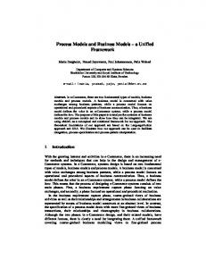
Figure 1 - Alignment of words in the multi-precision computation
X.2.5
ALGORITHM DETAILS AND OPTIMIZATIONS
The presented algorithm is a valid multi-precision version of the full-precision algorithm. The multiplication aibj generates a (k+w)-bit vector. The LS bit of this vector is aligned with cj, which means that aibj is shifted j.w bits to the left. Since the
A design framework for scalable and unified multipliers in GF(p) and GF(2m) product has more than w bits, the most-significant k bits are kept in the spill variable. Observe in Figure 1 that the spill must store the values that go across word boundaries (groups of w bits) including the carries from previous additions (carry). The value for the addition carry is computed as:
carry + 3(2 w − 1) + 2( 2 k − 1) ≤ 2 w ⋅ carry + 2 w − 1
carry ≥
2(2 w − 1) + 2(2 k − 1) 2w −1
(11)
which leads to the conclusion that carry has a maximum value of 3, when w is much larger than k, and maximum of 4 when w = k (recall that k ≤ w ). Hence, spill is in the range [0,2(2k-1)+4]. Once the LS k bits of cj are computed, the new value of cj-1 (shifted k bit positions to the right) is generated (Step 6a). Step 6b can be removed if we add one extra zero digit to p and B, and extend the loop in Step 5b by one more iteration. For that, as it was already indicated in the previous section, p and B must be represented using vectors with e+1 words (radix-2w digits). This modification is attractive to reduce the control complexity of hardware operations. As suggested in [16,17], the representation of partial results in Carry-Save (CS) form is beneficial because addition is executed in a fixed time, independent of the precision of the operands. In GF(p) , CS notation is used in all intermediate steps to represent C as two vectors (CC, CS), such that the value C is obtaining adding the two vectors, which means: C = CC + CS . The final result is converted to non-redundant (conventional) representation before it is passes by the final reduction step (Step 7). When operating in GF(2m) the carries are all zeros, since the Φ operator is equivalent to modulo-2 addition of the bit operands. In this case, only the sum vector (CS) contains the result and the carry vector (CC) is zero. The hardware resources used to add the carry vector can be used in the unified architecture to add another bit-vector. This point is made clear later.
X.3. THE ARCHITECTURE The algorithm states that one digit of the multiplier A is scanned in each i-iteration. After the LS word of the intermediate value of C is determined for digit a0 (leastsignificant digit of A), which takes two j-iterations, the computation using a1 can start. In other words, once the inner loop finishes the execution for j=1 in the ith iteration of the outer loop, the (i+1)th iteration of outer loop can immediately start its execution. Therefore, the level of concurrency that can be reached in Montgomery multiplication algorithms (in any field) is very high [16, 17, 8]. The best architecture to reach high throughput consists in several Processing Elements (PEs) in a pipeline organization, each PE computing one i-iteration of the algorithm. In order to enable for a flexible architecture, the number of PEs may be less than the number of digits in A. Each jiteration is computed in one clock cycle. Other researchers already proposed systolic implementations of the Montgomery multiplication algorithm, but these architectures
Alexandre F. Tenca, Erkay Sava and Çetin K. Koç use a huge amount of hardware and do not have the same characteristics of scalability and unification that is part of the proposed architecture. At the beginning of each PE's computation cycle (iteration), the PE receives the LS word of the inputs. Based on these words and the selected field it determines the value q and consequently the multiple of p to be used throughout the computation cycle (steps 3 and 4). Each i-iteration is computed by a PE for e+1 clock cycles. In case the first PE in the pipeline is still working on one iteration when the last PE in the pipeline started to generate its output, the data generated by the last PE are stored in a buffer, waiting for the first PE to finish its job. If there is at least (e + 1) / 2 PEs, the pipeline will be always working and the buffer won't be necessary. In the worst case (i.e. only one PE in the pipeline), an e-word buffer must be used to hold words of the intermediate result (cj). A timing diagram for the multiplication of 7-bit operands is shown in Figure 2 for the word size w=k=1 and 3 PEs. Dots mark the time slots where a PE (stage) is busy. Note that there is a delay of 2 clock cycles between the stage that computes the iteration for ai and the stage for ai+1. At clock cycles 7 and 15, the first PE in the pipeline can not engage in a new computation and thus the data produced by the last PE in the pipeline needs to be stored in a buffer for 3 clock cycles. At clock cycles 10 and 19, the first PE becomes available and computation proceeds. Hence, we need a buffer to hold 6 bits of the partial sum (C) while the first PE is busy.
Figure 2 - An example of pipelined computation for 7-bit operands which illustrates the situation of data buffering and w=1, radix-2 design
Every time data pass through the pipeline with s PEs we call it a pipeline cycle. The multiplication requires u / s pipeline cycles. Considering the previous example, 3 pipeline cycles are needed and, as a consequence, the last two pipeline stages perform extra computation. Recall that C = A ⋅ B ⋅ 2 − m (mod p ) is the definition of the Montgomery multiplication where m is the number of bits considered for the modulus and operands. When this extra computation is considered, the hardware is in fact calculating C = A ⋅ B ⋅ 2 − kn (mod p ) where n = u / s s corresponds to the number of PEs that worked on the data during the multiplication, and kn ≥ m . It is always possible to rearrange the Montgomery settings according to this new Montgomery exponent, namely R = 2 kn (or R = x kn in GF(2m) case). The total computation time, T (clock cycles) is given by:
A design framework for scalable and unified multipliers in GF(p) and GF(2m)
2 T=
m s + e −1 ks m (e + 1) + 2(s − 1) ks
if (e + 1) ≤ 2 s
(12) otherwise
where m / ks corresponds to the number of pipeline cycles, s is the number of PEs in the pipeline (pipeline stages), and k = log 2 (r ) (radix-r system). Notice that the first line of the formula gives the execution time in clock cycles when there is sufficient number of PEs while the second line corresponds to the case when the data must be buffered for a while before entering the pipeline again. In [17] it is discussed how the utilization of PEs is affected by different conditions, such as the number of PEs in the pipeline and the operands' size. An example of the pipeline organization with s PEs is shown in Figure 3. The pipeline of several PEs is called a kernel, because it is the main computational part of the whole multiplier. The multiplier digits (ai), provided serially to the PEs, are not used again in later stages and can be discarded. Therefore, a simple shift register would be sufficient to store A. The content of the memory elements that hold p and B cannot be destroyed and for this reason a circular register is used. The queue element (FIFO) to store C has its maximum capacity determined by the number of pipeline stages (s) and the number of words (e) in operand A. An estimate of the maximum required length of the queue is given as:
L=
e + 1 − 2(s − 1) if ((e + 1) > 2s ) otherwise 1
(13)
The proposed organization has some degrees of freedom and the evaluation of the best design configurations can be found in [26]. Since we intend to design a fully scalable architecture and we do not want to have the multiplier registers as a limiting factor in the design, one can extend the capacity of these registers using external memory for the excessive words. In this case the length of the registers no longer depends on the precision or the number of PEs. The LS operand words are brought from memory to the registers first and the remaining words are stored in the memory and transferred to the multiplier when needed. However, when the memory transfer rate is not sufficient, the pipeline must be stalled while the data is loaded. This condition would not be ideal but it would still be better than forbidding a particular computation based on a limited capacity of registers in the system. The task of loading the long-precision registers must be handled by another part of the system that interfaces with the user or host system, and is beyond the scope of this work. The modular reduction of the result (Step 7) must also be done by another module [21]. As mentioned before, the reduction step can be avoided when the range for input operands is relaxed [27, 28].
Alexandre F. Tenca, Erkay Sava and Çetin K. Koç
Figure 3 - Pipeline organization with s PEs
X.3.1
PROCESSING ELEMENT
The block diagram of a processing element (PE) for the general unified multiplier architecture is shown in Figure 4. The blocks represent the major arithmetic functions performed by a PE. For simplicity, Figure 4 shows the data buses' widths for nonredundant numbers. Redundant number representation implies more bits per bus. Gray boxes represent registers.
Figure 4 - Processing element
The Digit Multiplier DM1 generates the multiples a i ⋅ b j required in the algorithm steps 3 and 5c. The Φ operation is implemented by two layers of multi-precision
A design framework for scalable and unified multipliers in GF(p) and GF(2m) dual-field adders. The main structure of the multi-precision dual-field adder (MPDFA) is shown in Figure 5. It makes use of a basic component called dual-field adder and registers to propagate information from one word operation to another. A carry-ripple adder design is shown in the multi-precision dual-field adder for simplicity. Other types of adder may be used. The design shown in Section 4 uses a Carry-Save adder structure. The Dual-field adder performs bit-wise addition with or without carry, depending on the field. A dual-field full-adder component (3-2 adder) was presented in [8] in a radix-2 version of the unified multiplier. We propose another design alternative in Section 4.2.
Figure 5 - Multi-Precision non-redundant Dual-Field Adder
Digit multiplier DM2 generates the multiples q ⋅ p j (Step 5c), based on the value q generated by f block (Step 4). Steps 6a and 6b of the hardware algorithm are implemented by proper wiring and registers, as shown at the bottom of Figure 4. Function f is used only at the beginning of the PEs computation, and it lies in the critical path of this design. A retiming strategy [21] may be used to reduce the impact of f in the design, as shown in Figure 6. For simplicity, the bus widths are not shown. In this case, a few LS bits of the LS operand words coming to the PE are required in order to obtain enough information to feed function f. The other bits are computed in a second sub-stage. The MP adders A and B work on words of incoming operands in different algorithm steps. While MP adder A is computing the LS bits of word i+1, MP adder B is computing the most-significant bits of word i. Therefore, carry bits are passed between them to perform the multi-precision addition, as shown in the figure. More details about this operation are presented in [21]. This approach adds one extra cycle to the overall pipeline structure, but provides a significant reduction in the critical path. Function f may be moved to the second sub-stage, if such modification results in a reduced critical path delay.
Alexandre F. Tenca, Erkay Sava and Çetin K. Koç
Figure 6 - Retimed Processing Element
X.4. EXAMPLE: A RADIX-8 UNIFIED PE DESIGN In this section the general design framework presented in the previous sections are applied in the design of a radix-8 PE (k=3). CS adders are used to obtain fast addition at the PE level. The presentation of this example is instrumental to give the reader a better idea of the several design aspects that must be decided in the process, and some of the possible alternatives to get the best results out of the general case presented up to now.
X.4.1
DIGIT MULTIPLIERS
The input digits ai are in the digit set D = {0, 1, 2, 3, 4, 5, 6, 7}. In GF(p) it is more convenient to obtain the multiples aiB using signed basic multiples of the form 2kB, such that “hard”' products are generated using at most two basic multiples, such as: 7B = 8B - B, 3B = 2B + B = 4B - B and so on. However, negative multiples cannot be used to generate products in GF(2m). In this field, three values (4B, 2B, and B) must be generated and then added to obtain all possible multiples aB, with a ∈ D . Instead of combining the basic multiples at the digit multiplier level and delivering only one bit-vector (as suggested in Section 3) we propose in this design to generate the basic multiples and send them to the following multi-precision adder. This solution is
A design framework for scalable and unified multipliers in GF(p) and GF(2m) more attractive since the multi-precision adders can be optimized for the extra input operands. Therefore, the proposed digit multiplier has 3 outputs: x, y, and z that represent the basic multiples. Another output neg is used to complete the negation of a multiple, when in GF(p). Output z has no meaning when working in GF(p) since multiples of p in this field can be obtained with only two basic multiples (represented by x and y). When working in GF(2m), all the output vectors are needed to transfer the 4x, 2x, and 1x multiples. The digit multiplier transfer then 2 multiples to the adder when in GF(p) and 3 multiplies when in GF(2m). The fact that the value of z depends on the field is considered in the design of the multi-precision adder. The logic functions performed by the digit multiplier are shown in Table 1. The notation B’ indicates bit complementation. It can be designed using a small logic gate network and multiplexers. In the retimed PE organization, these muxes are split into two parts, each part allocated in the first or second sub-stages. The control signals for the muxes are passed from one sub-stage to another, after one clock cycle delay. Also note that the digit multiplier must work on words of B. The same digit multiplier is used to generate multiples of p.
ai 000 001 010 011 100 101 110 111
X 0 0 0 4B 4B 4B 4B 8B
GF(p) Y z 0 0 B 0 2B 0 B’ 1 0 0 B 0 2B 0 B’ 1
neg 0 0 0 1 0 0 0 1
x 0 0 0 0 4B 4B 4B 4B
GF(2m) y z 0 0 0 B 2B 0 2B B 0 0 0 B 2B 0 2B B
neg 0 0 0 0 0 0 0 0
Table 1 - Function table for digit multiplication
X.4.2
4-INPUT DUAL-FIELD ADDERS
Considering the redundant representation of C (two bit-vectors in GF(p) and one bit-vector in GF(2m)), and the multiples aiB and qM (three bit-vectors in GF(2m) and 2 bit-vectors in GF(p)), 4-input multi-precision adders must be used. They can be designed using the dual-field adder proposed in [8], however, a better design can be obtained when considering all 4 inputs together. The design of the 4-input Dual-Field Adder is shown in Figure 7. It is similar to a 4-to-2 adder with the introduction of the field information. In the radix-2 design [8], only one out of two XOR gates in the critical path performs a valid operation in GF(2m), however, in radix 8, two out of three XOR gates perform a valid operation in this field. This observation indicates that the radix-8 design has a better resource utilization than the unified radix-2 design.
Alexandre F. Tenca, Erkay Sava and Çetin K. Koç
Figure 7 - 4-input Dual-Field Adder design
X.4.3
FUNCTION F
Depending on the field, different values of q are required based on the LS bits of c0 and p0 (Step 4). The values for radix 8, based on a non-redundant representation of the LS bits of c0 and p0 is shown in Table 2. Observe that there are several similarities between the two fields that could be used to optimize the design of this table. Only two bits of p0 are enough to index the table since the LS bit is always 1. The 3 LS bits of c0 are applied in non-redundant form.
LS bits LS bits of p0 in GF(p) c0 001 011 101 111 000 0 0 0 0 001 7 5 3 1 010 6 2 6 2 011 5 7 1 3 100 4 4 4 4 101 3 1 7 5 110 2 6 2 6 111 1 3 5 7
LS bits of p0 in GF(2m) 001 011 101 111 0 0 0 0 1 7 5 3 2 6 2 6 3 1 7 5 4 4 4 4 5 3 1 7 6 2 6 2 7 5 3 1
Table 2- Function f - generation of q
X.4.4
COMPLETE DESIGN
A block diagram for the radix-8 PE is shown in Figure 8. It puts together the digit multipliers presented in Section 4.1, the multi-precision adders using 4-input dual-field adders discussed in Section 4.2, and the function f presented in Section 4.3. Muxes are used to select proper inputs for the multi-operand addition, according to the field.
A design framework for scalable and unified multipliers in GF(p) and GF(2m) Using these muxes we reduce the number of inputs in the multi-precision adder to only 4. The use of the muxes is possible because output z of the digit multiplier is zero when in GF(p) and carry bits are zeros in GF(2m).
Figure 8- Radix-8 Processing Element Block Diagram
X.5. EXPERIMENTAL RESULTS AND EVALUATION The radix-8 unified design was described using VHDL and synthesized using Mentor Graphics tools for a 0.5 m AMI CMOS technology (ADK library [29]). The tool incorporates an estimate of wire delays and for this reason, an actual chip implementation may show some small variation on the timing presented in this section. Based on the highly modular design, the critical path of a PE defines the minimal clock period that can be applied to the pipeline. Other components in the design, such as the one responsible for final reduction, may be pipelined to match the PE critical path delay. Table 3 shows the area (in equivalent gates, i.e. 2-input NAND gates) and delay of some PE designs, using different word size (w). Observe that the word size is not affecting the critical path because CS representation of intermediate results was used.
W 8 16 32
Unified Architecture Area (gates) Critical Path (ns) 1138 (14%) 9.84 1993 (12%) 9.84 3646 (11%) 9.84
Only GF(p) [21] Area (gates) Critical Path (ns) 999 8.32 1787 8.32 3280 8.32
Table 3 - Area/time values for PEs synthesized for 0.5 m AMI CMOS technology
Alexandre F. Tenca, Erkay Sava and Çetin K. Koç An important parameter for evaluation consists in comparing a multiplier designed only for GF(p) with the unified multiplier. The design proposed in [21] uses radix 8 and works in GF(p) only. The unified design was synthesized for the same technology, using the same tools. The synthesis results are also shown in Table 3. The Table shows that the increase in area from an architecture designed only for GF(p) to the unified architecture is only 11% to 14%. The delay in the critical path increased by 18%, with a consequent reduction of 15% in maximum clock frequency at which the system can operate. It was expected to find that the unified architecture would be slower and more area consuming then the non-unified one, and the results obtained from this analysis show that it is not a big price to be paid for all the extra functionality provided by the unified architecture. Several kernel configurations may be obtained using different number of PEs or varying the word size used by the PE. The total area of the kernel is linearly dependent on the number of PEs. The total number of cycles to perform a modular multiplication on n-bit operands will depend on the kernel configuration. Table 4 shows the number of clock cycles to perform the operation for some typical n values and some chosen kernel configurations (with approximately 30,000 gates). Observe that the hardware is capable of executing in 0.8 to 1.8 clock cycles/bit. A reconfigurable architecture shown in [30] works at a speed of 1 clock cycle/bit. It is important to say that the design in [30] has extended functionality (performs more than just multiplication) and it has an estimated area (our estimate) for the data path (excluding registers and I/O interface) of roughly 440,000 devices (110,000 gates). This reconfigurable processor executes operations in GF(2m) at the same speed as the operations in GF(p), the same way it is done in the proposed architecture. Multiplication in GF(2m) is done using conventional methods (not Montgomery multiplication).
n 128 256 512 1024
Kernel configurations (w,s) (8,25) (16,15) (32,8) (64,4) 116 98 100 90 232 196 184 180 510 436 410 436 1868 1546 1476 1554
Table 4 - Clock cycles to perform modular multiplication in GF(p) or GF(2m) (radix 8)
A comparison of the speed of a radix-2 unified design with a microprocessor-based implementation of MM in GF(p) was presented in [8] and demonstrates that a radix-2 design can be almost 10 times faster than an ARM microprocessor at 80MHz when performing multiplication. The proposed radix-8 design could be therefore almost 30 times faster when working at the same frequency. Notice that the proposed design can work at much higher clock frequency. Since the multiplier design for GF(p) is the most complex one, it establishes the lower bound on the unified architecture complexity. It is clear that the unified design will yield less performance than other specific hardware designs proposed for GF(2m) multiplication only.
A design framework for scalable and unified multipliers in GF(p) and GF(2m) The choice of the radix impacts the design complexity and it is not the goal of this work to investigate the effect of different radices in the system performance. The radix8 example was taken to allow a better presentation of the concepts. A fair comparison between the radix-2 unified architecture in [8] and this radix-8 architecture would require re-synthesizing the radix-2 design. Nevertheless, it was shown in [21] that the radix-8 design for GF(p) has a better area/time factor than the radix-2 design for the same scalable architecture. Another question is related to the kernel configuration that provides the best area/time relation. This problem has been investigated in [26]. The best configuration depends on the operand precision for which the multiplier is used the most. For example, if the multiplier is optimized for 1024-bit numbers, and a maximum area of 30,000 gates, the configuration that provides the best result is p=8 and w=32 (14.5 sec). For 256 bits, the configuration should be p=2 and w=128 (1.7 sec). Both cases obtained trying to get the best time from the architecture using the given area. Recall that even though we optimize the configuration for a given precision, other values of precision are still possible. In general, optimizing the design for the largest precision is the best choice. For example: the configuration p=8 and w=32 performs multiplication on 256-bit operands in 1.8 secs, just slightly slower than the best configuration of p=2 and w=128.
X.6. SUMMARY This chapter presented a design framework to obtain scalable and unified modular multipliers based on Montgomery multiplication algorithm. These multipliers are able to work in both GF(p) and GF(2m) . The advantage of this approach resides on the flexibility of the proposed solution. The resulting designs allow the use of any modulus value or any irreducible polynomial. This feature is important for cryptosystems using ECC and RSA that require added security. The design is highly scalable allowing the designer to create a system that fits a particular area and extract a good level of performance from the available silicon. Any precision of the operands is allowed, up to a maximum system memory capacity. The kernel itself is designed to handle an unlimited precision of the operands. Our experiments show that the speed of our design example using radix-8 digits is very good with significantly less area than other approaches, and still offering a lot of flexibility. Previous work on a radix-2 architecture shows that the unified design is able to run almost 10 times faster than an optimized code on an ARM microprocessor. The generalization of unified architectures for any radix, as proposed in this text, opens the door to the investigation of the impact of other radices in the system performance, and the exploration of several alternatives for the implementation of system components, such as adders and digit multipliers.
References: [1] J.-J. Quisquater and C. Couvreur, “Fast decipherment algorithm for RSA public-key cryptosystem,” IEE Electronics Letters, vol. 18, no. 21, October 1982, pp. 905-907.
Alexandre F. Tenca, Erkay Sava and Çetin K. Koç [2] W. Diffie and M. E. Hellman, “New directions in cryptography,” IEEE Transactions on Information Theory, vol. 22, November 1976, pp. 644-654. [3] National Institute for Standards and Technology, “Digital signature standard (DSS),” Federal Register, August 1991. [4] N. Koblitz, “Elliptic curve cryptosystems,” Mathematics of Computation, vol. 48, no. 177, January 1987, pp. 203-209. [5] A. J. Menezes, Elliptic Curve Public Key Cryptosystems, Kluwer Academic Publishers, Boston, MA, 1993. [6] P. L. Montgomery, “Modular multiplication without trial division,” Mathematics of Computation, vol. 44, no. 170, April 1985, pp. 519-521. [7] Ç. K. Koç and T. Acar, “Montgomery multiplication in GF(2k),” Designs, Codes and Cryptography, vol. 14, no. 1, April 1998, pp. 57-69. [8] E. Sava , A. F. Tenca, and Ç. K. Koç, “A scalable and unified multiplier architecture for finite fields GF(p) and GF(2m),” Lecture Notes in Computer Science Cryptographic Hardware and Embedded System - CHES' 2000, Ç. K. Koç and Christof Paar, Eds. 2000, vol. 1965, pp. 277-292, Springer, Berlin, Germany. [9] H. Orup, “Simplifying quotient determination in high-radix modular multiplication,” 12th Symposium on Computer Arithmetic, Knowles S and W. H. McAllister (Eds.), Bath, England, July 1995, pp. 193-199, IEEE Computer Society Press. [10] Ç. K. Koç, T. Acar, and B. S. Kaliski, “Analyzing and comparing Montgomery multiplication algorithms,” IEEE Micro, vol. 16, no. 3, June 1996, pp. 26-33. [11] A. Bernal and A. Guyot, “Design of a modular multiplier based on Montgomery's algorithm,” 13th Conference on Design of Circuits and Integrated Systems, Madrid, Spain, November 17-20 1998, pp. 680-685. [12] S. E. Eldridge and C. D. Walter, “Hardware implementation of Montgomery's modular multiplication algorithm,” IEEE Transactions on Computers, vol. 42, no. 6, June 1993, pp. 693-699. [13] P. Kornerup, “High-radix modular multiplication for cryptosystems,” 11th Symposium on Computer Arithmetic, E. Swartzlander, Jr., M. J. Irwin, and G. Jullien (Eds.), Windsor, Ontario, June 29 - July 2 1993, pp. 277-283, IEEE Computer Society Press. [14] A. Royo, J. Moran, and J. C. Lopez, “Design and implementation of a coprocessor for cryptographic applications,” European Design and Test Conference, Paris, France, March 17-20 1997, pp. 213-217. [15] C. D. Walter, “Space/Time trade-offs for higher radix modular multiplication using repeated addition,” IEEE Transactions on Computers, vol. 46, no. 2, February 1997, pp. 139-141. [16] A. F. Tenca and Ç. K. Koç, “A Scalable Architecture for Modular Multiplication Based on Montgomery's Algorithm,” IEEE Transactions on Computers, vol. 52, no. 9, September 2003, pp. 1215-1221. [17] A. F. Tenca and Ç. K. Koç, “A scalable architecture for Montgomery multiplication,” Lecture Notes in Computer Science, 1999, vol. 1717 Workshop on Cryptographic Hardware and Embedded Systems - CHES' 99, pp. 94-108, Springer, Berlin, Germany. [18] G. B. Agnew, R. C. Mullin, and S. A. Vanstone, “An implementation of elliptic curve cryptosystems over F2155 ,” IEEE Journal on Selected Areas in Communications, vol. 11, no. 5, pp. 804-813, June 1993. [19] D. Naccache and D. M'Raihi, “Cryptographic smart cards,” IEEE Micro, vol. 16, no. 3, June 1996, pp. 14-24. [20] M. Jacobson, A. J. Menezes, and A. Stein, “Solving elliptic curve discrete logarithm problems using Weil descent,” CACR Technical Report CORR2001-31, University of Waterloo, May 2001.
A design framework for scalable and unified multipliers in GF(p) and GF(2m) [21] A. F. Tenca, G. Todorov, and Ç. K. Koç, “High-radix design of a scalable modular multiplier,” Cryptographic Hardware and Embedded Systems - CHES' 2001, Ç. K. Koç, D. Naccache, and C. Paar (Eds.), Paris, France, May 2001, Lecture Notes in Computer Science, No. 2162, pp. 185-201, Springer, Berlin, Germany. [22] H. Wu, “Montgomery multiplier and squarer in GF(2m),” Cryptographic Hardware and Embedded Systems, Ç. K. Koç and C. Paar (Eds.) 1999, Lecture Notes in Computer Science, No. 1965, pp. 264-276, Springer, Berlin, Germany. [23] J.-H. Oh and S.-J. Moon, “Modular multiplication method,” IEEE Proceedings, vol. 145, no. 4, July 1998, pp. 317-318. [24] B. S. Kaliski Jr., “The Montgomery inverse and its applications,” IEEE Transactions on Computers, vol. 44, no. 8, August 1995, pp. 1064-1065. [25] E. Sava and Ç. K. Koç, “The Montgomery inversion - revisited,” IEEE Transactions on Computers, vol. 49, no. 7, July 2000, pp. 763-766. [26] B. Kurniawan, “ASIC design and implementation of a parallel exponentiation algorithm using optimized scalable Montgomery multipliers,” M.S. thesis, Oregon State University, Corvallis, Oregon, USA, 2002. [27] G. Hachez and J.-J. Quisquater, “Montgomery exponentiation with no final subtractions: improved results,” Lecture Notes in Computer Science - Cryptographic Hardware and Embedded System - CHES' 2000, Ç. K. Koç and C. Paar (Eds.), 2000, vol. 1965, pp. 293-301, Springer, Berlin, Germany. [28] C. D. Walter, “Montgomery exponentiation needs no final subtractions,” IEE Electronics Letters, vol. 35, no. 21, October 1999, pp. 1831-1832. [29] ASIC Design Kit. Mentor Graphics Co., “ADK documentation,” obtained from http://www.mentor.com/partners/hep/AsicDesignKit/ASICindex.html. [30] J. Goodman and A. P. Chandrakasan, “An energy-efficient reconfigurable public-key cryptography processor,” IEEE Journal of Solid-State Circuits, vol. 36, no. 11, 2001, pp. 1808-1820.