Currently, they fall into two categories: firstly, algorithms based on methods from computer graphics which use e.g. mesh parametrizations, evolving surfaces or ...
A FRAMEWORK FOR SCENE-FLOW DRIVEN CREATION OF TIME-CONSISTENT DYNAMIC 3D OBJECTS USING MESH PARAMETRIZATIONS Patrick Klie
Eugen Okon
Nikolˇce Stefanoski
J¨orn Ostermann
Leibniz Universit¨at Hannover Institut f¨ur Informationsverarbeitung Appelstr. 9A, 30167 Hannover, Germany Email: {klie|okon|stefanos}@tnt.uni-hannover.de ABSTRACT
2. RELATED WORK
In this paper we propose a novel method to create dynamic mesh sequences with fixed connectivity from multiple camera video streams. Fixed connectivity is useful for dynamic mesh coding as mesh connectivity has to be transmitted only once and not frame-wise. The proposed method runs automatically. It deploys mesh parametrizations and voronoi diagrams from the computer graphics realm as well as 2D optical and 3D scene flow from computer vision. Assuming a given dynamic mesh sequence not necessarily having constant connectivity, motion estimation is performed by applying a 3D motion field to a static reconstruction in one frame. Afterwards, mesh connectivity is transferred patch-wise from one frame to the next one using remeshing techniques. The entire method is independent of static mesh resolution, hence supplying a basis for dynamic mesh coding and simplification.
Some methods exist to create fixed connectivity or at least animated meshes. Currently, they fall into two categories: firstly, algorithms based on methods from computer graphics which use e.g. mesh parametrizations, evolving surfaces or geodesic distance conservation. Secondly, there are methods from the computer vision realm which perform some kind of a 3D motion estimation and tracking applying this motion information to the underlying geometric data. In our approach we try to combine advantages from both realms. Bronstein et al. [1] create intrinsic correspondences between animated 3D faces as the minimum-distortion mapping. They use generalized ”Multidimensional scaling” for this goal. In [2], Adela C. Gonz´alez generally describes means to obtain constant connectivity mainly based on Deformable Objects, the deformation itself is driven by physics describing the instantaneous potential energy of the body elastic deformation. Anuar and Guskov propagate a single mesh template through time fitting it to the input surface data using signed distance transforms, Bayesian motion estimation and vector fields [3]. In [4], Summer and Popovic describe how to transfer the deformation exhibited by a source triangle mesh onto a different target triangle mesh. The meshes do not have to share the same connectivity. Correspondence has to be set by the user interactively on a small set of vertex markers. The deformation is done by solving an optimization problem to consistently apply the transformations to the target shape.
Index Terms— 3d motion analysis and tracking, surface modeling for 3-D scenes, multi-view image and 3D data processing, 3D mesh representation, 3D motion animation
1. INTRODUCTION Coding realm is emanating from image, audio and video coding to coding of 3D objects. While compression of static 3D objects has been studied thoroughly in the past, coding of dynamic 3D objects is currently emerging and of increasing interest in the context of 3DTV, medical visualization, tele-conferencing, free viewpoint video, and view synthesis. One of the crucial point in coding of dynamic 3D objects is the so called time consistency, i.e. representing a dynamic 3D object as a series of static 3D meshes with non-changing connectivity, while vertex locations
3. ALGORITHM OVERVIEW The partial steps of the algorithm are described in this section. Mainly, the calculations are made on two static reconstructions at time steps n, n + 1.
F p11 , . . . , p1V , . . . , pf1 , . . . , pfV , . . . , pF 1 , . . . , pV ,
(F : number of frames, V : number of vertices) change their location in time. Most of the static reconstruction methods create a mesh with a specific connectivity so there is no straight-forward transition from static to dynamic reconstruction concerning the conservation of connectivity. The question arises how to obtain this time consistency. This work is supported by the EC within FP6 under Grant 511568 with the acronym 3DTV.
3.1. Static Mesh Reconstruction The static reconstructions are obtained via classical silhouette intersections. We do not use any voxel based methods to avoid quantization inaccuracy but rather perform boolean operations directly on the silhouette cones (see figure 1 (a)) similar to the method proposed in [5]. The results are only very coarse representations of the object (figure 1 (b)), so we apply dense depth maps from every camera view to carve out concavities and enhance mesh accuracy (figure 1 (c)). We currently use the synthetic multi-view data set known as the ”kung fu girl” supplied by the Max Planck Institute in Saarbr¨ucken.
(a) Silhouette cones
(a) Found good features to track
(b) Voxel-free silhouette intersection
(b) Tracked features
(c) Refined mesh
Fig. 1. Static reconstructions (c) 3D scene flow In the near future we will use real world data obtained by our multi camera studio described in [6].
Fig. 2. From optical flow to scene flow
3.2. 3D motion estimation According to Vedula et al. [7, 8], threedimensional scene flow can be calculated from multiple optical flows. They describe three major scenarios where 3D scene flow can be calculated: • Complete knowledge of the scene structure and rate of change of depth maps • Stereo or multi-view correspondences • No knowledge of the scene structure at all Fortunately, the first scenario takes place in our case as we have the static reconstructions for every time step, and the depth maps can be obtained by multi-view stereo. Scene flow calculation dx for this case is mainly based on opdt i tical flow du , differential change between surface points and 2D dt ∂x points in the camera target expressed as an inverse Jacobian ∂u , i ˛ ∂x ˛ and temporal derivative of the surface depth map ∂t u : i
˛ dx ∂x dui ∂x ˛˛ = + dt ∂ui dt ∂t ˛ui The 2D flow vectors are calculated on good features to track [9], and therefore yield a non-dense motion field compared to image and mesh resolution. Some of the features are lost, but most of them are tracked and can be used as optical flow vectors (see figure 2). The inverse Jacobian could be estimated by using the surface gradient ∇f and a set of 6 linear equations described in [7, 8], but we project the ”flowed” points onto the surface using ray-surface intersections instead (figure 2 (c)). We prolong or shorten the flow vectors to get intersections with the two static reconstructions. The intersection points define ”anchor points” where a local 1-to-3 split is performed (see figure 3). These additional vertices are removed afterwards as they do not belong to the original mesh connectivity.
Fig. 3. Local subdivision at anchor point positions
The problem arises that the anchor points define a very sparse subset of the set of the vertices and hence, we do not have any motion information for a large number of vertices. The proposed solution to this is to use the motion vectors for an entire neighborhood around these anchor points. 3.3. Mesh segmentation After having calculated 3D scene flow vectors, we perform mesh segmentations to get what we call ”similarity registration”. The anchor points in both time steps define seed points on both meshes we use to calculate discretized voronoi diagrams on (compare [10]). If we assume that the surface deformation is completely isometric then isometry is inherited to the corresponding surface patches. If isometry is violated locally or globally in a physically plausible sense, the surface patches still remain in a valid relation to each other due to the voronoi property. Regions of isometry violation without any motion information are canditates for high tangential drift, while anchor point correspondence together with the voronoi property provides a clue to recognize geodesic distance change in a sub-sampled fashion.
As the seeds are defined on vertices rather than on triangles, region growing is done via adding derived neighbourhoods (figure 4, dashed lines) for the vertices described in [11] yielding patch boundaries along sub-vertex positions (see figure 4).
(a) Corresponding surface patches in time step 13 and 14
(b) Parametrization of corresponding surface patches Fig. 4. Derived neighborhoods of vertices The algorithm stops if the entire meshes are covered with voronoi tiles. In order to get real triangulations for every surface patch, the border regions of the patches are locally subdivided, and the additionally created vertices, edges and faces are marked for later removal as they do not belong to the original mesh connectivity either. The result of this partial step is patch correspondence in the sense that each pair of patches has one inherent 3D motion vector. 3.4. Mesh Parametrization and Remeshing The resulting patches are then parameterized separately onto convex forms An , An+1 , e.g. rectangles or circles (see figure 5 (b)). A following remeshing from An to An+1 result in a patch-wise transfer of the connectivity from time step n to time step n + 1 (see figure 5 (c)). The connectivity is taken from the first surface patch, while the geometry information comes from the second one. The remeshing is done by simple barycentric interpolation relative to the 1-ring of vertices. We use standard parametrization methods developed by Floater [12]. As every vertex of the mesh in time step n gets a new position in time step n + 1, the result is a dense 3D motion vector field giving us motion information on every vertex of the mesh (first three pictures of figure 6). 3.5. Filtering of Motion Trajectories If motion field vectors for every time step are concatenated one after another through time, we get motion trajectories for every vertex of the mesh. These trajectories tend to be very noisy, so we apply low pass filters to the trajectories in a post processing step to obtain smooth transitions. 4. RESULTS In figure 5 (a) a surface patch with 76 triangles from time step 13 in the area of the hand is depicted exemplarily. Figure 5 (a) also shows the corresponding surface patch in time step 14 with 27 triangles. The parametrizations and the remeshing can be seen in 5 (b), (c). Figure 6 depicts a flowed surface patch together with the dense motion information. The target mesh is drawn in wireframe mode for better clarity.
(c) Remeshed surface patch Fig. 5. Parametrization and Remeshing of Surface Patches
5. CONCLUSIONS We present a novel method to create mesh sequences with constant connectivity using a combination of well-known techniques from both computer graphics and computer vision. As a side effect, we get a threedimensional non-rigid motion estimation which can be used for other purposes such as 3D motion compensation. The main assumption is that object surface is constrained to isometry during movements. If isometry is violated, the method still works but produces mesh distortions making many texture coordinate recalculations necessary in case of texturing the 3D object. The method still does not guarantee total tangential drift control. Also, it heavily depends on the number and the quality of the 2D optical flow vectors and the dense depth maps. If optical flow lacks due to motion blur, the entire algorithm fails. The practical consequence of this is to find the optimum between studio light, aperture of the camera lenses and shutter time. The algorithm to calculate 3D scene flow depends on the surfaces being Lambertian reflectors, so the light should not be too shiny. Shutter time has to be short enough to avoid motion blur but also long enough not to darken everything. We currently use maximal aperture size of 1.4 to make short shutter times possible but restricting action range of movements to a very narrow depth of focus. We try to come up with this by using diffuse studio lights and a treadmill in the middle of the multi camera studio to simulate movements without getting out of focus.
[3] Nizam Anuar and Igor Guskov, “Extracting animated meshes with adaptive motion estimation.,” in VMV, 2004, pp. 63–71. [4] Robert W. Sumner and Jovan Popovi´c, “Deformation transfer for triangle meshes,” ACM Trans. Graph., vol. 23, no. 3, pp. 399–405, 2004. [5] Wojciech Matusik, Chris Buehler, and Leonard McMillan, “Polyhedral visual hulls for Real-Time rendering,” in 12th Eurographics Workshop on Rendering Techniques, 2001, pp. 115–126. [6] Patrick Klie, Torsten B¨uschenfeld, and J¨orn Ostermann, “Vipid - virtual 3d person models for intuitive dialog systems,” in IEEE Workshop on Content Generation and Coding for 3Dtelevision, jun 2006, vol. 1. [7] Sundar Vedula, Simon Baker, Peter Rander, Robert Collins, and Takeo Kanade, “Three-dimensional scene flow,” IEEE Transactions on Pattern Analysis and Machine Intelligence, vol. 27, no. 3, pp. 475 – 480, March 2005. [8] Sundar Vedula, Simon Baker, Peter Rander, Robert Collins, and Takeo Kanade, “Three-dimensional scene flow,” in ICCV (2), 1999, pp. 722–729. [9] Jianbo Shi and Carlo Tomasi, “Good features to track,” in 1994 IEEE Conference on Computer Vision and Pattern Recognition (CVPR’94), 1994, pp. 593 – 600. (a) ”Flowed” surface patch Fig. 6. Dense non-rigid 3D motion vector field
6. OUTLOOK AND FUTURE WORK The tangential drift control is one of the upcoming problems to be addressed. This is important for several reasons. For instance, fewer texture coordinate recalculations are necessary. Also, motion analysis based on 3D scene flow regarded as a vector field, is more robust when tangential drift is eliminated. There are situations where constant connectivity cannot be uphold or isn’t even desired, e.g. in cases of self collision. Transferring the entire mesh connectivity would be very costful. Therefore we will define a set of streamable operations to come up with local topological and connectivity changes. 7. ACKNOWLEDGEMENT The authors would like to thank the EC IST 6th Framework 3DTV NoE for partially funding this work. Additional thanks go to the GrOVis group of the Max Planck Institute in Saarbr¨ucken for their synthetic multi view data set ”Kung-Fu Girl”. 8. REFERENCES [1] M. M. Bronstein, A. M. Bronstein, and R. Kimmel, “Face2face: an isometric model for facial animation,” in Proc. Conf. on Articulated Motion and Deformable Objects (AMDO), 2006, pp. 38–47. [2] Adela C. Gonz´alez, JCS&T, 2002.
“Generation of flexible 3D objects,”
[10] Matthias Eck, Tony DeRose, Tom Duchamp, Hugues Hoppe, Michael Lounsbery, and Werner Stuetzle, “Multiresolution analysis of arbitrary meshes,” Computer Graphics, vol. 29, no. Annual Conference Series, pp. 173–182, 1995. [11] A. KLEIN, A. CERTAIN, T. DEROSE, T. DUCHAMP, and W. STUETZLE, “Vertex-based delaunay triangulation of meshes of arbitrary topological type,” 1997. [12] Michael S. Floater, “Parametrization and smooth approximation of surface triangulations,” Computer Aided Geometric Design, vol. 14, no. 4, pp. 231–250, 1997.