ery peer p will maintain a pointer to the successor of its identifier p plus one, i.e.. succP (pâ1). Similarly, each ...... mic lookup length becomes trivial. Also, the ...
A Framework for Structured Peer-to-Peer Overlay Networks ? Luc Onana Alima1,2 , Ali Ghodsi1,2 , and Seif Haridi1,2 1 2
IMIT-Royal Institute of Technology (KTH) Swedish Institute of Computer Science (SICS) {onana,ali,seif}@sics.se SICS Technical Report T2004:09 ISSN 1100-3154 ISRN:SICS-T–2004/09-SE
Abstract Structured peer-to-peer overlay networks have recently emerged as good candidate infrastructure for building novel large-scale and robust Internet applications in which participating peers share computing resources as equals. In the past three year, various structured peer-to-peer overlay networks have been proposed, and probably more are to come. We present a framework for understanding, analyzing and designing structured peer-to-peer overlay networks. The main objective of the paper is to provide practical guidelines for the design of structured overlay networks by identifying a fundamental element in the construction of overlay networks: the embedding of k−ary trees. Then, a number of effective techniques for maintaining these overlay networks are discussed. The proposed framework has been effective in the development of the DKS system, whose preliminary design appears in [2].
1. Introduction The exponential growth of the Internet has made it possible to connect billions of machines scattered around the globe and to share computing resources such as processing power, storage and content. In order to effectively exploit these resources, the trend is to use the Internet as it was originally intended. That is, a symmetric network through which machines share resources as equals. With this in mind, a number of novel distributed systems/applications characterized by large-scale and high-dynamism of their operating environment are being built. In these distributed systems, participating peers directly share resources as equals in a peer-to-peer fashion [7, 5, 17]. We name them, peer-to-peer (P2P) systems. The high dynamism in P2P systems is due to two reasons mainly. First, there is the need for freedom, peers should be able to join or leave the system at any time. Second, peers or the underlying communication network, which is typically the ?
This work was funded by the European project IST-2001-32234, PEPITO, the European project EVERGROW IST-2004-001935, the Vinnova projects PPC and GES3 in Sweden.
Internet, can fail at any time. To cope with this dynamism, these systems should be stabilizing, that is, despite the high-dynamism, the system should converge to legitimate configurations, without external intervention. Peer-to-peer systems are attractive in at least two respects. First, from the user standpoint, peer-to-peer computing has a huge potential, as it reduces the need for expensive back-end servers, typically used to perform complex tasks. Moreover, the administrative costs are significantly reduced, as peer-to-peer systems are in general built on autonomous systems, without a centralized administration. Second, from the scientific perspective, peer-to-peer systems are large-scale distributed systems that involve challenging issues such as fault-tolerance, scalability and security. The current trend in building P2P systems, consists in providing an applicationindependent overlay network as a substrate on top of which novel large-scale applications can be constructed. An overlay network is a logical network on top of one or more networks. A well-known example of such networks is the Internet. The main purpose of an overlay network is to provide effective means by which a huge amount of computing resources are linked together and accessed. And, as can be seen nowadays, various high-level distributed services can be built on top of an overlay network [6, 3, 13]. The performance of these high-level distributed services strongly depends on the properties of the underlying overlay network. Two main design approaches can be identified for building overlay networks. On the one hand, there are un-structured overlay networks [14, 11], in which peers are extremely autonomous. That is, a peer joins the overlay network by connecting itself to any other existing peers. We say that un-structured overlay networks are built in an un-controlled fashion. Unstructured overlay networks have the advantage of providing flexibility when it comes to finding resources within the system. For instance, arbitrary queries can be handled easily. However, they provide restricted guarantees, because even if a data item were inserted into the system, there is no guarantee that it will be located when needed. Furthermore, these overlay networks tend to be inefficient, as they mainly use flooding for search. On the other hand, there are structured overlay networks [26, 23, 24, 2, 1, 19], where a peer joins the overlay network by connecting itself to some other well-defined peers, based on its logical identifier. We say that structured overlay networks are built in a controlled manner. These overlay networks provide high guarantees but have a limited query language. For example, complex queries are not supported in a “natural” way. In this paper, our focus is on structured overlay networks [25, 2, 24]. Hence, we will use the term overlay network to mean structured overlay network. The core service that these overlay networks provide is a location-independent virtual identifier basedrouting3 . That is, given a message along with a virtual identifier vid, the overlay network routes the message to the ultimate destination dest(vid), which is related to vid in a well-defined manner. We discuss the relation between vid and dest(vid) in Section 2.3. On top of the core service mentioned above, a number of high-level services such as Distributed Hash Table (DHT), location-independent one-to-one communication (point-to-point), one-to-many communication such as broadcast [13, 10] and multicast [4], object replication and caching under various consistency models can be built. 3
In [8], the term key-based routing is used in place of virtual identifier based routing.
2
1.1. Motivations Since the introduction of structured overlay networks, various such systems have been proposed. A partial list includes [26, 23, 24, 2, 1, 19, 16, 18, 21], and new such systems are probably to come. Unfortunately, existing structured overlay networks are presented in a fragmented way. As a consequence of this, understanding any new such systems requires significant efforts. Furthermore, the analysis of, as well as the comparison between, overlay networks becomes difficult. And, in many cases, designing novel structured overlay networks amounts to re-inventing. A careful analysis of most of the existing structured overlay networks reveals at least the following common characteristics: (i) Logarithmic diameter. All existing structured overlay network designs we know of strive to achieve (very) large networks with logarithmic diameter while maintaining, at each peer, a compact routing table. Typically, the routing table at each peer is either of logarithmic or constant size. How the logarithmic diameter is ensured varies (apparently) from one system to another. Hence, to analyze the performance (in terms of overlay hops) of any new system, significant efforts has to be re-invested. Therefore, there is a need to identify any unifying fundamental concept behind the achievement of logarithmic degree. (ii) Convergence/Stabilization To cope with the high dynamism, structured overlay networks are designed to be convergent (or stabilizing). That is, if ever the dynamism were ceased, the overlay network should self-configures to reach and remain in legitimate configurations. And, even if the dynamism were not stopped, the network should still route messages with acceptable performance. To achieve this convergence or stabilization property, practical maintenance techniques are needed.
1.2. Contributions The motivations presented above point out two important aspects in which we contribute. We propose a small set of practical design principles for understanding, analyzing, building and maintaining structured overlay networks. The contributions of this paper is the embedding of k-ary trees4 . To simplify the understanding of the logarithmic diameter, we propose the embedding of k-ary trees as the fundamental concept. Briefly and intuitively, the idea is to let each peer be the root of directed acyclic graph that spans the whole system. We conjecture that any structured overlay network that ensures logarithmic diameter under normal system operation (in a deterministic fashion), is such that each peer is the root of an embedded k-ary tree along which a form of interval/compact routing [27] is exploited. In addition to the embedding of k−ary trees, we elaborate on the following techniques introduced in [2],[12]: 4
In this paper, we abuse the terminology. We often use the term tree where the term rooted DAG (Directed Acyclic Graph) should be used.
3
(ii) Local atomic operation: To reduce disturbances when peers join and leave the system, we propose that the join as well as the leave operation be managed by restricted atomic operation that involve only a small part of the overlay network. (iii) Correction-on-use: The use of local atomic operation does not guarantee that the system will “immediately” be in legitimate configurations whenever peers join or leave the system. Anyway, this cannot be achieved in an asynchronous distributed system. So, because of joins, leaves and failures, routing table at peers become inaccurate. We propose the correction-on-use technique as the basic technique for maintaining structured overlay networks. With this technique, unnecessary bandwidth consumption is avoided. And, for the system to perform optimally even under perturbation, the injected traffic should be high enough. (iv) Correction-on-change: With correction-on-change, whenever a change occurs in the system, all the peers that need to be updated are notified. The main challenge is to find, efficiently, those peers that need to be updated. Moreover, the notification should be performed in an efficient way. We provide effective mechanisms both for identification of the peers that need to be updated and for the notification.
1.3. Road-map The rest of this paper is organized as follows. Section 2 summarizes the steps to be considered when designing structured overlay networks. In Section 3, we present the principle for embedding k−ary trees in a virtual identifier space. The embedding of k−ary trees relies on the division of the virtual space that be either relative or fixed. Section 4 presents the relative division of the space. In section 5 we present the fixed division of the space. Section 6 is devoted to the principle of local atomic operation, for joins and leaves of peers. In Section 7, we present different techniques for maintaining structured overlay networks. Section 8 concludes the paper and points out some ongoing and future work.
2. Steps in Designing Structured Overlay Networks The steps in designing structured overlay networks are summarized in Figure 1. An analysis of most of the existing structured overlay networks show that there are a number of key design decisions that are to be considered, when building a structured overlay network. We elaborate on these steps in this section.
2.1. Decide an Identifier Space Perhaps the first design decision to be made when designing a structured overlay network is to decide on what will be the the virtual identifier space. Throughout this document, we will use I to denote the identifier space. The choice of the virtual identifier space is motivated by several reasons. 1. Addressing: the identifier space plays the role of an address space, used for identifying resources to be interconnected by the overlay network. Each computing 4
Fig. 1. a) Use F2 to map items onto the identifier space. Use F1 to map peers to the identifier space. Decide an assignment of items to peers. Use an embedding of k−ary tree to interconnect the peers.
resource participating in a structured overlay network receives a virtual identifier taken from the virtual identifier space, I. 2. Scalability. To provide access to very large sets of resources the identifier space is chosen to be a very large virtual space. This is simply an application of the well-known principle of indirection for achieving (numerical [22]) scalability, as was done for the Internet. Typically, the size |I| = N is in O(k d ), for k ≥ 2, and some large positive integer d. Hence for a fixed k, the size of the virtual space grows exponentially with base k. 3. Location-Independent Communication. Another important aspect of the virtual identifier space is that it allows peers present in the system to communicate in a point-to-point or one-to-many manner irrespective of their actual location. Thereby allowing for pure mobility. The identifier space is assumed to have some “distance”, denoted ∆ in this paper. Formally, ∆ is a function of type ∆ : I × I → R, where R denotes the set of real numbers. It is required that ∆ satisfies at least the following three properties (D1 ) : (∀x, y : x, y ∈ I : ∆(x, y) ≥ 0). (D2 ) : (∀x : x ∈ I : ∆(x, x) = 0). (D3 ) : (∀x, y : x, y ∈ I : ∆(x, y) = 0 ⇒ x = y). and if possible, ∆ can also satisfy the following two properties: (D4 ) : (∀x, y : x, y ∈ I : ∆(x, y) = ∆(y, x)). (D5 ) : (∀x, y, z : x, y, z ∈ I : ∆(x, z) ≤ ∆(x, y) + ∆(y, z)). In case ∆ satisfies all the above five properties, we have that (I, ∆) is a metric space. However, in general this is not the case. In this paper, we shall say that (I, ∆) is 5
a “pseudo-metric” space to mean that properties (D1 ), (D2 ), (D3 ) are satisfied and possibly (D4 ) and (D5 ). The closeness metric, ∆, defined on the identifier space serves two purposes: – clustering of resources around peers: Typically, a resource r will be assigned to (or managed by) the peer whose virtual identifier is the closest to the virtual identifier of r. We discuss this issue in Subsection 2.3. – Routing message: virtual identifiers will typically be used to route message to peers.
2.2. Mapping of Peers onto the Identifier Space Each participating peer receives a virtual identifier, taken from I. In Figure 1, F 1 models the mapping of peers onto the identifier space. To implement this mapping, each peer p is assumed to have some unique attribute that can be used for mapping p onto the virtual space. The implementation of F1 can be done in several ways. One way (the typical approach) is to use a globally known hashing function such as SHA-1. The main advantage of this is that it gives a uniform distribution of peers on the identifier space. However, uniform distribution of peers over the virtual identifier space is not necessary if we want to cluster peers in some specific manner. For instance, peers can be mapped onto the virtual space in an ad-hoc fashion to achieve load-balancing or “physical” proximity.
2.3. Management of the Identifier Space by Peers At any point in time, the identifier space is partitioned into subparts managed by peers. This is achieved by mapping each identifier in the identifier space to a set of responsible peers. Note that we here assume that an identifier can be mapped onto several peers. This is usually the case for fault-tolerance and performance improvement. Formally, let P ⊆ I denote the identifiers of the peers in the system at a certain point in time. A function mP : I → 2P takes an identifier and returns a sub-set of the peers in the system that are responsible for that identifier. At any point in time, each peer manages a sub-set of identifiers. The function rP : P → 2I takes a peer and maps it to the sub-set of the identifier space that the peer manages. The function rP is defined by rP (p) = {i ∈ I|mP (i) = p}.
2.4. Mapping of Items onto the Identifier Space As said in the introduction, an overlay network serves as the basis for interconnecting and accessing resources. Typically, it will serve for storing and retrieving data items from the system. This is achieved by mapping these items onto the virtual space. Each resource (or item) accessible through a structured peer-to-peer overlay network receives a virtual identifier, taken from I. In Figure 1, F2 models the mapping of resources (items) onto the virtual identifier space. 6
The mapping F2 can be implemented in several ways. The typical approach for implementing F2 is to use a globally known hashing function. The advantage of this approach is that items are uniformly distributed on the identifier space. However, it is worth noting that the use of a hash function is not necessary. Indeed, items could be mapped such as to ensure logical proximity on the identifier space between related, or similar, items. For instance, items can be mapped onto the identifier space such that lexicographical ordering is ensured. The advantage of a mapping that ensures logical proximity is that it enables efficient range queries for similar items. It can also be used to map items to peers within the same organizational boundary [15]. However, the disadvantage of such mappings is that they do not distribute the items uniformly over the identifier space. Therefore special care needs to be taken to ensure that the load on the peers responsible for the items is not skewed.
2.5. Decide a Structuring Strategy to Interconnect Peers Using peer identifiers (i.e. identifiers assigned to peers) and possibly physical proximity like in [24, 28], an overlay network, a directed graph, is built. Nodes in this graph represent peers and outgoing arcs at a node of the graph model routing pointers that the peer should maintain. Typically, a structured peer-to-peer overlay network is built such as to guarantee logarithmic diameter while maintaining compact routing table of logarithmic or constant size.
2.6. Decide a Strategy for Maintaining the Overlay Network The strategy for maintaining the overlay network is an important decision step. Indeed, the techniques use for maintaining the overlay network has a significant impact on the practicality of the resulting overlay network. We think that the bandwidth will be one of the critical resources in the context of emerging peer-to-peer technologies. When designing an overlay network, careful analysis is needed to decide on how the overlay network will be maintained. In section 7 we present effective techniques that can be used to maintain overlay networks.
3. Embedding of k−ary Trees To organize peers in an efficient overlay network, a structuring strategy that is easy to understand and implement is required. It is a well-known fact that logarithmic search goes hand in hand with tree structures. This motivate our structuring strategy for connecting peers in the overlay network. We propose the embedding of k-ary trees in the virtual space such as to ensure overlay networks of diameter logk (N ) while maintaining, at each peer, a routing table of either logarithmic or constant size. In this paper, the focus is on the embedding of k−ary trees such as to maintain, at each peer, a routing table of logarithmic size. How to use our structuring strategy for overlay networks where each peer maintains 7
a routing table of constant size is an ongoing work, however we will report some preliminary results in this paper. The embedding of k−ary trees in the identifier space has several advantages. For example, it is clear that by using the virtual k−ary tree, the analysis of the worst, and average lookup path length becomes straightforward. Indeed, we only need to know the height as well as the arity of the embedded virtual tree. This is a simplification when compared to lengthly informal arguments often encountered in the literature. Furthermore, the embedding of virtual trees makes it possible to introduce a novel technique for maintaining structured overlay networks. The correction-on-use technique, explained in sub-section 7.3, which serves as the basis for maintaining routing information in the DKS system. Before presenting the principle for embedding virtual k−ary trees in the virtual identifier space, we first introduce some assumptions and definitions.
3.1. Preliminaries 3.1.1. Assumptions For the sake of simplicity, we assume that: 1. The virtual identifier space, denoted I, is a discrete space organized as a ring of size N . For two arbitrary identifiers x and y, we use x ⊕ y (resp. x ª y) for the addition (resp. subtraction) modulo N . 2. N is a perfect power of k. That is, N = k d , k > 1 and d > 1. Note that the principle described here applies as well for the case where N is not a perfect power of k. 3. In this paper the distance function ∆ : I × I → N is defined as follows: 5 ∆(x, y) = y ª x
(1)
3.1.2. Definitions In this section the definitions used in the rest of this paper are presented. As previously mentioned, a generic function mP is used for the management of the identifier space. For simplicity we abuse notation and assume that the function only maps each identifier to one single peer. In this paper we will use the function succP as an instance of mP to map each identifier to the peer managing the identifier. Definition 1. Let succP : I → P be defined as follows. succP (i) = i ⊕ min{∆(i, j) | j ∈ P }
(2)
We say that a peer p ∈ P is the successor of an identifier i iff succP (i) = p. Given the mapping of items to the virtual identifier space (see Section 2.4), we say that each item will be managed by its successor. I.e., an item o is stored at peer succ P (F2 (o)). Similarly to the function succP we define the function predP to denote the peer preceding a given identifier. 5
Note that the co-domain of the distance function ∆ is a subset of R, as we do not deal with real numbers.
8
Definition 2. Let predP : I → P be defined as follows. predP (i) = i ⊕ max{∆(i, j) | j ∈ P }
(3)
The function closestn takes a set of identifiers and maps it to the element in that set that is closest to n on the virtual identifier space, assuming clockwise orientation on the ring. Definition 3. Let n ∈ I. We define closestn : 2I → I as follows. closestn (Z) = n ⊕ min{∆(n, j) | j ∈ Z}
(4)
3.2. The Principle for Embedding k-ary Trees The principle is to let each element of the identifier space, n, be the root of a rooted directed acyclic graph denoted I-DAG(n). I-DAG(n) is a tree of height d that spans the whole identifier space and is mainly used to determine intervals in the identifier space. In addition, each peer, p, is the root of a rooted directed acyclic graph denoted R-DAG(p). Each node in the R-DAG(p) denotes the set of responsible peers for the corresponding intervals in I-DAG(p). Hence, I-DAG(p) and R-DAG(p) conceptually show, as in interval routing/compact routing, how the routing process goes for a query starting at the peer p. The principle for embedding k−ary trees consists of three steps. Step 1: From the virtual identifier space, I, and for each identifier p ∈ I, a rooted directed acyclic graph denoted I-DAG(p), is produced by a systematic and recursive division of I. The division of the space can be done either in a relative or in a fixed fashion, as we show in Section 4 and Section 5. Each step of the division process partitions the current space into at most k sub-spaces. Step 2: For each identifier p, a virtual k−ary tree of height d rooted at p is derived from I-DAG(p). We denote by R-DAG(p) the k−ary tree associated with identifier p. Step 3: For each peer p, a routing table, denoted Rtp , is derived from R-DAG(p) taking into account the peers present in the system. Notice that due to the dynamism, this routing table is actually time-dependent. In addition to the routing table, every peer p will maintain a pointer to the successor of its identifier p plus one, i.e. succP (p⊕1). Similarly, each peer also maintains a pointer to its predecessor, i.e. predP (pª1). The net effect of the embedding of k−ary trees in the identifier space is that, each participating peer will have the ability to “see” the virtual identifier space from different perspectives (in the case where each peer maintains a routing table of logarithmic size) that correspond each, to a level of its associated k−ary tree.
4. Relative Division of the Space We now explain the relative space division principle. We proceed in three steps. For an identifier p, we show the construction of I-DAG(p). Second we show how to 9
derive R-DAG(p). Then we construct Rtp . At each step, we illustrate the concept by examples. Our approach for the relative division of the space was initially presented in [9, 2]. In the present paper, we further formalize the principle.
4.1. Constructing I-DAG(p) In the relative division of the space, each identifier p has an associated rooted directed acyclic graph I-DAG(p) that spans the whole identifier space. The directed acyclic graph of an identifier p is different from the directed acyclic graph of any other identifier q. Hence, formally, one key invariant of the relative division of the space is (∀p, q ∈ I : p 6= q : I-DAG(p) 6= I-DAG(q)) For an identifier n, each node in the I-DAG(n) is a sub-set of I. The root of I-DAG(n) is I, that is the whole set of identifiers. To derive all the nodes of I-DAG(n), the division process takes the root of I-DAG(n) as input and then partitions it into k sub-sets. This is the first step of the division. Each sub-set produced by the first step of the division is in its turn partitioned into k sub-sets. This process repeats until we reach singleton sub-sets. The I-DAG(n) of an identifier n has d + 1 levels. The root node, node at level 0, is denoted D00 (n). At a level l (1 ≤ l ≤ d), I-DAG(n) has k l nodes, denoted Dill (n), where 0 ≤ il ≤ k l − 1. These nodes are defined by:
Dill (n) =
(
I if l = 0 ∧ i0 = 0 l−1 d−l d−l {j ∈ D il (n) : j = n⊕il k ⊕q, 0 ≤ q ≤ k − 1} otherwise bkc
(5) l From (5), one can see that the node D l−1 il (n) is the parent of nodes Dil +c (n) where ¡b k c ¢ 0 ≤ c ≤ k − 1. Formally, I-DAG(n) = VD , ED , where: VD = {Dill (p) | 0 ≤ l ≤ d, 0 ≤ il ≤ k l − 1}
l ED = {(D l−1 il (p), Dil +c (p)) | 1 ≤ l ≤ d, 0 ≤ c ≤ k − 1}
(6)
bkc
4.1.1. The Relative Division of the Space Illustrated To highlight the relative aspect of the division of the space explained here, we show how the space is systematically divided for three different identifiers, namely identifier 0, 2 and 4 assuming an identifier space of size N = 23 . Given that N = 23 , the space is relatively divided in three steps until sub-sets consisting each of a single element are reached. Figure 2 shows I-DAG(0), Figure 3 gives I-DAG(2) and Figure 4 depicts I-DAG(4). One can observe from Figure 2, Figure 3 and Figure 4 that the division of the space for each identifier is different from the division of the space of any other identifier. 10
Fig. 2. Division of the space relative to identifier 0.
Fig. 3. Division of the space relative to identifier 2.
Fig. 4. Division of the space relative to identifier 4.
11
Fig. 5. Virtual 3−ary tree associated to peer 5 in a fully populated system.
4.2. Deriving R-DAG(p) From the I-DAG(p) one can obtain a labeled tree R-DAG(p) associated to p as we describe in this sub-section. For simplicity, we will assume that each node in the virtual k−ary tree represents a responsible peer, but the model can easily be extended such as to have at each node of R-DAG(p) a sub-set of responsible peers. The R-DAG(p) for an arbitrary peer p ∈ I has d + 1 levels. The root node, node at level 0, is denoted T00 (p). At a level l (1 ≤ l ≤ d), R-DAG(p) has k l nodes, denoted Till (p), where 0 ≤ il ≤ k l − 1. These nodes are formally defined by:
Tlil (p)
=
½
p succ(closestφ (Dill
mod
if l = 0 ∧ i0 = 0 l−1 (φ))) with φ = T (p) otherwise k bil /kc
(7)
l From (7), one can see that the node T l−1 il (p) is the parent of nodes Til +c (p) where ¡ bkc ¢ 0 ≤ c ≤ k − 1. Formally, R-DAG(p) = VT , ET , where:
VT = {Till (p) | 0 ≤ l ≤ d, 0 ≤ il ≤ k l − 1}
l ET = {(T l−1 il (p), Til +c (p)) | 1 ≤ l ≤ d, 0 ≤ c ≤ k − 1}
(8)
bkc
4.2.1. The R-DAG(p) for the Relative Division of the Space Illustrated As an example, Figure 8 shows the virtual 3−ary tree (actually a DAG) associated to peer identified by 5 in a system where P = {1, 2, 3, 5, 8}.
12
Fig. 6. Virtual 2−ary tree associated to peer 0 in a fully populated system
Fig. 7. Virtual 3−ary tree associated to peer 0 in a fully-populated
Fig. 8. Virtual 3−ary tree associated to peer 5 in a system with peers {1, 2, 3, 5, 8}.
13
Level Interval Responsible 1 [0 · · · 3] 0 [4 · · · 7] 4 2 [0 · · · 1] 0 [2 · · · 3] 2 3 [0] 0 [1] 1 Fig. 9. A possible routing table for peer 0 in a relative division of the space.
4.3. Deriving Routing Tables The main goal of the division of the space is to ease the understanding of the construction of structured overlay networks. We now show how to build the routing table for an arbitrary peer p assuming that the virtual k−ary tree, R-DAG(p), associated to a peer p is known. To build the routing table for a peer p, informally, the principle is to move from the root node of the virtual k−ary tree, R-DAG(p) associated to a peer p, down to the leaf node, T0l (p), 0 ≤ l ≤ d. At each step of the progress towards the leaf node, T0d (p), a pointer is maintained6 to the responsible peer in each of T0l (p)’s immediate k children. Note that one of the pointers will always be to peer p itself, as the responsible peer for T0l (p) is always p. Formally, let L = {1, · · · , d}, K = {0, · · · , k − 1}. The routing table Rtp of a peer p is a function of type L × K → P defined as Rtp (l, i) = Til (p). Obviously, the size of the resulting routing table at a peer p is (k − 1)d. The factor (k − 1) in this expression is due to that at each level l ∈ L peer p has a pointer to itself. 4.3.1. Routing Tables for the Relative Division of the Space Illustrated As an example, consider the virtual 2−ary tree for identifier 0 given in Figure 6, where k = 2 and we compute the routing table of peer 0. Moving from the root node (level 0) to level 1, pointers are stored to all the immediate children of T00 (0): peer 0 and peer 4. From level 1 to level 2, pointers are kept to all immediate children of T01 (0): peer 0 and peer 2. Finally, when moving from level 2 to level 3, pointers are maintained to peer 0 and peer 1. From Figure 6, the routing table of peer 0 is immediately obtained by applying the above described principle and Figure 9 depicts the resulting routing table for peer 0. The routing table for any other peer can be computed in a similar way. For each responsible peer Rt0 (l, i) we have shown the corresponding interval Dil (0) of I-DAG(0). The routing process is simply intervall routing. The reader familiar with systems such as Chord [26, 25] and DKS[2] can observe that these systems fit the relative division of the space. Indeed, these systems use the same rule as described above for choosing routing entries. 6
By maintaining a pointer to another peer we mean that routing information, such as network address, about the peer is maintained in a routing table.
14
5. Fixed Division of the Space In this section, we describe the fixed division of the space for the embedding of the k−ary trees. The idea behind the fixed division of the space is inspired from decoding trees, and is probably the foundation of most of the structured overlay networks which use prefix-based routing. Recall that decoding trees are rooted trees used to convert sequence of code symbols to entities those code sequence represent. As for the case of relative division of the identifier space, we proceed in three steps. First we build the I-DAG that result from the division of the space. Thereafter we derive the virtual k−ary tree, R-DAG(p) for a peer p. Finally, we show how to construct the routing tables for a peer.
5.1. Constructing I-DAG(p) In the fixed division of the space, we build a fixed I-DAG from which all k−ary trees are derived. In contrast to the relative division of the space, the I-DAG is not relative to a peer, but instead fixed. Hence, we have the same I-DAG for all identifiers: (∀p, q ∈ I : I-DAG(p) = I-DAG(q)). Consequently use I-DAG instead of I-DAG(p). In similarity with the relative division of the space, each node in the I-DAG will contain a set of identifiers. However, the identifiers in the fixed division of the space will be represented as strings of length d made up of symbols from the alphabet Σ = {0, .., k − 1} 7 The I-DAG constructed for the fixed space division has the invariant that all the strings in a node of the I-DAG have the same prefix. More specifically, all strings of a node at a level l (l ≥ 1) of the I-DAG, share a prefix of length l symbols. We first set up some notations. In the following of this section, we use Σ d to denote the set of all (non-empty) strings of length d, formed by concatenating symbols from Σ. The identifier space is regarded as the set Σ d . The root of the I-DAG is denoted Q00 with Q00 = Σ d . That is, the root node of the fixed I-DAG contains all the identifiers. To derive all the other nodes of the I-DAG, the division process takes the root of I-DAG as input and then partitions it into k sub-sets. This is the first step of the division. Each sub-set produced by the first step of the division is in its turn partitioned into k sub-sets. This process repeats until we reach singleton sub-sets. Formally, the I-DAG has d + 1 levels. At a level l (1 ≤ l ≤ d), I-DAG has k l nodes, denoted Qlil , where 0 ≤ il ≤ k l − 1. These nodes are defined by: | δl = il mod k} Qlil = {δ1 ..δd ∈ Ql−1 il bkc
(9)
is the parent of nodes Qlil +c where From (9) one can see that the node Ql−1 i b kl c ¡ ¢ 0 ≤ c ≤ k − 1. Formally, I-DAG = VQ , EQ , where: VQ = {Qlil | 0 ≤ l ≤ d, 0 ≤ il ≤ k l − 1}
l EQ = {(Ql−1 il , Qil +c ) | 1 ≤ l ≤ d, 0 ≤ c ≤ k − 1}
(10)
bkc
7
Note that we will interchangeably use the string notation and identifier notation when convenient.
15
Fig. 10. Fixed division of the space for k = 2, N = k 3 , Σ = {0, 1}.
5.1.1. Fixed Division of the Space Illustrated To illustrate the fixed division of the space, assume for the sake of simplicity, that we have an identifier space of size N = 23 . We regard this virtual space as a set of strings of bits of length 3 (i.e. from 000 to 111 in this example)8 . Then, the space is systematically divided into k (in this illustration k = 2) parts at each step. The result of this systematic division of the space is shown by the I-DAG depicted in Figure 10. Some comments are in order regarding the fixed I-DAG given in Figure 10. At level 1 of this I-DAG, each peer in the system has the view that the whole identifier space is divided into Q10 and Q11 , where Q10 consists of all the strings of length 3, that start with the symbol 0; and Q11 consists of all strings of length 3 that start with the symbol 1. So, Q10 and Q11 are the same for every peer present in the system. Note that this is not the case for the relative division of the space. At level 2, all the peers in one of the sub-sets that result from the first division, have the same view of the composition of the sub-set they belong to. For example, all the peers in Q10 have the same view that Q10 consists of Q20 and Q21 , where Q20 is the sub-set of all the identifiers of the form 00b3 , b3 ∈ {0, 1} and Q21 is the sub-set of all the identifiers of the form 01b3 , b3 ∈ {0, 1}. By repeating the above reasoning, we obtain that at level 3, all the sub-sets that consists of single element each. More precisely, we have Q30 = {000}, Q31 = {001}, Q32 = {010}, Q33 = {011}, Q34 = {100}, Q35 = {101}, Q36 = {110}, and Q37 = {111}.
5.2. Deriving R-DAG(p) In this section we present two alternative ways of building the virtual k−ary tree, R-DAG(p) for a peer p. We name the first logarithmic-degree R-DAG(p) as the size of the routing tables that are derived from it are in logarithmic order of the number 8
That is, the code symbols are taken from the alphabet {0, 1}
16
of peers in the system. We name the second constant-degree R-DAG(p) as the size of the routing tables that are derived from it are of a constant size. 5.2.1. Deriving Logarithmic Degree R-DAG(p) The logarithmic-degree R-DAG(p) for a peer p is built such as to ensure that one can reach any peer from p in at most logk (N ) hops, while maintaining a routing table of size in O(logk (N )). We first give the general principle, then we illustrate by some examples. Recall the definition of R-DAG(p), associated to a peer p, given in sub-section 3.2. The logarithmic-degree R-DAG(p) for an arbitrary peer p ∈ I has d + 1 levels. The root node, node at level 0, is denoted L00 (p). At a level l (1 ≤ l ≤ d), R-DAG(p) has k l nodes, denoted Llil (p), where 0 ≤ il ≤ k l − 1. l The node Ll−1 il (p) is the parent of nodes Lil +c (p) where 0 ≤ c ≤ k − 1. Formally, ¡ bkc ¢ R-DAG(p) = VL , EL , where: VL = {Llil (p) | 0 ≤ l ≤ d, 0 ≤ il ≤ k l − 1}
l EL = {(Ll−1 il (p), Lil +c (p)) | 1 ≤ l ≤ d, 0 ≤ c ≤ k − 1}
(11)
bkc
We provide three alternative rules for defining Llil (p), 0 ≤ l ≤ d, 0 ≤ il ≤ k l − 1 at a peer p. All of the rules have in common that Llil (p) = p whenever p ∈ Qlil . Rule (12) states that the successor of the numerically smallest identifier in node Qlil is taken as the responsible peer for Llil (p), for a peer p. ½ p if p ∈ Qlil l Lil (p) = (12) l succP (min(Qil )) otherwise The advantage of Rule (13) is that the responsible peers are chosen in a deterministic fashion. Therefore, techniques such as correction-on-use (see sub-section 7.3) and correction-on-change (see sub-section 7.4) can be used. However, the disadvantage of Rule (13) is that it will lead to imbalanced traffic load. The reason for this is that the peers at level l in the virtual k−ary tree will have an in-degree of k1l . To solve this problem, we suggest the use of Rule (13), that uniformly distributes the choice of the responsible peers in a deterministic fashion. ½ p if p ∈ Qlil Llil (p) = (13) l d−l succP (min(Qil ) ⊕ (p mod k )) otherwise The deterministic nature of Rule (13) has the same advantages that were mentioned for Rule (12). One disadvantage of Rule (13) is that all the responsible peers are chosen in a deterministic fashion. Hence, there is no freedom of choosing responsible peers according to some proximity metric. To relax the restriction imposed by Rule (13), we suggest the use of Rule (14). With this rule any peer whose identifier is in Qlil can be randomly chosen as a responsible peer for Llil (p), at a peer p, since all nodes in Qlil share the same prefix. In case there is no peer with identifier in Qlil the successor of the smallest identifier in Qlil is chosen as a responsible peer. 17
Fig. 11. R-DAG(011) in a fully populated system built from I-DAG in Figure 10 using Rule (12).
The advantage of this rule is that any proximity metric, such as the round-trip time, can be used when choosing the responsible peer. The reader familiar with peerto-peer overlay networks such as Pastry [24] and Tapstry [28] can observe that Rule (14) is exploited in these systems. if p ∈ Qlil p l l elseif Qlil ∩ P 6= ∅ Lil (p) = random(Qil ) (14) l succP (min(Qil )) otherwise
The logarithmic-degree fixed division of the space illustrated. Figure 11 shows the RDAG(011) in a fully populated system built from I-DAG in Figure 10 using Rule (12). In Figure 12 we show R-DAG(001) in a system with P = {001, 011, 100, 110} built from I-DAG in Figure 10 using Rule (13). We illustrate the use of Rule (12) in Figure 13, in a system with P = {001, 011, 101, 110} built from I-DAG in Figure 10. 5.2.2. Deriving Constant Degree R-DAG(p)
Our work on deriving constant-degree R-DAG is an ongoing work. We here report our preliminary result. The constant-degree R-DAG(p) for an arbitrary p, is built from a fixed I-DAG. The constant-degree R-DAG(p) for an arbitrary peer p ∈ I has d + 1 levels. The root node, node at level 0, is denoted C00 (p). At a level l (1 ≤ l ≤ d), R-DAG(p) has k l nodes, denoted Cill (p), where 0 ≤ il ≤ k l − 1. l The node C l−1 il (p) is the parent of nodes Cil +c (p) where 0 ≤ c ≤ k − 1. Formally, ¡ bkc ¢ R-DAG(p) = VC , EC , where: VC = {Cill (p) | 0 ≤ l ≤ d, 0 ≤ il ≤ k l − 1}
l EC = {(C l−1 il (p), Cil +c (p)) | 1 ≤ l ≤ d, 0 ≤ c ≤ k − 1} bkc
18
(15)
Fig. 12. R-DAG(001) in a system with P = {001, 011, 100, 110} built from I-DAG in Figure 10 using Rule (13).
Fig. 13. R-DAG(101) in a system with P = {001, 011, 101, 110} built from I-DAG in Figure 10 using Rule (12).
19
Fig. 14. I-DAG of a system where d = 2, and Σ = {0, 1, 2}.
Fig. 15. R-DAG(21) in a fully-populated system built from I-DAG in Figure 14.
In the following we show how Cill (δ1 ...δd ) (0 ≤ l ≤ d, 0 ≤ il ≤ k l − 1) is derived from the I-DAG in a system where |P| = |I| = N .
Cill (δ1 ...δd )
=
(
δ1 ...δd if l = 0 ∧ i0 = 0 {φ2 ...φd ψ | φ1 ...φd ∈ C l−1 (δ ...δ ), ψ = i mod k} otherwise il 1 d l bkc
(16) The constant-degree fixed division of the space illustrated. Figure 15 shows the RDAG(21) in a fully populated system built from I-DAG shown in Figure 14
5.3. Deriving Routing Tables We now show how to build the routing table for an arbitrary peer p assuming that the virtual k−ary tree, R-DAG(p), associated to a peer p is known. First, the derivation of the routing tables for the logarithmic-degree R-DAG(p) is shown. Thereafter the equivalent for the constant-degree R-DAG(p) is shown. 5.3.1. Deriving the Routing Tables for the Logarithmic-Degree R-DAG(p) To build the routing table for a peer p the principle is to move from the root node of I-DAG level by level down to the leaf node, Qdip , that contains p. Let Q0i0 · · · Qdid be 20
Level Interval Responsible 1 [000 · · · 011] 001 [100 · · · 111] 101 2 [100 · · · 101] 101 [110 · · · 111] 110 3 [100] 101 [101] 101 Fig. 16. The routing table for peer 101 derived from R-DAG(101) shown in Figure 13.
the path from the root node Q00 to the leaf node Qdip . Peer p will maintain a pointer to all the k immediate children of L0i0 (p), · · · , Ld−1 id−1 (p). Formally, let L = {1, · · · , d}, K = {0, · · · , k − 1}. The routing table Rtp of a peer p is a function of type L × K → P defined as Rtp (l, m) = Llk∗il−1 +m (p). The size of the resulting routing table at a peer p is (k − 1)d. The factor (k − 1) in this expression is due to that at each level l ∈ L peer p has a pointer to itself. Routing tables for the logarithmic-degree R-DAG(p) illustrated. We will now illustrate how routing tables are constructed for the logarithmic-degree R-DAG(p). The routing table, Rt101 , is constructed for a peer 101 with the R-DAG(101) shown in Figure 13. The path from the root to the leaf node containing 101 in I-DAG is Q00 , Q11 , Q22 , Q35 . Hence, the Rt101 will contain a pointer to all the k immediate children of each node L00 (101), L11 (101), L22 (101). As a consequence, Rt101 (1, 0) = 001, Rt101 (1, 1) = 101, Rt101 (2, 0) = 101, Rt101 (2, 1) = 110, Rt101 (3, 0) = 101, and Rt101 (3, 1) = 101. The routing table is illustrated by Figure 16. 5.3.2. Deriving the Routing Tables for the Constant-Degree R-DAG(p) In the constant-degree R-DAG(p) each peer will only maintain pointers to k other peers, namely all the k immediate children of the root node, C00 (p) for a peer p. Formally, let K = {0, · · · , k − 1}. The routing table Rtp of a peer p is a function of type K → P defined as Rtp (k) = Ck1 (p). Routing tables for the constant-degree R-DAG(p) illustrated We now illustrate how routing tables are constructed for the constant-degree R-DAG(p). The routing table, Rt21 , is constructed for a peer 21 with the R-DAG(21) shown in Figure 15. Peer 21 maintains a pointer to all the k immediate children of node C00 (21). Consequently, Rt21 (0) = 10, Rt21 (1) = 11, Rt21 (2) = 12. The routing table is illustrated by Figure 17
6. Local Atomic Operation for Joins and Leaves Given that the k−ary structuring strategy and its associated concepts of relative and fixed division of the space, we now know how to build efficient structured overlay 21
Level Interval Responsible 1 [00 · · · 02] 10 [10 · · · 12] 11 [20 · · · 22] 12 Fig. 17. The routing table for peer 21 derived from R-DAG(21) shown in Figure 15.
networks. Up to now, the story is only partial, because it does not involve the joining nor the departures of peer. How to deal with joins and leaves operation such as to ensure strong guarantees? The local atomic principle presented in this section serves for this.
6.1. Join We have assumed that the virtual identifier space is a ring. Hence, a join by a peer n amounts to insertion of n between two existing peers in the case of non-trivial networks, such as the one consisting with only one peer. Due to high dynamism, several peers with consecutive identifiers might attempt to join simultaneously. So, if not done properly, such concurrent insertions might lead to undesirable situations such as false lookup failure, in which the system returns a message saying that an item is not present in the system while the item is actually there. Our simulation-based study of systems such as Chord [25, 26] that use very “weak” join protocol, can have significant number of false lookup failures when compared to our DKS system in which local atomic join protocol is used. The main idea behind local atomic join is to ensure that in between any pair of peers currently in the system, there is at most one peer that is inserted at a time. This requires, assuming fault-free environment, a tight synchronization between the joining peer and the pair of peers between which the joining peer is going to be inserted. When fault-tolerance is considered, the number of peers involved in a local atomic join grows with the size of the immediate neighbors that peer maintains.
6.2. Leave As for the join, when a peer wishes to (cooperate when) leaving the system, some synchronization is required. Otherwise, a high level of inconsistency might result. In most structured peer-to-peer overlay networks, leaves and failures are given the same semantics. This is probably due to some simplification, as it implies that the same transition rule applies for both the leave and the failure. However, we think that these two operations should be given distinct semantics. We consider a leave operation as a “cooperative departure”, and a failure is merely a “non-cooperative departure”. Hence, to avoid significant amount of inconsistency when a peer leaves the system, we suggest that at any time, in between two consecutive peers, at most one peer departs. Achieving this requires the use of local atomic operation. Again, the number of involved peers depends on the level of guarantees targeted by the system. 22
7. Techniques for Maintaining Structured Overlay Networks In this section, we discuss some of the existing techniques for maintaining structured overlay networks.
7.1. Periodic Stabilization We call periodic stabilization the technique that consists of running, periodically, separate routines for correcting routing information that each peer maintains. Most of the existing peer-to-peer infrastructures use this technique. For instance, it is used in systems such as Chord [25, 26], CAN [23] and Pastry [24]. The idea here is that each peer periodically checks its neighbors, to detect any change that occurs in the vicinity of the checking peer. In Chord, this is done by periodically running the stabilize and the fix finger sub-routines. This technique has the advantage that changes can be detected quickly. However, the cost of doing this periodical checking can be very high. An immediate observation that one can make is that in systems using this technique, there is an unnecessary bandwidth consumption when the system is frequently used but the dynamism in the system is low.
7.2. Adaptive Stabilization As mentioned in the previous sub-section, periodic stabilization induces unnecessary bandwidth consumption in periods of low dynamism. To overcome this problem, an alternative approach is what we call adaptive stabilization, in which the rate of stabilization is tuned depending on some observed conditions or parameters, as suggested in [20]. In [20], what we here call adaptive stabilization is termed self-tuning, and requires some estimate of the system size and the failure rate. Intuitively, the adaptive stabilization technique might help reducing unnecessary bandwidth consumption. However, it is not yet clear what parameters are to be observed to effectively tune the probing rate. More importantly, how to make these observations is currently not well understood, given the large scale nature and the high dynamism of the targeted systems. Nevertheless, the research on adaptive stabilization show the importance of building systems that self-adapt to observed and current behaviors. Correctionon-use and correction-on-change presented in the following sub-sections provide this self-adaption without the need for separate sub-routines to be run periodically.
7.3. Correction-on-use Periodic stabilization is expensive and induces unnecessary bandwidth consumption. To overcome this problem an alternative approach, correction-on-use, is proposed in [2]. The idea here is to take advantage of the use of the overlay network in order to let it self-organizes in face of changes. When a peer n joins a DKS network, it receives approximate routing information, that is not necessarily accurate. This routing information becomes accurate over time when the system is used. To achieve this convergence, two ideas are used: (i) whenever a peer receives a message from another peer, the receiving peer adapts itself to account the presence of the sender. (ii) whenever a peer n sends message to another peer n 0 , 23
peer n embeds some information about its current “local view” of the network. This local view is accurate thanks to the embedding of the k−ary trees. The receiving peer n0 can then precisely determine whether the sender n had a correct view at the sending time. If not, a badpointer notification is sent back to peer n. The notification message carries the identifier of a candidate peer for correction. Upon receipt of such a notification, the sender peer n corrects itself. If the ratio of the use (traffic injected into the system) over the dynamism of the system is high enough, the overlay network converges to a legitimate configuration. The main advantage of the correction-on-use is that it completely eliminates unnecessary bandwidth consumption. Each peer pays for what it needs. However, if the ratio of the traffic injected into the system over the dynamism is not sufficiently high, the convergence of the overlay network to legitimate configuration is slowed down.
7.4. Correction-on-change The correction-on-use technique presented in the previous section is useful as it eliminates unnecessary bandwidth consumption under the assumption that the traffic injected into the system is high enough for corrections to take place. However, in some usage scenarios, it cannot be guaranteed that the traffic is high enough. For those scenarios we combine correction-on-use with a technique we call correction-on-change [12]. In the correction-on-change technique, whenever a change is detected, all peers that depend on the peer where the change occurred are corrected. We call the set of peers that depend on a given peer p, the set of dependent peers of p. A peer p is dependent on another peer p0 if and only if peer p0 should be in the routing table of peer p in legitimate configurations. Whenever a peer p joins, leaves, or fails, the dependent peers of p are notified such that they can adjust their routing information accordingly. To implement this notification in an efficient manner, we use a restricted version of the correcting broadcasting algorithms that are being developed by our team. Hence, all dependent peers will be updated in parallel. One consequence of correction-on-change is that it does not make leaves equivalent to failures. Second, whenever a failure is detected, all dependent peers are eagerly notified. Consequently, the system becomes more robust in the face of high dynamism. At the same time, in accordance with correction-on-use, no unnecessary bandwidth will be consumed during steady periods when the dynamism in the system is low. Full evaluation of this technique and its combination with correction-on-use is to be reported in another paper.
8. Conclusion In this paper, we presented a framework for understanding, analyzing and designing structured peer-to-peer overlay networks. The proposed framework builds upon the principle of embedding k−ary trees into the virtual identifier space. Using the proposed framework, several variants of structured peer-to-peer overlay networks can be derived. The designer only need to decide which division of the space to use and 24
the rule for selecting responsible peers. Many existing structured peer-to-peer overlay networks, such as [2, 26, 23, 24, 2, 1, 19, 16, 15], fit the presented framework. Interestingly, from our framework of embedding k−ary trees, we can derive structured overlay networks of constant degree. In this paper, we briefly shown one way to achieve this. We report further algorithmic and simulations-based studies of constant degree structured peer-to-peer overlay networks in a full paper. Given the embedding of k-ary trees, the proofs of correctness regarding logarithmic lookup length becomes trivial. Also, the understanding of the routing process is simplified due to the nature of interval routing that the embedded trees allow. Indeed, we show by this framework that routing in structured peer-to-peer overlay networks is essentially an interval/compact routing process. The embedding of k−ary trees also has an impact on the design of high level services. For example, we have developed optimal one-to-many communication primitives [10, 13] based on the embedding of virtual k−ary trees on the virtual space. The derived algorithms inherit correctness properties as well as self-organization of the underlying substrate, which is a great advantage. With the embedding of k−ary trees, a number of effective techniques for maintaining overlay networks are made possible. The correction-on-use is one such techniques. To increase robustness while keeping the maintenance cost low, we combine correction-on-use with correction-on-change. Correction-on-change eagerly corrects outdated routing pointers upon each change in the network. As a result, of this combination of correction-on-use and correction-on-change, unnecessary bandwidth consumption is avoided. In addition to these techniques, we are also investigating suitable adaptive maintenance techniques that combine effectively with correction-on-use and correction-on-change. In this framework, we have been assuming that participating peers are homogeneous. In practice, this is not usually the case. We are therefore exploring techniques that will make use of our framework while integrating heterogeneity of peers.
References 1. Karl Aberer, P-Grid: A self-organizing access structure for P2P information systems, Lecture Notes in Computer Science 2172 (2001), 179–194. 2. L. O. Alima, S. El-Ansary, P. Brand, and S. Haridi, DKS(N, k, f ): A Family of Low Communication, Scalable and Fault-Tolerant Infrastructures for P2P Applications, The 3rd International workshop CCGRID2003 (Tokyo, Japan), May 2003. 3. L. O. Alima, A. Ghodsi, P. Brand, and S. Haridi, Multicast in DKS(N, k, f ) Overlay Networks, 7th International Conference on Principles of Distributed Systems (OPODIS) (La Martinique, France), December 2003. , Multicast in DKS(N, k, f ) Overlay Networks, The 7th International Conference 4. on Principles of Distributed Systems (OPODIS’2003) (Berlin), Springer-Verlag, 2004. 5. M. Amnefelt and J. Svenningsson, Keso - a scalable, reliable and secure read/write peerto-peer file system, 2004. 6. M. Castro, P. Druschel, A-M. Kermarrec, and A. Rowstron, SCRIBE: A large-scale and decentralised application-level multicast infrastructure, IEEE Journal on Selected Areas in Communications (JSAC) (Special issue on Network Support for Multicast Communications (2002).
25
7. Frank Dabek, M. Frans Kaashoek, David Karger, Robert Morris, and Ion Stoica, Widearea cooperative storage with CFS, Proceedings of the 18th ACM Symposium on Operating Systems Principles (SOSP ’01) (Chateau Lake Louise, Banff, Canada), October 2001. 8. Frank Dabek, Ben Zao, Peter Druschel, John Kubiatowicz, and Ion Stoica, Towards a common api for structured peer-to-peer overlays, Proceedings of the Second International Workshop on Peer-to-Peer Systems, IPTPS, 2003. 9. S. El-Ansary, L. O. Alima, P. Brand, and S. Haridi, A Framework for Peer-To-Peer Lookup Services Based on k-ary Search, Tech. Report TR-2002-06, SICS, May 2002. , Efficient Broadcast in Structured P2P Netwoks, 2nd International Workshop on 10. Peer-to-Peer Systems (IPTPS ’03), February 2003. 11. FreeNet, http://freenet.sourceforge.net, 2003. 12. A. Ghodsi, L. O. Alima, P. Brand, and S. Haridi, Increasing Robustness while Minimizing Bandwidth Consumption in Structured Overlay Networks, Tech. Report ISRN KTH/IMIT/LECS/R-03/07–SE, Kista Sweden, 2003. 13. A. Ghodsi, L. O. Alima, S. El-Ansary, P. Brand, and S. Haridi, Self-correcting broadcast in distributed hash tables, Parallel and Distributed Computing and Systems (PDCS’2003) (Calgary), ACTA Press, 2003. 14. Gnutella, http://www.gnutella.com, 2003. 15. N. J. Harvey, M. B. Jones, S. Saroiu, M. Theimer, and A. Wolman, SkipNet: A Scalable Overlay Network with Practical Locality Properties, Fourth USENIX Symposium on Internet Technologies and Systems (USITS) (Seattle, USA), March 2003. 16. F. Kaashoek and D. R. Karger, Koorde: A simple degree-optimal distributed hash table, Proceedings of the Second International Workshop on Peer-to-Peer Systems, IPTPS, 2003. 17. John Kubiatowicz, David Bindel, Yan Chen, Steven Czerwinski, Patrick Eaton, Dennis Geels, Ramakrishna Gummadi, Sean Rhea, Hakim Weatherspoon, Westley Weimer, Chris Wells, and Ben Zhao, Oceanstore: An architecture for global-scale persistent storage, Proceedings of the Ninth international Conference on Architectural Support for Programming Languages and Operating Systems (ASPLOS 2000), November 2000. 18. D. Malki, M. Naor, and D. Ratajczak, Viceroy: A scalable and dynamic emulation of the butterfly, Proceedings of the 21st ACM Symposium on Principles of Distributed Computing, 2002. 19. Petar Maymounkov and David Mazires, Kademlia: A Peer-to-peer Information System Based on the XOR Metric, The 1st Interational Workshop on Peer-to-Peer Systems (IPTPS’02), 2002. 20. Ratul Mahajan Miguel, Controlling the cost of reliability in peer-to-peer overlays, Proceedings of the 2nd International Workshop on Peer-to-Peer Systems (IPTPS 03), 2003. 21. M. Naor and U. Wieder, A simple fault tolerant distributed hash table, Proceedings of the Second International Workshop on Peer-to-Peer Systems, IPTPS, 2003. 22. B. Clifford Neumann, Scale in distributed systems, pp. 463–489, IEEE Computer Society, Los Alamitos, CA, 1994. 23. Sylvia Ratnasamy, Paul Francis, Mark Handley, Richard Karp, and Scott Shenker, A Scalable Content Addressable Network, Tech. Report TR-00-010, Berkeley, CA, 2000. 24. A. Rowstron and P. Druschel, Pastry: Scalable, Decentralized Object Location, and Routing for Large-Scale Peer-to-Peer Systems, Lecture Notes in Computer Science 2218 (2001). 25. I. Stoica, R. Morris, D. Karger, M. Kaashoek, and H. Balakrishnan, Chord: A Scalable Peer-to-Peer Lookup Service for Internet Applications, ACM SIGCOMM 2001 (San Deigo, CA), August 2001, pp. 149–160.
26
26.
, Chord: A Scalable Peer-to-Peer Lookup Service for Internet Applications, Tech. Report TR-819, MIT, January 2002, http://www.pdos.lcs.mit.edu/chord/papers/chordtn.ps. 27. G. Tel, Introduction to distributed algorithms, Cambridge University Press, 1994, ISBN 0 521 47069 2. 28. Ben Y. Zhao, John D. Kubiatowicz, and Anthony D. Joseph., Tapestry: An Infrastructure for Fault-tolerant Wide-area Location and Routing, U. C. Berkeley Technical Report UCB//CSD-01-1141, April 2000.
27