poses GraphQL, a graph query language based on graph patterns. Specifically, ...... [49] Y.-C. Feng and F. Wang, âPath-partitioned encoding supports wildcard-.
A Framework for Top-K Queries over Weighted RDF Graphs by Juan Pablo Cedeno
A Thesis Presented in Partial Fulfillment of the Requirements for the Degree Master of Science
Approved October 2010 by the Graduate Supervisory Committee: K. Sel¸cuk Candan, Chair Yi Chen Maria Luisa Sapino
ARIZONA STATE UNIVERSITY December 2010
ABSTRACT The Resource Description Framework (RDF) is a specification that aims to support the conceptual modeling of metadata or information about resources in the form of a directed graph composed of triples of knowledge (facts). RDF also provides mechanisms to encode meta-information (such as source, trust, and certainty) about facts already existing in a knowledge base through a process called reification. In this thesis, an extension to the current RDF specification is proposed in order to enhance RDF triples with an application specific weight (cost). Unlike reification, this extension treats these additional weights as first class knowledge attributes in the RDF model, which can be leveraged by the underlying query engine. Additionally, current RDF query languages, such as SPARQL, have a limited expressive power which limits the capabilities of applications that use them. Plus, even in the presence of language extensions, current RDF stores could not provide methods and tools to process extended queries in an efficient and effective way. To overcome these limitations, a set of novel primitives for the SPARQL language is proposed to express Top-k queries using traditional query patterns as well as novel predicates inspired by those from the XPath language. Plus, an extended query processor engine is developed to support efficient ranked path search, join, and indexing.
i
In addition, several query optimization strategies are proposed, which employ heuristics, advanced indexing tools, and two graph metrics: proximity and sub-result inter-arrival time. These strategies aim to find join orders that reduce the total query execution time while avoiding worst-case pattern combinations. Finally, extensive experimental evaluation shows that using these two metrics in query optimization has a significant impact on the performance and efficiency of Top-k queries. Further experiments also show that proximity and inter-arrival have an even greater, although sometimes undesirable, impact when combined through aggregation functions. Based on these results, a hybrid algorithm is proposed which acknowledges that proximity is more important than inter-arrival time, due to its more complete nature, and performs a fine-grained combination of both metrics by analyzing the differences between their individual scores and performing the aggregation only if these differences are negligible.
ii
To Christy
iii
TABLE OF CONTENTS Page LIST OF FIGURES . . . . . . . . . . . . . . . . . . . . . . . . . . . .
vii
1 INTRODUCTION . . . . . . . . . . . . . . . . . . . . . . . . . . .
1
1.1. Motivation . . . . . . . . . . . . . . . . . . . . . . . . . . . . .
1
1.2. Contributions . . . . . . . . . . . . . . . . . . . . . . . . . . .
5
1.3. Related Work . . . . . . . . . . . . . . . . . . . . . . . . . . .
7
1.3.1. Query languages for graph data models . . . . . . . . .
7
1.3.2. Reachability Queries . . . . . . . . . . . . . . . . . . .
8
1.3.3. Path and Twig Queries on RDF Graphs . . . . . . . .
9
1.3.4. Ranked Query Processing . . . . . . . . . . . . . . . .
11
2 RDF PRELIMINARIES . . . . . . . . . . . . . . . . . . . . . . . .
14
2.1. SPARQL Preliminaries . . . . . . . . . . . . . . . . . . . . . .
16
2.2. SPARQL Query Processing
. . . . . . . . . . . . . . . . . . .
17
3 WEIGHTED RDF MODEL . . . . . . . . . . . . . . . . . . . . . .
20
3.1. Query Language Extensions . . . . . . . . . . . . . . . . . . .
22
3.1.1. Extended Triple Patterns . . . . . . . . . . . . . . . . .
22
3.1.2. Path Query Predicates . . . . . . . . . . . . . . . . . .
23
3.1.3. “SELECT @” Clause . . . . . . . . . . . . . . . . . . .
25
3.1.4. “SCORE” Clause . . . . . . . . . . . . . . . . . . . . .
27
3.1.5. “RANK” Clause . . . . . . . . . . . . . . . . . . . . .
28
4 EXTENDED QUERY OPERATORS . . . . . . . . . . . . . . . . .
30
4.1. Extended Graph Pattern Matching . . . . . . . . . . . . . . .
30
iv
CHAPTER
Page
5 EXTENDED QUERY PROCESSING ENGINE . . . . . . . . . . .
39
5.1. Shortest paths . . . . . . . . . . . . . . . . . . . . . . . . . . .
39
5.1.1. Enhanced query processing using path operators . . . .
42
5.2. HR-Join operator . . . . . . . . . . . . . . . . . . . . . . . . .
43
5.3. Indexing . . . . . . . . . . . . . . . . . . . . . . . . . . . . . .
48
5.3.1. Weight Aware Indexing . . . . . . . . . . . . . . . . . .
48
5.3.2. Reachability Index . . . . . . . . . . . . . . . . . . . .
49
5.3.3. Proximity Index . . . . . . . . . . . . . . . . . . . . . .
49
6 OPTIMIZATION . . . . . . . . . . . . . . . . . . . . . . . . . . . .
51
6.1. Preliminaries . . . . . . . . . . . . . . . . . . . . . . . . . . .
51
6.2. Optimization Strategies
. . . . . . . . . . . . . . . . . . . . .
53
6.2.1. Join order based on proximity score . . . . . . . . . . .
54
6.2.2. Join order based on inter-arrival time . . . . . . . . . .
56
6.2.3. Join Order based on Aggregated Score . . . . . . . . .
59
6.2.4. Join Order based on Hybrid Score . . . . . . . . . . . .
59
7 EXPERIMENTS . . . . . . . . . . . . . . . . . . . . . . . . . . . .
62
7.1. Datasets . . . . . . . . . . . . . . . . . . . . . . . . . . . . . .
62
7.2. Distance from the average plan . . . . . . . . . . . . . . . . .
63
7.3. Impact of variance of proximity scores . . . . . . . . . . . . .
64
7.4. Results and discussion . . . . . . . . . . . . . . . . . . . . . .
68
7.4.1. Impact of proximity
. . . . . . . . . . . . . . . . . . .
69
7.4.2. Impact of inter-arrival time . . . . . . . . . . . . . . .
71
v
CHAPTER
Page
7.4.3. Impact of heterogeneous inter-arrival times . . . . . . .
74
7.4.4. Optimization based on inter-arrival time only . . . . .
75
7.4.5. Optimization based on aggregated and Hybrid score . .
76
8 CONCLUSIONS . . . . . . . . . . . . . . . . . . . . . . . . . . . .
83
REFERENCES . . . . . . . . . . . . . . . . . . . . . . . . . . . . . . .
85
vi
LIST OF FIGURES Figure
Page
1
Information represented as triples . . . . . . . . . . . . . . . .
14
2
RDF knowledge base in Figure 1 serialized in RDF/XML format 15
3
RDF knowledge base in Figure 1 serialized in Turtle format . .
15
4
Sample RDF graph . . . . . . . . . . . . . . . . . . . . . . . .
18
5
A SPARQL query over the RDF graph in Figure 4 . . . . . . .
18
6
Algebra tree for the SPARQL query in Figure 5 . . . . . . . .
19
7
Extended, Turtle-based, representation of a sample weighted RDF knowledge base (adapted from [1, 2]) . . . . . . . . . . .
21
8
A sample weighted RDF Graph (adapted from [1, 2] . . . . . .
21
9
Sample query containing a triple pattern extended by a new variable (variable ?w) to associate the weight of the returned matches . . . . . . . . . . . . . . . . . . . . . . . . . . . . . .
10
23
Sample extended SPARQL queries containing a path predicate which allows multiple matching edges with (a) no restrictions (b) a restriction (subclass) on the edge label and (c) two additional restrictions on the edge weights to specify lower and upper limits (prefixes omitted) . . . . . . . . . . . . . . . . . .
11
24
A sample query where path predicates are used in conjunction with other SPARQL constructs . . . . . . . . . . . . . . . . .
vii
25
Figure 12
Page (a) A sample “SELECT @” query and (b) the corresponding set of results; each of which is a matching path described in the form of a set of RDF triples (since each triple has a weight, each result is also associated a weight displayed within square brackets – in this example, the overall score of a result is the sum of the corresponding triple scores) . . . . . . . . . . . . .
26
13
A sample query showing the use of the SCORE clause . . . . .
27
14
An example query showing the use of the RANK clause . . . .
28
15
A sample query illustrating the use of multiple RANK statements in a single query . . . . . . . . . . . . . . . . . . . . . .
16
29
Sample path query (a) over the graph in Figure 8 showing (b) the bound variables of its solution mappings, and (c) the underlying graph corresponding to the second solution mapping .
17
Path query to find the top-1 class for which :White Shark is a subclass . . . . . . . . . . . . . . . . . . . . . . . . . . . . . .
18
32
40
Graph from Figure 8 modified to include a temporary node that links the nodes that can reach the node :White Shark . . . .
41
19
Query composed of two simple path patterns . . . . . . . . . .
43
20
Sample query to find the top-5 common classes for the sub-
21
classes :Chimaeriformes and :Dusky Shark . . . . . . . . . .
46
HR-Join stages for query in Figure 20 . . . . . . . . . . . . . .
47
viii
Figure 22
Page A sample query (a), and the graphical representation of its BGP (b). The proximity score of a pattern is computed as its average proximity to the other patterns in the query (c) . . . . . . . .
23
55
Query plan for three HR-Join operators. Note that one single access to the left side of Op3 implies accesses to the streams of Op2 and in turn to those of Op1. As the streams of Op1 are accessed more frequently, the query planner should put under it those patterns with the lowest inter-arrival times. . . . . . .
58
24
Algorithm for the Hybrid Score approach . . . . . . . . . . . .
61
25
Proximity scores distribution for the CoSeNa dataset . . . . .
64
26
Proximity scores distribution for the DBLP dataset . . . . . .
65
27
Gain provided by proximity vs the variance in the proximity scores for each individual query in the random query sets for (a)CoSeNa (b) DBLP . . . . . . . . . . . . . . . . . . . . . . .
28
66
Gain provided by proximity vs the variance in the proximity scores on the random query sets extended with queries specifically selected to have a high variance, for (a) CoSeNa (b) DBLP 67
29
Relative distance (in (a) number of accesses and (b) time) between the average and the optimized plan based on proximity for a fixed inter-arrival time of 0 ms (CoSeNa graph) . . . . .
ix
70
Figure 30
Page Relative distance (in (a) number of accesses and (b) time) between the average and the optimized plan based on proximity for a fixed inter-arrival time of 0 ms (DBLP graph) . . . . . .
31
71
Relative distance (in time) between the average and the optimized plan based on proximity for queries with different interarrival times (a) 5ms and (b) 10ms (CoSeNa graph) . . . . . .
32
72
Relative distance (in time) between the average and the optimized plan based on proximity for queries with different interarrival times (a) 5ms and (b) 10ms (DBLP graph) . . . . . . .
33
73
Relative distance (in time) between the average and the optimized plan based on proximity for queries with heterogeneous inter-arrival times over (a) CoSeNa graph (b) DBLP graph . .
34
74
Relative distance (in (a) number of accesses and (b) time) between the average and the optimized plan based in ascending and descending order of inter-arrival time (Cosena graph) . . .
35
76
Relative distance (in (a) number of accesses and (b) time) between the average and the optimized plan based in ascending and descending order of inter-arrival time (DBLP graph) . . .
36
77
Comparison tables for all the optimization strategies in terms of (a) Number of accesses and (b) Inter-arrival time (CoSeNa graph)(4-pattern queries) . . . . . . . . . . . . . . . . . . . . .
x
78
Figure 37
Page Comparison tables for all the optimization strategies in terms of (a) Number of accesses and (b) Inter-arrival time (DBLP graph)(4-pattern queries) . . . . . . . . . . . . . . . . . . . . .
38
79
Comparison tables for all the optimization strategies in terms of (a) Number of accesses and (b) Inter-arrival time (CoSeNa graph)(3-pattern queries) . . . . . . . . . . . . . . . . . . . . .
39
81
Comparison tables for all the optimization strategies in terms of (a) Number of accesses and (b) Inter-arrival time (CoSeNa graph)(5-pattern queries) . . . . . . . . . . . . . . . . . . . . .
40
81
Comparison tables for all the optimization strategies in terms of (a) Number of accesses and (b) Inter-arrival time (DBLP graph)(3-pattern queries) . . . . . . . . . . . . . . . . . . . . .
41
82
Comparison tables for all the optimization strategies in terms of (a) Number of accesses and (b) Inter-arrival time (DBLP graph)(5-pattern queries) . . . . . . . . . . . . . . . . . . . . .
xi
82
1. INTRODUCTION 1.1. Motivation The Resource Description Framework (RDF) [3], introduced by the World Wide Web Consortium (W3C), aims to support the conceptual modeling of metadata or information about resources. The development of RDF has been motivated by several key challenges in knowledge description and integration: these include (a) the need for a machine-readable data to allow applications to share, combine, and create new information, or knowledge, and use it outside its native environment and support for software agents to process web information and (b) the ultimate goal of converting the web into a world-wide network of cooperating processes. Indeed, the use of RDF has been shown to allow information sharing among heterogeneous applications and sources in a minimally constrained and flexible way [3]. At its core, RDF is extremely simple: knowledge is represented in the form of a directed graph in which the nodes represent known entities and the edges represent relationships between them; a pair of nodes a and b linked by an edge e is called triple and states a fact about a, i.e. “a has property e with value b” or that “a has the relationship e with the entity b”. In RDF, the subject, a, does not always need be an external resource, but it can also be a triple in the knowledge base. Through this process, known as reification, RDF can also help encode meta-information (such as source, trust, and certainty) about the statements in the knowledge base. The ability to annotate statements in the database is especially important for applications 1
which may need to impose certain selective criteria over it based on specific parameters like validity, trust, preference, etc. For instance, applications using RDF data integrated from several sources may base their preference on the level of conflict or agreement at which these data are combined with those from other sources participating in the integration [1]; software agents may prefer certain pieces of information over others based on trust values associated not with the source itself but with the data produced by it [4]; information retrieval applications may use user preferences to assess the relevance of content using weighted ontologies [5]. It is necessary to point out, however, that the ability to express complex (including reified) statements does not imply that these statements can be effectively leveraged: since most applications access RDF knowledge bases through declarative query languages with limited expressive power, such as SPARQL [6] and SeRQL [7], most applications are limited to the expressive power of these languages. Secondly, even if we consider new languages with extended primitives, since these knowledge bases often reside in general purpose RDF stores, such as Jena TDB [8], these systems need to provide appropriate indexing and query processing mechanisms to support efficient query processing with these primitives. In this thesis, it is shown that existing RDF query languages and RDF stores fail to support key primitives needed in many knowledge applications, including those that associate a utility over the available knowledge statements: 2
• Ranked query processing: In many knowledge applications, the utility of the elements in the knowledge base to a particular task varies and users are interested not in all the results to their queries, but the ones that are best suited for the given task. Locating such high utility results is known as top-k (or ranked) query processing. For example, an archaeologist querying an RDF knowledge base integrating knowledge from several heterogeneous (potentially conflicting) taxonomies may want to retrieve the top-10 results with the lowest level of conflict among the data sources [1, 9]. However, this type of functionality is not offered by current RDF query languages [6, 7, 10–12] and therefore it cannot be supported unless the language and the query processing system are extended in order to take advantage of the extra information associated with the RDF statements. • Flexible path expressions: While RDF can be used to create complex knowledge graphs (where each entity is a node and each triple is a directed edge between two entities), most RDF query languages provide only limited patterns for querying these graphs. One commonly required primitive that is missing in existing frameworks is the path primitive. Consider for example a reachability query where the user is interested in knowing how two entities are related in the knowledge base (i.e., whether there is a path in the knowledge graph from one entity to the other).
3
For example, a user querying a citation network of authors and publications may be interested in finding how two authors are related by means of other authors or publications, or how close an author is to another in terms of common co-authors or publications; in the biological sciences, path queries over biomedical knowledge bases may allow scientists to find associations between substances by means of metabolic pathways [13]. Certain RDF query language implementations, like ARQ [14], offer a very basic support for this type of queries in which the user needs to have some knowledge of the schema of the underlying RDF graph to precisely specify the number of edges, and their labels, on the path. More general path queries that allow the user to discover indirect relationships between two nodes connected by an arbitrary number of intermediate nodes and edges without having prior knowledge about the relationships1 are not currently possible. Note that, since the numbers of paths between two nodes in the knowledge graph may be extremely large (exponential in the worst case), the users may often be interested in locating a few (i.e., top-k) paths [16] that are short or consisting of sets of edges that have desirable weights (i.e., “large weights” if weights denote utility or trust and “small weights” if the weights denote cost or uncertainty). 1 This
is similar to XPath’s parent/ancestor axis [15] but within the context of a graph rather than XML trees.
4
1.2. Contributions The SPARQL specification [6] created by the World Wide Web Consortium (W3C) is intended to provide an effective and user-friendly way to query RDF data. The syntax of its constructions resembles those from the classic SQL languages for relational databases. For this reason, SPARQL has become the de facto standard for querying RDF graphs. However, this specification does not provide support for ranked queries or path expressions described above. In addition, existing SPARQL operators, such as the BGP matcher, join, union, etc., are not designed to work with complex graph structures, such as paths, and as a consequence they do not provide mechanisms to optimize executions of queries that involve such structures. In this thesis, extensions to the SPARQL specification [6] are proposed to support the processing and optimization of top-k queries over weighted RDF graphs using both the traditional subject-predicate-object query patterns and more advanced operators to support operations with query patterns that contain XPath-like reachability predicates. To this end, we make use of the SPARQL implementation included in the Jena Semantic Framework [14, 17], ARQ. In particular, our specific contributions are • extension of the RDF model to allow the inclusion of an application specific weight (cost) to the edges (predicates) of the graph (Chapter 3);
5
• extension of the SPARQL query language to enable users to express topk queries using traditional patterns and operators as well as novel path predicates (Chapter 3); • definition and implementation of new operators to process top-k queries and reachability predicates along with the redefinition of critical existing SPARQL operators in order to support these new features (Chapter 4); • an extended SPARQL query processor engine to support path predicates, ranked join, and novel indexing techniques (Chapter 5); – this involves not only the use of efficient graph search algorithms to find shortest paths in a ranked manner but also the design of appropriate indexing tools in order to achieve a more efficient path search and to allow the processing of larger disk resident graphs; – supporting complex query patterns based on path predicates, i.e. to represent the ranked join of two or more paths on their common nodes, demands ranked query processing algorithms that do not always assume monotonicity of the scores of the joined results; – implementation of the new set of operators to support path predicates, and more complex structures based on them, necessitates appropriate indexing structures; and
6
• novel optimization strategies to improve the performance of queries with new primitives (Chapter 6). In Chapter 7, we experimentally evaluate the optimization strategies presented in this thesis and show that they improve query processing efficiency in the presence of the proposed extensions to the SPARQL specification. 1.3. Related Work In this section, we provide an overview of the literature on path and twig queries on RDF and ranked query processing. 1.3.1. Query languages for graph data models Research on graph data models and their query languages is extensive. [18] presents a thorough survey on the results of past and current research on these topics. Within this, RDF is considered a model that evolved from being a tool to represent metadata to being a model in which fundamental notions of graph theory have great importance. In addition, the development of RDF motivated the design and implementation of the SPARQL specification to access and query RDF stores based on graph patterns. Among the most prominent query languages based on graph models are the query language created for the Gram model [19] whose algebra is based on walks (paths) constructed using regular expressions over data types. Similarly, the query language for the GraphDB system [20] in which special operators are defined using an object-oriented approach to represent nodes, edges, and
7
paths. These operators are in turn used in queries to express extensions or restrictions to the database. [21] proposes a language to query biological pathways and molecule interactions over biological databases stored in an RDBMS as directed graphs. In particular, the language is presented as an extension to SQL to support path queries specifying restrictions and conditions over nodes and edges; however, support for more complex patterns is limited. [22] proposes GraphQL, a graph query language based on graph patterns. Specifically, the authors define the language as an extension of formal languages for strings; i.e. a set of terms and rules are defined to produce graph patterns using basic units which are also graph patterns. In addition, an extension to relational algebra is presented along with access and optimization methods. [23] proposes BiQL, which is an SQL-based language to query large networks. In essence, the authors propose a novel data model with data structures to support large and complex datatypes along with the ability to support paths and subgraphs. Over this data model, the language gives the user the possibility to express queries using aggregates, aliases, and regular expressions. 1.3.2. Reachability Queries Recent research in executing reachability queries in graphs includes [24] which proposes a geometry-based reachability labeling algorithm to efficiently evaluate reachability queries over large graphs. Similarly, [25] proposes and alternative approach in which queries are evaluated with the support of a join index which represents the union of a center-table and a B+ tree. The first contains 8
the center of the hop between two nodes that are reachable from each other, whereas the second contains keys which are a pair composed by a center and a label. A different approach is presented in [26] based on the construction of a path-tree using identified paths in the graph. Basically, every path in the graph is represented by a node in the tree along with a 3-component label which is used to answer reachability queries. Regarding proximity computation, most recent work includes [27] which uses a connection subgraph to find underlying relationships between the query nodes and nodes in the graph. This connection subgraph is constructed by giving each node a goodness score with respect to the query nodes by using random walks with restarts. Similarly, [28] proposes several algorithms to establish a proximity value between nodes in the graph that takes into account the directionality of the edges connecting them. This proximity value is computed using efficient procedures which are based on random walks and escape probability. [29] presents two novel methods that approximate a family of proximity measures, i.e Katz, rooted PageRank, and escape probability, over very large graphs. For this, the authors take a subset (sketch) of columns or rows from the graph’s transition matrix and use it to approximate a proximity measure for two given nodes. 1.3.3. Path and Twig Queries on RDF Graphs Previous work on path search over RDF graphs includes [30–32], which deal with finding complex relationships between resource entities. Specifically, authors in [30, 31] define semantic associations between two entities based on 9
whether (a) there is an ordered sequence of properties (RDF predicates) between two entities, (b) whether both entities are start nodes of two different property sequences that have predicates in common, or (c) whether both entities are start nodes of two different property sequences and both sequences are ρ-isomorphic to each other2 . Barton in [32] proposes various approaches to implement ρ-path and ρ-connect operators that return all the paths between two entities and all the intersecting paths on which the two entities lie, respectively. In [33], authors introduce the notion of ranking for semantic associations between entities. To this end, they take into account the context, or domain, of the association within the underlying ontology in order to perform a ranking analysis based on weighted parameters, such as the relationships of an entity with other entities, length of the paths between entities, and trustworthiness of the source producing the information expressed by the predicates, whose importance can be decided by the user. [34] continues the work of [33] by presenting the SemDIS system which performs discovery and ranking of semantic associations over large metabases. The system comprises modules for knowledge extraction, knowledge discovery through adapted k-hops and random walks, context definition, ranking, and a user interface. [35] presents SemRank model for ranking semantic associations through the estimation of 2 That
is the predicates in both sequences have a parent-child, sibling, or equality RDFS relationship, such as typeOf, subClassOf, or subPropertyOf, with each other
10
the predictability of a result for the user. For predictability estimation the authors use semantic and information-theoretic techniques along with heuristics that allow the modulation of searches, i.e. alterations in the ranking criteria. Specifically, the techniques used include specificity (uniqueness of a property in the knowledge base), entropy (information content of a property), and refraction (frequency with which a path between entities deviates to other entities). In [36], Anyanwu et. al present SPARQ2L, an extension to SPARQL [6], to support path queries over large, disk-resident graphs. The authors define a path variable, which can be used as a regular predicate variable, and present a novel technique for path discovery based on LU decomposition, which computes partial graph fragments that are indexed and stored on disk. This work is similar to that presented in [13] for the BRAHMS system. 1.3.4. Ranked Query Processing When the number of candidate results is large and when most of these objects have very low scores or utilities, it is wasteful to rely on processing strategies that would require the system to touch all inputs and enumerate all possible candidate results. To avoid waste, data processing systems need to employ data structures and algorithms that can prune unpromising data objects from consideration without having to evaluate them. This is often referred to as ranked or top-k query processing [37–42].
11
Most existing ranked query processing algorithms, including Fagin’s algorithm (FA) [40,41], threshold algorithm (TA) [43], (NRA) [43],and others (such as [44, 45]) assume that one, or both, of the following data access strategies is available: (a) streaming/pipelined access to the sorted data to identify a set of candidates, and (b) index based random access to verify if these are good matches or not. Given monotonic3 queries on the data, these help identify good candidates and prune non-promising ones quickly. Note that it is not always the case that both of these access strategies are simultaneously available: In many database management systems, while random access is efficiently supported through indexing, sorted access is costly. In these cases, sorting is avoided as much as possible and filtering is used to obtain top-ranking objects [38,46,47]. No-random access algorithm (NRA) and stream-combine [44], both, on the other hand, rely entirely on sorted access, and avoid random-accesses by maintaining worst- and best-score bounds for objects based on the available partial knowledge. [39] maintains upper- and lower-bound scores of all partially seen objects, and uses these bounds to decide when to stop top-k join evaluation. Research on querying graphs to find more complex structures, i.e. twigs, using the structural relationships of their nodes and edges includes [2,4,48,49]. In [2] the authors present a novel algorithm (HR-Join) to answer ranked twig 3 An
object that is as good as another one in all individual features is also better than the other object when these features are considered simultaneously.
12
queries over weighted graphs without assuming the monotonicity property of the results, necessary for ranked join algorithms. The ranking algorithm is based on the weight of the edges of the candidate twigs rather than on the length of their underlying paths. To overcome the non-monotonicity problem the authors make use of a self-punctuating and horizon-based approach. [48] proposes an approach for the evaluation of top-k twig queries over disk-resident graphs based on the length of their component paths rather than on their cost. For this, the authors use a runtime graph which is a materialization of the transitive closure of the underlying graph. In [49] for the evaluation of twig queries the authors first create an encoding scheme to find paths of all elements in the underlying XML document. Then the operator XPattern is used to find twigs over the encoded paths. Finally, [4] presents tSPARQL which includes an extension to SPARQL that enhances every RDF triple with a trust value assigned by a trust function specific to an information consumer. The possible trust values may be between -1 (lack of trust) and 1 (total trust). This extension, however, does not consider ranking of results.
13
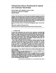
2. RDF PRELIMINARIES Resource Description Framework (RDF) is an assertional language to express propositions using formal vocabularies [50]. The main advantage of RDF is the generality of its design which allows expressing propositions about any topic if the right vocabulary is available. Particularly, RDF allows decomposing knowledge of any kind into concise, atomic parts and then establishing relationships among those parts in the form of vertices and edges of a directed graph. The abstract syntax of RDF [3] defines an RDF graph as a collection of triples, where each one expresses an assertion in the form of a 3-tuple and containing a subject, a predicate, and an object. Figure 1 shows an example, where two basic geographical facts about Arizona State University are expressed as triples. In general, a triple expresses a fact (knowledge assertion) between two real-world entities described by the subject and object. A set of RDF triples can, then, be seen as the logical conjunction of the assertions of its underlying triples; a set of RDF statements can also be often viewed as a graph: the subject of a triple represents vertices in the RDF graph whereas the predicate represents the edge connecting them. The entities represented by the nodes in an RDF graph are uniquely identified using uniform resource identifier (URI) references [51], literals, and blank nodes, which are a special kind of node that is neither a URI reference nor Subject Arizona State University Arizona State University Fig. 1.
Information represented as triples
14
Predicate latitude longitude
Object 33.42 -111.93
33.42 -111.93 Fig. 2.
RDF knowledge base in Figure 1 serialized in RDF/XML format
@prefix geo: . geo:lat "33.42". geo:long "-111.93".
(b) Turtle serialization Fig. 3.
RDF knowledge base in Figure 1 serialized in Turtle format
a literal and that is used to uniquely identify a node in the graph without having a specific name; whereas predicates (graph edges) are identified using only URI references. Note that the RDF model is inherently abstract; for this reason, the W3C also introduced a standard, referred to as RDF/XML [52], for its serialization. In addition to this, there are two other non-standard formats that are widely used due to their ease and readability: Notation 3 (N3) [53] and its extension Turtle [54]. Figures 2 and 3 show the serialized version of the triples of Figure 1 in RDF/XML Turtle format respectively.
15
2.1. SPARQL Preliminaries SPARQL is the query language introduced by the World Wide Web Consortium (W3C) to query RDF information. Its purpose is to express queries in the form of graph patterns that match and retrieve subgraphs from an RDF graph. SPARQL introduces the concept of variable to specify any node in the graph; and the concept of triple pattern which is a construct identical to an RDF triple but that may contain a variable in the place of the subject, predicate, or object [6]. The basic unit of a SPARQL query is the Basic Graph Pattern (BGP) which is defined as a set of triple patterns. Similarly, the set of all BGPs in a query, separated by curly brackets is called a group graph pattern. In general, the purpose of a SPARQL query is to find subgraphs of the underlying RDF graph that match a BGP. In other words, a subgraph s is a valid match for a BGP b if after substituting the variables and blank nodes of b with RDF terms of s, both b and s are equal. The subgraphs resulting from substituting the variables and blank nodes of b with RDF terms are called a solution mapping and an RDF instance mapping respectively. In addition, the matching subgraphs for b form a multiset of pattern instance mappings, which are defined as the combination of a solution mapping and an RDF instance mapping. Finally, these three components define a solution µ for a BGP b over and RDF graph G as the existence of a pattern 16
instance mapping P such that P (b) is a subgraph of G and P is restricted by µ to the variables in b [6]. 2.2. SPARQL Query Processing The steps to process a SPARQL query include parsing, algebra generation, and evaluation [55]. The parser converts a query string into an abstract syntax tree (AST) and the AST is further processed to obtain a tree-like expression containing algebraic operators. After this expression is built, the query engine proceeds with its evaluation starting with the operators at the leaves of the tree. The basic set of algebra operators include project to select only a subset of the variables bound in a solution mapping; bgp to evaluate basic graph patterns; filter to constrain the matches for a BGP to conditions applied to their labels or numeric values; join, union, and leftjoin to perform conjunctions, disjunctions, and optional matching of BGPs respectively; and order by, distinct, reduced, and slice, to modify the sequence of results returned by the previous operators [6]. The evaluation of a BGP to find matching subgraphs comprises the join of the matches for its individual triple patterns. In particular, the algebra operator bgp performs the join of triple patterns belonging to the same basic graph pattern, whereas the join operator performs joins at the group graph pattern level; i.e., between basic graph patterns if there is more than one. However, despite their differences, both join operations operate under the same principle of solution mapping compatibility, which states that two solution 17
Fig. 4.
Sample RDF graph
SELECT ?state WHERE { {?spec1 :type :bird . ?spec1 :location ?state} {?spec2 :type :reptile . ?spec2 :location :?state} } Fig. 5.
A SPARQL query over the RDF graph in Figure 4
mappings µ1 and µ2 are compatible if all their common variables are bound to the same values in both of them [6]. Consider the RDF graph in Figure 4 containing information about three animal species and their respective locations. The SPARQL query in Figure 5, containing a group graph pattern with two BGPs, searches for the states that have both birds and reptiles. After the parsing process, the generated algebra expression is evaluated by the query engine starting with the operators at the lowest levels of the tree, i.e. the BGP operators. Figure 6 shows the partial results (shown over the outgoing arrows) for each BGP operator and the final joined result. Note that
18
Fig. 6.
Algebra tree for the SPARQL query in Figure 5
only the solution mappings corresponding to Roadrunner and Rattle snake are joined by the join operator as they are compatible regarding their common variable ?state.
19
3. WEIGHTED RDF MODEL In this section, we present the proposed extension to the RDF model. The weighted extension of the RDF model simply associates to each of the underlying components of the RDF model, i.e. triples, an application-specific numeric value representing a measure of desirability or lack thereof. Weighted Triple. A weighted triple tw is a 4-tuple composed of Subject (S), Predicate (P), Object (O), and a real value w between 0 and 1 representing the weight of the assertion made by the triple SPO. Weighted RDF Graph. A weighted RDF graph Gw is defined as a set of weighted triples. In this thesis, triples with weights are represented as quadruples, where the final value of the quadruple is the weight of the triple , instead of relying on reification – which could be used to associate weights to the triples indirectly through reified statements. The reason why we treat weights as first class knowledge attributes (as opposed to treating them as any other application specific attribute, which can be specified using reification statements) is that we would like the underlying engine to easily recognize and leverage these weights in indexing the knowledge statement (Section 5.3.1) and processing users’ ranked queries over the weighted graphs (Chapter 5). Note that this is not a strict requirement in that the same effect can also be achieved using a special reification statement recognized by the underlying indexing and query processing engine.
20
@prefix biol: . @prefix : . :Chondrichthyes :Chondrichthyes :Chondrichthyes :Chondrichthyes :Holocephali :Elasmobranchii :Elasmobranchii :Elasmobranchii
biol:subclass biol:subclass biol:subclass biol:subclass biol:subclass biol:subclass biol:subclass biol:subclass
:Elasmobranchii :Holocephali :Dusky Shark :White Shark :Chimaeriformes :Chondrichthyes :White shark :Basking Shark
0.10 0.01 0.05 0.30 0.10 0.50 0.90 0.10
. . . . . . . .
Fig. 7. Extended, Turtle-based, representation of a sample weighted RDF knowledge base (adapted from [1, 2])
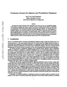
Fig. 8.
A sample weighted RDF Graph (adapted from [1, 2]
Figure 7 shows a set of weighted RDF triples, in Turtle format [54], containing RDF information adapted from the weighted graph representing the integration of two shark taxonomies used in [1, 2]. In this example, the weight value associated with each edge (RDF triple) represents the amount of disagreement on the corresponding assertion. The weight value extending the original Turtle format is shown in bold along with each triple. Similarly, the weighted RDF graph for this triple set is shown in Figure 8. 21
3.1. Query Language Extensions As we discussed in the Introduction, we propose the following extensions to the common RDF query language: • an extension to the syntax of Triple Patterns to include an optional element (variable or literal) that reflects the weight associated to the matches of the triple pattern. • path predicates to allow queries to express relationships between subjects and objects with one or more predicates between them (similar to the ancestor-descendant (//) axis of XPath [15]), • a “SELECT @” clause that enables outputting of each matching result in the form of a set of RDF triples, and • a “RANK” clause to state that the user is interested in only the top-k solutions (where k is user specified) for a query pattern based on the weights of the statements. In this section, we describe these extensions, building on the SPARQL query language [6]. 3.1.1. Extended Triple Patterns An extension to the syntax of Triple Patterns is proposed to include an optional element, variable or literal, to reflect the weight associated to the matching results of the given pattern. In particular, the new element is introduced to 22
SELECT ?o ?w WHERE { :Chondrichthyes ?p ?o ?w . FILTER (?w > 0.01)} Fig. 9. Sample query containing a triple pattern extended by a new variable (variable ?w) to associate the weight of the returned matches
comply with the extension to the underlying RDF model, i.e. in addition to matching the subject, predicate, and object of a triple, an extended triple pattern allows matching its associated weight. This means that the additional element can be used in the same way as the other elements in the triple pattern, i.e. if it is a bound variable or a literal, it will participate in the matching process as an extra constraint; on the other hand, if it is an unbound variable, it will be bound to the associated weight of each result matching the triple pattern. In addition, as a variable, it can be used freely by other patterns or operators, such as filter or select, within the query. Figure 9 presents a sample query to retrieve the objects of the triples that contain :Chondrichthyes as a subject and a weight greater than 0.01. 3.1.2. Path Query Predicates We propose a novel query predicate to represent multi-edge relationships between two nodes in an RDF graph; the predicate matches one or more edges irrespective of the labels of the edges or vertices on the path. The predicate can be extended to impose additional constraints over the multi-edge relationships represented by it. In particular, the syntax
23
SELECT * WHERE { :Chondrichthyes ?s }
(a) SELECT * WHERE { :Chondrichthyes ?s }
(b) SELECT * WHERE { :Chondrichthyes ?s }
(c) Fig. 10. Sample extended SPARQL queries containing a path predicate which allows multiple matching edges with (a) no restrictions (b) a restriction (subclass) on the edge label and (c) two additional restrictions on the edge weights to specify lower and upper limits (prefixes omitted)
supports three optional parameters which can be used to constrain the edges of the relationship to have a specific label, and to constrain the lower and the upper limits to the aggregated weight of each matching result returned by the predicate. These parameters are completely independent from each other; therefore a given predicate may contain none, one, two, or all of them. Note that putting path constraints along with the path predicate allows the path search algorithm (Section 5.1) to recover only those paths that comply with the constraints while avoiding unnecessary ones that need to be filtered later. Figure 10 presents three sample queries, over the RDF dataset from Figure 8 to retrieve all the nodes reachable from :Chondrichthyes with a path containing one or more edges with (a) no restrictions on the paths returned, 24
SELECT ?s WHERE { ?s :Holocephali . ?s ?p1 :Dusky_Shark . ?s ?p2 :White_Shark . } Fig. 11. A sample query where path predicates are used in conjunction with other SPARQL constructs
(b) with a restriction (subclass) on the edge labels and (c) with an additional restriction on the lower and upper limits of the edge weights. Path predicates can be used like any regular query predicate, i.e. the subject can be an IRI or a variable and the object can be either an IRI, a literal, or a variable. Naturally, the new path predicate can be used in conjunction with other query patterns, which in turn can contain other path predicates or simple regular SPO patterns, and SPARQL clauses (see Figure 11 for an example). 3.1.3. “SELECT @” Clause As described in Section 2.1, the “SELECT” clause of SPARQL allows the user select the variables that will be included in the output. For example, in Figure 11, the user states the she is interested in the values of the ?s variable, whereas the values of the ?p1 and ?p2 variables are ignored. In contrast, when the “SELECT *” clause in Figure 10 is used, the matching values for all the variables in the query are included in the result.
25
SELECT @ WHERE { :Chondrichthyes ?o . FILTER regex(str(?o) ,"White_Shark", "i") }
(a) A sample “SELECT @” query (1)[0.30] :Chondrichthyes :White_Shark (2)[1.00000] :Chondrichthyes :Elasmobranchii :White_Shark
biol:subclass
:White_Shark ‘‘?o’’
0.30 . 0.0 .
biol:subclass biol:subclass
:Elasmobranchii :White_Shark ‘‘?o’’
0.10 . 0.90 . 0.0 .
(b) Result based on the RDF graph in Figure 8 Fig. 12. (a) A sample “SELECT @” query and (b) the corresponding set of results; each of which is a matching path described in the form of a set of RDF triples (since each triple has a weight, each result is also associated a weight displayed within square brackets – in this example, the overall score of a result is the sum of the corresponding triple scores)
One difficulty with the standard “SELECT” and “SELECT *” clauses is that they allow the query to return only named variables. However, as shown in Figure 10, the path predicate, , matches entire paths, consisting of one or more edges; consequently, only the end points of these paths can be associated with named variables that can be returned to the user. In order to deal with this shortcoming of the standard SPARQL, the “SELECT @” clause is introduced, which outputs the entire matching result subgraph in the form of a (serialized) RDF graph; any variables on this graph are annotated through a special “isVar” triple as shown in Figure 12. Therefore, the user can ask further queries on this graph to explore any edges or nodes that have not been explicitly enumerated in the query specification. 26
SELECT * WHERE { {:Chondrichthyes ?o1 ?w1 . :Elasmobranchii ?o2 . }SCORE IN ?w } Fig. 13.
A sample query showing the use of the SCORE clause
3.1.4. “SCORE” Clause The basic unit of a SPARQL query is the Basic Graph Pattern (BGP) (Section 2.1)which is defined as a set of triple patterns. Alike the extension for triple patterns, we propose the SCORE clause to associate the score (weight) of a solution for a BGP as a whole. The SCORE clause takes as a parameter a variable name which will be included in the set of query variables and bound to the weight of each resulting match for the BGP to which the clause belongs. Figure 13 shows a sample query using the SCORE clause. Note that the variable ?w introduced by the new clause reflects the aggregated weight of every resulting match for the BGP of the query; whereas the variable ?w1 reflects the weight of the matches only for the triple pattern associated with it. In addition, the variable included by the SCORE clause can be used like any other variable in the query, i.e. it can be compared, sorted, and filtered. Finally, the scope of the new clause is the same as that from FILTER, this means that it can be applied to different parts of a query as long as these parts belong to different group patterns.
27
SELECT ?s ?w WHERE { {?s :Holocephali . ?s :Dusky_Shark . ?s ?p :White_Shark . RANK 10 }SCORE IN ?w } Fig. 14.
An example query showing the use of the RANK clause
3.1.5. “RANK” Clause The queries presented so far return all possible matches for the given query patterns. However, the weight information associated with the underlying RDF graph and triples allows ranking the results returned by a query and limiting their number based on a k given by the user. To support this, we propose a RANK clause which takes as a parameter an integer number k greater than or equal to 1, indicating the desired number of top results. Figure 14 shows the use of the RANK clause applied to our previous query to return the top-10 common classes with the lowest amount of disagreement regarding the underlying taxonomy. Note that the scope of RANK is the same as that of the SCORE clause. Additionally, the scope of the RANK clause is the group pattern in which it occurs, in a similar way to the FILTER clause of SPARQL (see Section 5.2.2 in [6]). This means that the RANK clause can be applied to different parts of a query as long as these parts belong to different group patterns; i.e., they are separated by curly brackets. For instance, the query in Figure 15 retrieves the top-5 results of the join of
28
SELECT ?o ?w WHERE { {{:Chondrichthyes ?o RANK 3} {:Elasmobranchii ?o RANK 3} RANK 5 }SCORE IN ?w } Fig. 15. A sample query illustrating the use of multiple RANK statements in a single query
two different group patterns, which in turn are limited to 3 results each. Note, however, that queries of this type must be used carefully as the underlying join operator may need more than 3 results from each side to return the top 5 results for the whole query (this will be discussed in detail in Section 5.2).
29
4. EXTENDED QUERY OPERATORS Extensions of the SPARQL query language with extended triple patterns, path predicates and the new clauses as described in the previous section necessitate (a) formal definitions of the semantics of the underlying algebra, (b) implementation of physical operators to support these extensions, and (c) a reconsideration of the SPARQL query processing strategies. These aspects are explained in detail in this and the following sections. 4.1. Extended Graph Pattern Matching As described in Section 2.1, the unit of representation in SPARQL is the basic graph pattern (BGP) which is expressed as a set of RDF triples that form a graph pattern and that may contain variables as the subjects, predicates, or objects. The BGP is matched against an RDF graph to obtain a solution subgraph whose nodes are bound to the variables of the BGP. A solution for a BGP in SPARQL comprises a subgraph, which maps the BGP against an RDF graph, along with solution and instance mappings binding variables to the nodes of the subgraph. In this section, following [6], we extend the definitions of triple pattern and solution mapping, and define a solution over a weighted RDF graph. Extended Triple Pattern.
Let RDF-PP be the set {},
an Extended Triple Pattern is a member of the set (RDF-T ∪ V ) × (I ∪ V ∪ RDF-PP) × (RDF-T ∪ V ) Note that the definition of Extended Triple Pattern includes path query patterns as it uses the special path predicate . Similarly, path query 30
predicates are defined as a regular IRI predicate; therefore the notion of solution mapping as a partial function V →T still applies. However, solution mappings over RDF graphs must have a weight value associated with them. This calls for the definition of weighted solution mapping and solution over a weighted RDF graph1 . Weighted Solution Mapping. A weighted solution mapping µw is a pair (µ, w) composed of a solution mapping µ and a real value w representing its weight. The cardinality of µw in a multiset Ωw of weighted solution mappings is expressed as cardΩw (µw ). As defined in [6], a solution mapping that is a solution for a BGP represents a solution subgraph. This implies that the weight associated with a weighted solution mapping represents the aggregation of the weights of the triples in the subgraph. Specifically, we define weight aggregation function. Weight Aggregation Function.
A weight aggregation function
aggW(µw ) is a function that determines the aggregated weight of a weighted solution mapping µw by applying an aggregation function to the weights of the underlying subgraph of µw . Note that the aggregation function applied to the weights of the triples of the underlying subgraph can be either sum, min, max, average, or product. Solution over a weighted RDF graph. Let Gw be a weighted RDF graph, and let bgp be a Basic Graph Pattern. A solution over Gw for bgp is a 1 Similar
to the definitions presented in [4]
31
SELECT * WHERE { :Chondrichthyes ?o ?w }
(a) ?o -> :Dusky_Shark ?w -> 0.05 ?o -> :Chimaeriformes ?w -> 0.11 ?o -> :White_Shark ?w -> 0.30
(b)
(c) Fig. 16. Sample path query (a) over the graph in Figure 8 showing (b) the bound variables of its solution mappings, and (c) the underlying graph corresponding to the second solution mapping
weighted solution mapping µw that combines a solution mapping µ from variables to nodes, an instance mapping σ from blank nodes to nodes, a weighted subgraph gw of Gw defined as µ(σ(bgp)), and a weight w given by a Weight Aggregation Function aggW(µw ). The cardinality cardΩw (µw ) for each µ is defined as the number of distinct RDF instance mappings σ such that µ(σ(bgp)) is a subgraph of Gw . Figures 16a and 16b show a query over the weighted RDF graph from Figure 8 with its respective weighted solution mappings presented in nondecreasing order of their weight. The bindings are shown as arrows going from the variable to the bound value. Similarly, Figure 16c presents the subgraph associated with the weighted solution mapping corresponding to [?o
32
-> :Chimaeriformes ?w -> 0.11] and that is used to compute its weight. Note that in this case the aggregation function used to compute the weight is sum. Alternative aggregation functions like min, max, average, and product would give the solution mapping a different weight (0.01, 0.10, 0.055, and 0.001 respectively) and would potentially change the order of the final results. In addition to simple BGP matching, SPARQL provides operators to allow expressing more complex queries using one or more group graph patterns [6]. They operate over multisets of solution mappings to perform operations like Join, Union, Project, Filter, Order, and Distinct. However, the SPARQL specification does not consider weight values associated with solution mappings. Plus, the new clauses SCORE and RANK need to work with operators that consider this associated weight. Therefore, these operators need to be redefined so they can use the associated weight value when creating new solution mappings. SPARQL operators create new solution mappings by merging two solution mappings if they are compatible 2 . The function merge applied to two solution mappings µ1 and µ2 is defined as µ1 ∪ µ1 . In presence of Weighted Solution Mappings, this function needs to be extended to perform the aggregation of the weight values associated with them. Weight Merge Function. A weight merge function mergeW(µw1 , µw2 ) is a function that determines the aggregated weight of two weighted solution 2 Two
solution mappings are compatible if for every variable v in both mappings, v is bound to the same value
33
mappings µw1 and µw2 by applying a Weight Aggregation Function aggW to the weights of the subgraph resulting from merge (µw1 , µw2 ). Next, we present the algebra definitions of the operators for our proposed clauses, as well as the redefinition of the existing SPARQL in order to add the support for the processing of weighted solutions. Our algebra definitions follow those presented in the SPARQL specification. Weighted Join Operator.
Let Ωw1 and Ωw2 be two multisets of
weighted solution mappings, the result of the join operator is a multiset of weighted solution mappings defined as Join(Ωw1 , Ωw2 ) = { (merge(µ1 , µ2 ), mergeW (µw1 , µw2 )) | µw1 ∈ Ωw1 ∧ µw2 ∈ Ωw2 ∧ µ1 and µ2 are compatible} with
cardJoin(Ωw1 ,Ωw2 ) (µw ) =
P µw1 ∈ Ωw1 µw2 ∈ Ωw2
cardΩw1 (µw1 ) ∗cardΩw2 (µw2 ) if µw = (µ, w) with w = mergeW (µw1 , µw2 ) µ = merge(µ1 , µ2 ) where µwi = (µi , wi ) 0 else
Note that although Ωw1 and Ωw2 are defined as multisets, their weighted solution mappings are ordered (ranked) in non-decreasing order of their weight. This implies that the Weighted Join Operator has to return results in a ranked 34
manner. For this, the query processor engine should make use of well-known ranked-join algorithms [43, 56–58] to perform the join operation efficiently. However, there are cases in which the use of this type of algorithms is not possible. For instance, if the aggregation function being used is sum and the subgraphs of the two solution mappings have triples (edges) in common, the weights of the common edges may need to be counted only once. This situation violates the monotonicity of the results required by common ranked-join algorithms. In this case, the query processor engine should use a more appropriate algorithm such as HR-Join [2]. We leave the details of join processing to Section 5.2. In order to have access to the weight value of a weighted solution mapping µw the proposed SCORE clause adds its parameter variable, bound to the weight of µw , to the set of variable bindings of µw . Score operator. Let Ωw be a multiset of weighted solution mappings; let v be a query variable; a Score operator is defined as score(Ωw , v) = {(µsw , w) | (µ, w) ∈ Ωw ∧ µsw = µ ∪ (v, w)} cardscore(Ωw ,v) (µw ) = cardΩw (µw ) Similarly, the RANK clause acts as a wrapping operator for any SPARQL operator that returns a multiset of weighted solution mappings. This gives RANK the ability to control the number of results that must be returned by the nested operator, which is specified by a positive integer k sent as a parameter. Rank operator. Let Ωw be a multiset of weighted solution mappings; 35
let k be a positive integer; a Rank operator returns a multiset Ωwr created by obtaining at most k elements from Ωw and preserving their order and cardinality. If the number of elements in Ωw is less than or equal to k, Ωw and Ωwr are the same. As described in Section 3.1.3, the SELECT @ clause returns the serialized RDF form of the subgraph of each solution mapping matching a BGP. To support this functionality we define the SelectAt operator SelectAt operator. Let Ψw be a sequence of weighted solution mappings; let x be the set of variables and blank nodes of the BGP from which Ψw is obtained; let σ be the RDF instance mapping of the blank nodes of BGP in each solution mapping of Ψw . The result of a SelectAt operator is a sequence defined as SelectAt (Ψw ) = {(µsα , w) | (µw , w) ∈ Ψw ∧ µsα = µ (σ (x))} cardSelectAt(Ψw ,w) (µw ) = cardΨw (µw ) The order of SelectAt (Ψw ) must preserve the order given by orderBy. Filter operator. Let Ωw be a multiset of weighted solution mappings and exp be an expression (as defined in [6], Section 3). The result of a Filter operator is a multiset ofweighted solution mappings defined as µw | µw = (µ, w) ∈ Ωw ∧ exp (µ) is an f ilter (exp, Ωw ) = expression that has an ef f ective boolean value of true cardf ilter(exp,Ωw ) (µw ) = cardΩw (µw )
36
Union operator. Let Ωw1 and Ωw2 be two multisets of weighted solution mappings. The result of a Union operator is a multiset of weighted solution mappings defined as: union (Ωw1 , Ωw2 ) = {µw | µw ∈ Ωw1 or µw ∈ Ωw2 } cardunion(Ωw
1 ,Ωw2
) (µw ) = cardw1 (µw ) + cardw2 (µw )
Note that, similar to the Join operator, the query processor engine needs to return ranked solution mappings resulting from the union of Ωw1 and Ωw2 . OrderBy operator. Let Ψw a sequence of weighted solution mappings; let cond be a condition (defined in [6], Section 9.1), the result of an OrderBy operator is a sequence defined as µw | µw ∈ Ψw and the sequence orderBy (Ψw , cond) = satisf ies the ordering condition cardorderBy(Ψw ,cond) (µw ) = cardΨw (µw ) Project operator.Let Ψw be a sequence of weighted solution mappings and PV a set of query variables. The result of a Project operator is a sequence defined as: For mapping µw , write Proj(µw ,PV) to be the restriction of µw to the variables in PV. project (Ψw , P V ) = [P roj (µw , P V ) | µw ∈ Ψw ] cardproject(Ψw ,P V ) (µw ) = cardΨw (µw ) The order of project (Ψw , P V ) must preserve the order given by the orderBy operator.
37
Distinct operator. Let Ωw be a sequence of weighted solution mappings. The result of a Distinct operator is a sequence defined as distinct (Ψw ) = [µw | µw ∈ Ωw ] carddistinct(Ψw ) (µw ) = 1
38
5. EXTENDED QUERY PROCESSING ENGINE In this chapter, the details of the query processing engine required to parse, generate, optimize, and evaluate a SPARQL query containing the new and redefined operators proposed in the previous chapter are presented. Also, we describe the processing of path predicates and how they are used in conjunction with the new clauses and join processing to evaluate ranked queries more efficiently. The indexing approach to solve path queries more effectively is also described. 5.1. Shortest paths In section 3.1.2 the functionality of our proposed path predicate was briefly described. In this section, a description of the operator used by the query engine to evaluate path query patterns is presented. In particular, the query engine is extended to return solution mappings that match both triple and path patterns. Additionally, the extension to support ranked top-k queries motivates the use of algorithms that allow finding these structures in a very efficient way. For this, a version of Yen’s algorithm [59] presented in [16] which returns the k-shortest simple paths between two given nodes is used and it was chosen due to its optimal nature. The evaluation of a path pattern starts by identifying the type of the start and end nodes of the path pattern. For instance, if both are non-variables, Yen’s algorithm is invoked directly on them; otherwise, variable nodes are replaced by a temporary node connecting, through predicates, all the nodes that
39
SELECT * WHERE { ?s :White_Shark . RANK 1} Fig. 17.
Path query to find the top-1 class for which :White Shark is a subclass
are reachable from (or can reach) the non-variable node in the path pattern 1 . Reachable (or reaching) nodes are found by means of a reachability index (See section 5.3). Note that k-shortest paths algorithms require that both start and end nodes be specific nodes in the graph; however, this is not the case for variable nodes as they may represent any node in the graph. After the variables of a path pattern have been processed, this is ready to be evaluated by the query engine using Yen’s algorithm. In particular, the query engine associates the algorithm with a path operator which implements an iterator to return results in a pull-based manner 2 , i.e. paths are produced on-demand based on the requirements of the operator using the path operator. Each retrieved path is then processed to remove the temporary node and its edge and to create a weighted solution mapping by binding their nodes, predicates (edges), and weight to variables in the path pattern. Finally, once the path iterator is not required to return more results, the temporary nodes along with its edges are removed from the graph. 1 This is done by adding temporary weighted triples with weight 0 to the underlying RDF graph 2 This
contrasts with [2] in which Yen’s algorithm is used with a push-based approach returning paths permanently until instructed to stop
40
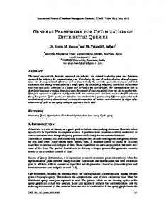
Fig. 18. Graph from Figure 8 modified to include a temporary node that links the nodes that can reach the node :White Shark
Consider the query in Figure 17 which retrieves the top-1 class for which :White Shark is a subclass. As the subject of the path pattern is a variable, it needs to be replaced by a temporary node linking the nodes that can reach :White Shark, i.e. :Chondrichthyes and :Elasmobranchii. Figure 18 shows the modified version of the graph in Figure 8 (the temporary node tmpNode is shown in grey). After this addition, the query engine executes Yen’s algorithm to find the top-k paths between tmpNode and :White Shark. As expected, the shortest path between these two nodes is the one connecting tmpNode→:Chondrichthyes →:White Shark with weight 0.30. Once this path is found, tmpNode and its temporary edges are removed from the path and graph, and the path is returned.
41
5.1.1. Enhanced query processing using path operators A path operator is not considered an independent algebra operator as it is never evaluated in isolation but always within the context of a BGP operator, like any regular triple pattern. Therefore the BGP operator may greatly benefit from using a path operator to evaluate its triple patterns as a whole instead of considering them independently. Specifically, the use of path operators is not limited only to the evaluation of single path query expressions, i.e. a single expression containing one path predicate and one start and end node, but it can also be extended to the evaluation of more complex queries that contain more than one path (or triple) pattern and that can be seen as an extended path pattern with intermediate nodes. For example, consider the query in Figure 19 which asks for the top-5 intermediate subclasses connecting the class :Elasmobranchii and the subclass :Chimaeriformes. The regular approach to solve a query like this is to apply a path operator to each path pattern and then perform the ranked join of the results. Alternatively, the query engine can treat this query as a single path pattern from :Elasmobranchii to :Chimaeriformes with an intermediate node ?o and use a single path operator to return ranked results without requiring a join operator. In this case, the path operator also needs to consider intermediate nodes in the query pattern in order to a) validate the lengths of the retrieved paths, and b) perform the appropriate variable bindings. 42
SELECT * WHERE { :Elasmobranchii ?o . ?o :Chimaeriformes RANK 5} Fig. 19.
Query composed of two simple path patterns
In our example, the length validation considers only paths with at least two edges (one intermediate node), and the binding process associates ?o with :Chondrichthyes and :Holocephali (See Figure 8) which will have the same aggregated weight as they occur in the same (and only) path from :Elasmobranchii to :Chimaeriformes. 5.2. HR-Join operator The evaluation of a BGP operator involves the evaluation of its composing triple and path patterns and then the join of the solution mappings produced by them. Similarly, join operations are also performed at a higher level, i.e. when joining solution mappings produced by two or more BGPs (group graph patterns). In this section, we present the details of the extension to the SPARQL join operator to work over ranked inputs of weighted solution mappings. Specifically, as mentioned in previous sections, a join operator working with ranked input streams of weighted solution mappings also needs to return a ranked sequence of joined weighted solution mappings either by using conventional ranked-join algorithms [43, 56–58], if the aggregation function being used is monotonic, or alternative join algorithms such as [2] otherwise.
43
The non-monotonicity problem occurs during the aggregation of the weights of two solution mappings whose subgraphs have overlapping edges. In particular, during this computation, the weight of the edges (triples) of each subgraph is processed by a Weight Merge Function to assign a weight to the results of the join operation. Depending on specific application requirements, this function may process overlapping edges, i.e. edges that are common to both subgraphs, only once or twice. When common edges are processed only once, aggregation functions like sum and product may affect the monotonicity of the produced results. For instance, assume we use the function sum 3
, then the aggregated weight of two subgraphs with high individual weights
and many overlapping edges may be lower than that of two subgraphs with lower individual weights but with zero overlapping edges [2], inducing this way non-monotonicity in the aggregation function. On the other hand, when overlapping edges are treated independently, then the join operator behaves like a usual ranked-join algorithm as the aggregation function is always monotonic. Note that for aggregation functions like min and max, monotonicity holds even if overlapping edges are considered only once. Next, we present the details of the join operator considering its aggregation function as non-monotonic. For the evaluation of the join operator using a non-monotonic aggregation function we extend the functionality of the HR-Join operator, presented in [2]. 3 For
the case of product note that a . b = c is equivalent to log(a) + log(b) =
log(c)
44
In general, this extension allows the operator to (a) work with general structures not limited to twigs, (b) access its input streams more efficiently using a pull-based approach, (c) match two sub-results in one or more nodes not limited to a root node, (d) be fully compatible with other SPARQL algebra operators occurring in an algebra expression. The evaluation of the extended HR-Join operator follows, in a general way, the process thoroughly described in [2]. In general, the input streams to the join operator are managed by horizon valves to control the availability of data. Then, the (Symmetric Hash) join operation pulls sub-results from each valve in a round-robin manner. Sub-results in one valve are compared against those from the other valve to find possible matches based on their root nodes. Once a match is found, it is passed to the Result Sieve whose function is to return a cost-ranked stream of results while dealing with the non-monotonicity of its input stream. The extension to this evaluation process involves the implementation of the HR-Join as a cost-ranked iterator of weighted solution mappings and the association of the horizon valves with other cost-ranked iterators, such as path or other join operators, in order to seamlessly include the new operator in a SPARQL algebra tree generated from a query. As described in Section 5.1, the association of the horizon valves with iterators improves the access to the input streams as sub-results are produced on a pull-based instead of a push-based manner. 45
SELECT ?s ?w WHERE { {?s :Chimaeriformes ?w1 . ?s :Dusky_Shark ?w2 . RANK 5 }SCORE IN ?w } Fig. 20. Sample query to find the top-5 common classes for the subclasses :Chimaeriformes and :Dusky Shark
Another important aspect of our extension is the ability of the HR-Join operator to produce results that are not limited to twigs, and to match subresults based on several nodes rather than on one root node. This extension involves the use of mapping compatibility introduced in Section 2.2. In particular, when a sub-result (weighted solution mapping) in one valve has to be compared to those in the other valve, this operation is reduced to a verification of mapping compatibility between sub-results, i.e. the existence of common variables bound to the same values in all of them. Consider the query in Figure 20 to find the top-5 common classes for the subclasses :Chimaeriformes and :Dusky Shark. The BGP evaluation involves the join of the two path patterns which are associated to path operators. For this example, we assume that the join operator uses sum as the weight aggregation function and it counts overlapping edges only once. Internally, the join operator associates each path operator with a horizon valve. As described in [2], the join operator pulls paths from each valve in a round-robin manner. Every time a valve pulls a path, it is compared to those already pulled in the
46
(a) Fig. 21.
(b)
HR-Join stages for query in Figure 20
other valve. Figure 21(a) shows the query algebra tree and a snapshot of the intermediate solution mappings (paths) when both valves have pulled two and one path respectively. After the left valve pulls the second solution mapping, it finds a match with the first solution mapping from the right valve as they are compatible. However, it is not output by the join operator (shown in grey) until it verifies that the maximum score in each valve is greater than the score of the result just found or that both valves have finished their outputs. In Figure 21(b) the left valve finds another match with the second solution mapping from the right. Note that the solution mappings joined to create the second result have one overlapping edge, :Elasmobranchii→:Chondrichthyes, which is counted only once by the join operator. For this reason, the aggregated weight of the second result is 0.66 instead of 1.16. Finally, since both valves have finished their outputs, both results are output by the join operator.
47
5.3. Indexing In this section, the details of the index structures used to support the extensions described in previous sections are presented. Specifically, the extension to the index structures of Jena TDB [8] is described; along with the details of a reachability and graph proximity indices. The first one is used during the processing of path operators to replace variable nodes with reaching or reachable nodes; whereas, the second one is used for query optimization (Chapter 6). 5.3.1. Weight Aware Indexing The RDF storage framework of Jena, TDB [8], provides three composite indices, subject-predicate-object (SPO), predicate-object-subject (POS), and object-subject-predicate (OSP) for efficient execution of queries on disk-resident RDF graphs. In order to avoid any full table scans when executing a query, we extend the indexing scheme of TDB in such a way that results can be returned in non-increasing order of their weight no matter what literals are available in the query pattern. Thus, our extended indexing scheme contains nine composite index structures, SWPO, SPWO, SPOW, PWOS, POWS, POSW, OWSP, OSWP, and OSPW, where W denotes the weight of the triples. In addition, alike the original SPO fields, the weight field is internally represented as an inline 64 bit node identifier [8]. The choice to represent it this way has the double benefit of (a) avoiding expensive conversions from Node to NodeID, and vice versa, and (b) allowing the order of triples according to their weight.
48
5.3.2. Reachability Index As explained in Section 5.1, a path pattern may contain variable nodes as its start or end nodes. However, the underlying Yen’s algorithm used to find paths needs specific node labels to initialize its search. In addition, a variable node as a start or end node in a path pattern indicates a path from or to any node in the graph. For this reason, in order to reduce the path search time, it is necessary to reduce the search space of Yen’s algorithm to a reachability neighborhood, i.e those nodes that are reachable or can reach the non-variable node in the path pattern. The retrieval of the reachability neighborhood of a node needs to be processed during query evaluation. This requirement discards online methods to recover reachability information; therefore we make use of an all-pairs reachability index to recover this information quickly without affecting the performance of the query evaluation. The high cost of computing an all-pairs reachability index, O(V 3 ), is acceptable as this index is generated offline along with the generation of the extended TDB database described in the previous section. 5.3.3. Proximity Index The proposed extensions include an optimization strategy (See Chapter 6) to improve the execution time of top-k queries. This strategy is based on statistical information about a weighted RDF graph regarding graph proximity [27, 28]. Essentially, graph proximity is a measure that summarizes the 49
relationships between any two nodes in the graph such as the number, length, and weight of the paths between two nodes. In other words, two nodes are closer to each other if the paths connecting them are large in number, short in length, or have a low weight. In this thesis, a variant of the reachability computation algorithm presented in [28] is used. In general, this algorithm uses a proximity definition based on properties of random walks [60–62] to characterize node relationships based on the paths connecting them. In order to generalize the use of random walks to directed graphs, the algorithm introduces the concept of escape probability between two nodes i and j, which is defined as the probability that a random particle starting from i visits j before it returns to i. Finally, the algorithm adds parameters to reflect noise that may distract the particle from reaching its goal, and to reduce the asymmetry in the graph connectivity induced by its directed edges. Our proposed optimization strategy uses all-pairs proximity information computed over the underlying RDF graph. Similar to reachability neighborhoods, all-pairs proximity information is used during query processing time; therefore, for better performance, it is computed offline and stored as an additional index. As an example of this, the proximity indices created for the experimental datasets presented in Chapter 7 had a creation time of approximately three hours.
50
6. OPTIMIZATION 6.1. Preliminaries The evaluation of a basic graph pattern involves the join of its component triple and path patterns. Specifically, the query engine creates a query plan which is represented as a rooted binary tree in which the leaf nodes are triple or path patterns and the non-leaf nodes are join operators. As described in Section 5.2, to perform join operations the extended query engine uses an extension of the HR-Join operator proposed in [2] in order to deal with the potential non-monotonicity of the sub-results produced by the join operations. Essentially, this operator is based on a symmetric hash join which pulls subresults from each of the input streams being joined in a round-robin manner. For this, the operator keeps a map associated with each input stream to keep record of of every single sub-result retrieved so they can be compared to those from the other input to find potential matches. When a match is found, it is stored in a special structure for further processing. For this, the operator maintains a priority queue of candidate results which outputs one result at a time when the conditions to avoid non-monotonicity are met. This process is repeated every time the operator is required to return a result. Note that, similarly to classic rank-join operators, the HR-Join operator is optimized to return ranked results without having to access all the subresults of its input streams. However, the benefits of this optimization may be affected when the sub-results of the two input streams are not likely to match in reasonable time, i.e. when it is necessary to access a high number of sub51
results in each input stream in order to find one match. In addition, the time at which each sub-result arrives in each input stream has a great impact on the total query execution time. As shown in Chapter 7 the reduction/increase of number of accesses in each input stream must be linked to the inter-arrival time of its sub-results, i.e. it is better to perform a high number of accesses in the streams with very low inter-arrival time and only a few accesses in the streams with very high inter-arrival time. Also, the number of sub-results accessed in each input stream affects directly the performance of the join operation as more comparison operations to find a match need to be done every time a new sub-result arrives. Finally, the join operation may be potentially costly in terms of memory usage as all retrieved sub-results need to be kept in memory for further comparison and matching. To overcome the problems described previously, we propose a set of optimization strategies associated with the query planner which aim to select a join order to reduce the number of sub-results accessed in each input stream of each join operator in the query, and to minimize the overall query execution time. Following the SPARQL specification, these strategies consider only leftdeep plans, i.e. the outer node of a join node is always a triple or path pattern. Similarly to other optimization techniques for the SPARQL language [63], each proposed optimization strategy uses a cost model to assign a score to each pattern in the BGP. Essentially, the score assigned to a given pattern reflects the order in which it must be joined to the other patterns in the query in order to 52
produce results quickly and with a low number of intermediate results. In summary, the proposed optimization strategies are defined in the following general steps 1. Obtain a list of the triple/path patterns from the query and assign each one a score using the cost model associated to the strategy 2. Sort the list of patterns in decreasing/increasing order of their scores depending on the strategy used 3. Create a left-deep query plan by joining the patterns in the same order as returned by the sorted list Note that the heuristic nature of the proposed strategies makes it difficult to guarantee the selection of the optimal plan for all queries; however, they have the benefit of minimizing the time to select a query plan that improves the query execution time while ensuring that the worst possible combination of query patterns is not selected, as it is shown in Chapter 7. 6.2. Optimization Strategies As stated previously, each of the proposed optimization strategies uses a cost model to assign a score to each pattern of a BGP in order to establish a join order. In general, these strategies use two characteristics inherent to each pattern of a BGP: the proximity of a pattern to the other patterns in the query, and the average time that each of its sub-results takes to be returned.
53
Experiments presented in Chapter 7 demonstrate that these two parameters play an important role when the query planner has to decide which join order requires the lowest number of accesses for each join operator in the query plan, and yields the shortest query execution time to return the number of results required by the user. In the following we present the details of the proposed optimization strategies which differ in the way they use proximity and inter-arrival time. 6.2.1. Join order based on proximity score In Section 5.3.3, we introduced the concept of graph proximity [27, 28] to reflect the closeness of two nodes in a weighted directed graph in terms of the number, length, and cost of the paths connecting them. In other words, a high proximity value between two nodes implies that they are connected through a high number of low-cost paths. The use of proximity for query optimization is based on the assumption that those patterns that are close to the other patterns in the query, in terms of proximity, must be joined first as they will generate early sub-results that are very likely to join those sub-results from the other patterns early in the process and with a small number of accesses to their respective sub-result streams. The strategy described in this section establishes the proximity score for a pattern p as the average of the individual proximities between p and the
54
(a)
(b)
(c)
Fig. 22. A sample query (a), and the graphical representation of its BGP (b). The proximity score of a pattern is computed as its average proximity to the other patterns in the query (c)
other patterns in the BGP. Formally, this is defined as Pnpatterns patternP roximity(pi , pj ) j T P (pi ) = npatterns
(6.1)
where npatterns is the total number of patterns in the BGP, and the proximity score between two patterns, patternP roximity, is equal to the proximity score between their non-shared nodes. For example, consider the sample query in Figure 22(a) along with the graphical representation of its BGP in Figure 22(b). For this query, the proximity score for each of its patterns is computed as the average proximity between their non-shared nodes :a, :b and :c (Figure 22(c)). Once a proximity score has been assigned to each pattern in the query, the join order is established by sorting the list of patterns in non-increasing order of proximity score. Considering the way proximity scores are assigned to the patterns of a query, it could be argued that the average of the all-pairs proximities does not necessarily reflects the closeness between two specific patterns. In other words, a high proximity score given to a pattern does not necessarily ensure 55
that there will be a high number of paths between it and another pattern in the query. This observation is especially true if we consider that joining first those patterns whose non-shared nodes have a higher local proximity may be as effective or potentially more effective than computing the average proximity. However, the strategy presented here, despite the fact that it is not optimal, intends to join first those patterns that are close to the other patterns as a whole. In other words, taking the proximity as a whole is based on the intuition that a high average proximity indicates a high number of matches for the nodes that are common for all the patterns (node ?s for the query presented in Figure 22(a)). Finally, note that an RDF graph is directed. This implies that the proximity from a node a to a node b is not the same as that from b to a. However, the proximity computation presented in [28] is partially symmetric. This allows to establish bidirectional proximity scores between two nodes in a directed graph even though the connection between them is unidirectional. This characteristic also makes the proximity-based optimization applicable to cases where two patterns have to join in nodes other than the subject. 6.2.2. Join order based on inter-arrival time As described in Section 5.1, the processing of a path pattern is based on a version of Yen’s algorithm presented in [16]. One of the properties of this algorithm is that the cost of path enumeration is linear in the number of paths returned. This has the advantage of ensuring a relatively constant inter-arrival 56
time of results as the inter-arrival time is a function of the number of nodes and edges in the reachability neighborhood between the start and end nodes of the path pattern [2]. This feature adds predictability to the execution of a path operator and therefore it allows a better optimization. The use of inter-arrival time in query optimization is based on the assumption that the arrival rate of the sub-results of patterns in a query affects the total query execution time; this is demonstrated in Chapter 7. In consequence, our proposed strategies sort the patterns in a query in increasing or decreasing order of their inter-arrival times depending on the approach used. The rest of strategies presented in this section are based on the combination of the proximity and inter-arrival scores. These strategies assume that patterns with the lowest inter-arrival scores must be joined first. The reason for this assumption is based on the nature of the HR-Join operator explained in Section 5.2 and the fact that the plans created by the query planner are left-deep. In particular, in Section 5.2 it was shown that the HR-Join operator accesses its input streams in a round-robin manner, one stream at a time to find matches. This means that in the best-case scenario the operator has to perform at least four accesses to produce one match; two accesses to identify it, and two more to verify horizon punctuation. However, when the left side of an HR-join operator is another HR-Join operator (as it may be the case in any pipelined left-deep plan), each access to that side implies accesses to the streams under the left HR-join operator. 57
Fig. 23. Query plan for three HR-Join operators. Note that one single access to the left side of Op3 implies accesses to the streams of Op2 and in turn to those of Op1. As the streams of Op1 are accessed more frequently, the query planner should put under it those patterns with the lowest inter-arrival times.
This is presented more clearly in Figure 23. It can be seen that one single left access in Op3 produces a series of accesses to those streams being joined by operators located lower in the plan (Q2 and Q1 ). This implies that the streams under Op1 are accessed more frequently than those under Op2 and Op3. Therefore, based on this fact, it is reasonable to put under Op1 those patterns with the lowest inter-arrival time. Finally, potential problems with this assumption may appear when the streams under Op1 are used up completely before all results are produced, forcing this way to access only the right side of Op3 (the slowest). Another potential problem is the punctuation of the streams of Op1 forcing again the access of the right side of Op3. However, this last problem is cancelled out by the fact that punctuation can also occur in the slowest side and therefore speeding up the process by accessing only those streams with the lowest inter-arrival times.
58
6.2.3. Join Order based on Aggregated Score To reinforce the benefits offered by the use of proximity and inter-arrival time, a set of optimization strategies is proposed which are based on the assumption that a high proximity score is as desirable as a low inter-arrival time when trying to find the patterns that must be joined first within a query plan. These strategies compute an aggregated score Sagg which is defined for each pattern in a BGP as the aggregation of its normalized proximity (T Pn ) and inter-arrival time (IaTn ) scores1 . Note that the optimizer gives more priority to a pattern with a high proximity score and with a lower inter-arrival time. To overcome this disparity, after the normalization of the proximity scores, these are subtracted from the unit in order to establish an order that is compatible to that established by inter-arrival times. With this, the aggregated score Sagg for a pattern pi in a BGP is defined as Sagg (pi ) = T Pn (pi ) [aggF un] IaTn (pi )
(6.2)
where [aggF un] is an aggregation function such as min, max, average, or product. 6.2.4. Join Order based on Hybrid Score The Hybrid optimization approach does not assume that it is always appropriate to combine proximity and inter-arrival scores. Concretely, this strategy 1 The
normalized scores are obtained by dividing each of them by the maximum score given to a pattern in that category
59
acknowledges that optimization based on proximity does not provide great benefits2 if the difference between the proximity scores of the patterns in a query is not significant. In other words, proximity scores are not considered for aggregation if their variance is lower than a cut-off value. The assumption behind this reasoning is that when the proximity scores assigned to the patterns in the query are very close (or similar) to each other, the optimization strategy based on proximity cannot clearly differentiate between patterns or the join order provided by the strategy is very similar to that of the random plan. Finally, the cut-off value necessary to differentiate variances of proximity scores is obtained by running queries over the dataset to identify the gain of their optimized plans with respect to the average plan and the respective variance of their proximity scores. Experiments in Chapter 7 demonstrate this for two real world datasets. In addition, unlike the regular score aggregation approaches presented in the previous section, the combination of the proximity and inter-arrival scores is performed at a fine-grained level. Concretely, the algorithm compares the positions of each pattern, starting with the right-most pattern, in the plans provided by both proximity and inter-arrival time approaches. If a position contains different patterns, the position suggested by the inter-arrival time approach is used only if the normalized proximity score of the pattern in the 2 These
benefits are measured in terms of the distance of the query plan selected by the optimizer to the best, the worst, and the average plan; as shown in Chapter 7
60
Fig. 24.
Algorithm for the Hybrid Score approach
differing position is greater than or equal to a given threshold. The algorithm for this approach is presented in Figure 24.
61
7. EXPERIMENTS In this section, we evaluate the performance of our optimization strategies by evaluating cost-ranked query patterns over subsets of two real weighted graph datasets. For comparison, we tested the running time for random queries whose execution was optimized using the proposed optimization strategies. All experiments were run on an Intel Core i3-330M (2.13 GHz.) with 4GB memory, running Windows 7. In addition, our experiments comprise the evaluation of the proposed optimization strategies in terms of their distance from the average random plan regarding the overall query running time for queries returning different numbers of top results. 7.1. Datasets The CoSeNa dataset [64], is a weighted graph based on the bag of words from articles of the New York Times. In particular, the nodes of this graph represent words and the weighted edges represent the co-occurrence of two words in the same article. For our experiments we used a subset graph containing 9K nodes and 24K edges. Similarly, we use a graph, with 10K nodes and 25K edges, containing author relationships based on an subset of the DBLP database [65]. The nodes in this graph represent authors and the edges indicate the participation of two authors in the same publication. The weight of an edge indicates the number of publications in which two authors co-participated. These values are normalized to the maximum number of shared publications included in the subset.
62
These datasets are not originally in RDF format, for this reason it was necessary to adapt them by adding a label to each edge and to convert each node into an IRI. In addition, note that the use of Yen’s algorithm, which returns a sequence of paths in non-decreasing order of their total weight, forced us to adapt the original edge weight to the semantics of our application. For this, we reassigned the weights for each edge by subtracting the original value from 1. 7.2. Distance from the average plan In section 6.2 we stated that although the selection of the optimal plan for a query is not guaranteed, our proposed strategies help avoid the execution of the worst combination of patterns, i.e. the combination that requires the longest time to return results. To identify the best and worst combination of a set of query patterns we execute all their possible combinations while measuring the total time required by each one to return a fixed number k of results. With this, the average plan is represented by the average of the values for all the possible combinations. Thus, the relative distance Rdis of the selected combination with respect to the other possible combinations is defined as Rdis =
M easureSel − M easureBest M easureW orst − M easureBest
(7.1)
where M easureSel , M easureBest , and M easureW orst are the measures for the selected, the best, and the worst combinations in terms of number of 63
Fig. 25.
Proximity scores distribution for the CoSeNa dataset
accesses and total execution time. Note that the best plan will have an Rdis value of 0 whereas the worst plan will have an Rdis value of 1. For our specific evaluation, Rdis is evaluated for each variant of our proposed optimization strategies as the average of Rdis for random sets of 20 queries with different number of patterns (3, 4, and 5) and returning different numbers of top results (5 through 30). The first set of results are all for queries with 4 patterns. Results for queries with 3 and 5 patterns are shown at the end of this chapter. 7.3. Impact of variance of proximity scores As stated in Section 6.2.4, the variance of the proximity scores of the patterns in a query is an indicator of the gains provided by the proximity-based strategy
64
Fig. 26.
Proximity scores distribution for the DBLP dataset
with respect to the average plan for that particular query. Note that, gain is defined as the reduction in the Rdis value provided by the proximity-based strategy when compared to the average plan1 . In other words, the higher the reduction, the higher the gain. The variance in the proximity scores of a query is affected directly by the distribution of the weights of the triples in a graph dataset. In particular, if the majority of all-pairs proximity scores of a graph is very close to zero, i.e. they are far away, the proximity-based strategy will not be able to clearly differentiate and establish the best order of query patterns. Therefore, the benefits provided by this strategy will not be significant. Figures 25 and 26 1 The
best plan for a query has an Rdis value of 0
65
(a)
(b) Fig. 27. Gain provided by proximity vs the variance in the proximity scores for each individual query in the random query sets for (a)CoSeNa (b) DBLP
present the distribution of the proximity scores for the CoSeNa and DBLP datasets. Note that the number of records for each interval is in logarithmic scale. It is clear to see that the distribution of proximity scores in both datasets is Zipfian-like with the big majority of proximity scores being very close to zero. This allows us to conclude that the majority of nodes in the graph are very far from each other; and therefore the proximity-based strategy will not be able
66
(a)
(b) Fig. 28. Gain provided by proximity vs the variance in the proximity scores on the random query sets extended with queries specifically selected to have a high variance, for (a) CoSeNa (b) DBLP
to establish a significant difference between patterns in a query that has been randomly selected. To establish the benefits of the proximity-based strategy for our query sets of randomly selected queries, we compared the gain against the variance in the proximity scores for each individual query. Figures 27(a) and 27(b) show the results of this comparison. From these figures it can be noticed that for those queries with a very low variance in their proximity scores, the gain provided
67
by the proximity-based strategy shows a random nature, i.e. it can be very high (the selected plan is better than random), very low, or even negative (the selected plan is worse than random). On the other hand, for those queries with a higher variance, the gain provided by the proximity-based strategy is better than random with no occurrences of queries with negative gains. Also note that the cut-off value, i.e. the variance value that establishes the difference between variances that provide gains and those that do not, is different for both datasets. To confirm this observation, we extended the random query sets with more queries specifically selected to have a high variance. This is shown in Figures 28(a) and 28(b). As expected, the sets of queries with a variance higher than the cut-off value contain queries with positive gains and only a few with negative gain. The occurrence of queries with high variance and negative gain shows that the variance in the proximity scores of a pattern is still a rough, yet important, indicator of the benefits provided by the proximity-based strategy. 7.4. Results and discussion In this section, a comprehensive analysis of the evaluation of the tests proposed in the introduction of this chapter is presented to evaluate the impact of proximity and inter-arrival time on the performance of Top-k queries, and the impact of the proposed optimization strategies.
68
7.4.1. Impact of proximity For the analysis of the impact of proximity on the performance of ranked queries we evaluated Rdis for measures of total number of accesses and total query execution time and setting a fixed inter-arrival times to 0 ms. This setting allows eliminating the impact of inter-arrival times on query performance. Figure 29(a) shows the curves depicting the difference between the average plan and the optimized plan in terms of number of accesses according to proximity scores only. These results show that, in general, the use of the proximity metric in query optimization produces join orders that return results with a reduced number of total accesses. Note that the proximity metric is not aware of the inter-arrival time at which sub-results arrive; as it is based totally on the structural characteristics of the underlying graph. In other words, it aims to join patterns that can produce a high number of valid sub-results with the least number of accesses to the pattern streams ignoring the rate at which they arrive. In addition, this strategy is also unaware of the time required for the join process only. This is demonstrated in Figure 29(b), which shows the curves depicting the difference between the optimized plan and the average plan in terms of total query execution time. Here, the time taken by each query is totally for the join operation since the total inter-arrival times for each pattern in the queries is set to 0 ms. Results obtained from the DBLP dataset are shown in Figures 30(a) 69
(a)
(b) Fig. 29. Relative distance (in (a) number of accesses and (b) time) between the average and the optimized plan based on proximity for a fixed inter-arrival time of 0 ms (CoSeNa graph)
and 30(b). Note that for this dataset, optimization based on proximity performs better than for the CoSeNa dataset. This difference is due to the fact that the queries in both sets differ in the variance of their proximity scores; and therefore they differ in the gains with respect to the average plan. This will be explained with more detail later in this section.
70
(a)
(b) Fig. 30. Relative distance (in (a) number of accesses and (b) time) between the average and the optimized plan based on proximity for a fixed inter-arrival time of 0 ms (DBLP graph)
7.4.2. Impact of inter-arrival time For the analysis of the impact of inter-arrival time on the performance of ranked queries, we used an environment similar to that from the previous section but setting the inter-arrival times of the patterns in the queries to several fixed values in each execution. These values were set to 1, 5, 10, and 20 ms. Note that, similarly to the previous experiments the optimization 71
strategy used in this experiment is still based on proximity only. This means that despite the change in the inter-arrival times of the patterns in the queries, the total number of accesses remains unchanged.
(a)
(b) Fig. 31. Relative distance (in time) between the average and the optimized plan based on proximity for queries with different inter-arrival times (a) 5ms and (b) 10ms (CoSeNa graph)
Figures 31(a) and 31(b) presents the curves for the average plan and the optimized plan for queries, in the CoSeNa graph, whose patterns return results at 5 and 10 ms respectively. Note that the impact of the time used for the 72
join process (Figure 29(b)) is surpassed by that of the time at which each sub-result arrives, becoming negligible. Also note that the change in the interarrival times of sub-results provokes a change in the location of the average plan, locating it closer or further away from the best plan. Results for the DBLP dataset are shown in Figures 32(a) and 32(a).
(a)
(b) Fig. 32. Relative distance (in time) between the average and the optimized plan based on proximity for queries with different inter-arrival times (a) 5ms and (b) 10ms (DBLP graph)
73
(a)
(b) Fig. 33. Relative distance (in time) between the average and the optimized plan based on proximity for queries with heterogeneous inter-arrival times over (a) CoSeNa graph (b) DBLP graph
7.4.3. Impact of heterogeneous inter-arrival times As explained in the beginning of this section, the optimization based on proximity scores only is not aware of the inter-arrival times at which sub-results of the patterns in a query arrive, i.e. it assumes that all sub-results arrive at the same time. Experiments in the previous sub-section showed that this strategy performs well when this is the case, i.e. when the inter-arrival times for all the
74
patterns are homogeneous. However, the fact that the proximity strategy does not use inter-arrival times to perform the optimization, makes it susceptible to heterogeneity in these times. This means that the performance of the plans created by the proximity strategy is affected by the random nature of the inter-arrival time inherent to each pattern. This implies that proximity-based plans may be better or worse than the average plan depending on whether they coincidentally locate the patterns with the lowest inter-arrival times first in the plan or not. Figures 33(a) and 33(b) show the curves for the average and selected plans for queries with heterogeneous inter-arrival times over the CoSeNa and DBLP graphs respectively. As expected, these figures show that the heterogeneity of the inter-arrival times in the query patterns adds randomness to the results provided by the proximity-based optimization strategy. 7.4.4. Optimization based on inter-arrival time only Figures 34(a), 34(b), 35(a), and 35(b), show the relative distance of the optimized plan based on inter-arrival times only, in terms of number of accesses and total execution time, for the CoSeNa and DBLP graphs. As expected from Section 6.2.2, the strategy based on ascending order of inter-arrival times provides the best results in terms of total execution time. However, it can be noted that the gains in terms of number of accesses are not as good as those provided by the proximity-based strategy; as the curves for this measure are very similar to that of the average plan. Nevertheless, 75
(a)
(b) Fig. 34. Relative distance (in (a) number of accesses and (b) time) between the average and the optimized plan based in ascending and descending order of interarrival time (Cosena graph)
despite this trade-off between number of accesses and total execution time, the strategy based on inter-arrival time still provides significant improvements in terms of time if the conditions explained in Section 6.2.2 are met. 7.4.5. Optimization based on aggregated and Hybrid score In this subsection we present comparative results among the two optimization strategies presented so far, proximity and inter-arrival time in ascending order; 76
(a)
(b) Fig. 35. Relative distance (in (a) number of accesses and (b) time) between the average and the optimized plan based in ascending and descending order of interarrival time (DBLP graph)
and those that perform an aggregation of these scores. To avoid ambiguity and emphasize clarity, information about Rdis scores for each strategy in each Top-K number is presented in tabular form. The last row of a table contains the average value of Rdis so that the reader can get a global idea of the performance of each strategy. In addition, for each dataset two tables are presented containing the information regarding number of ac-
77
Fig. 36. Comparison tables for all the optimization strategies in terms of (a) Number of accesses and (b) Inter-arrival time (CoSeNa graph)(4-pattern queries)
cesses and time respectively. With this, the results are presented in Figures 36 and 37. From the information presented in these tables, it can be noticed that, in terms of number of accesses, the hybrid approach, unlike the aggregated approaches, always performs better than the random (average) plan. However, as it uses inter-arrival time to perform the optimization it has to pay the price of having an increased number of accesses with respect to the strategy based on proximity only. However, as stated in the previous section, this small trade-off provides big benefits when considering the gains in total execution time. Regarding execution time, it is worth noting that both the aggregated and
78
Fig. 37. Comparison tables for all the optimization strategies in terms of (a) Number of accesses and (b) Inter-arrival time (DBLP graph)(4-pattern queries)
hybrid approaches provide huge improvements with respect to the random plan and pure-proximity optimization. In addition, it is important to note that the aggregated-score approaches, which naively combine the proximity and interarrival time scores without further analysis, provide worse or as good results as the approach based only on inter-arrival time. On the other hand, as expected, the hybrid approach offers better or, in the worst case, just as good results. Also note that, for the DBLP dataset, the difference between the hybrid approach and the aggregated approaches is much smaller than that for the CoSeNa graph. The reason for this can be found in Figures 27(a) and 27(b). Note that the random query set for the CoSeNa dataset contains fewer queries
79
with high variance than that for the DBLP dataset. This means that the benefits provided by proximity are more noticeable for the DBLP query set than those for the CoSeNa query set. For this reason, in the DBLP dataset, the approaches that always combine proximity and inter-arrival time have a better chance to perform as good as the hybrid approach. On the other hand, the benefits of the hybrid approach are more noticeable for the CoSeNa dataset as the few queries with high proximity score variance are leveraged to produce better gains. In addition, the aggregated approaches perform worse than the hybrid due to the fact that they do not make differentiation between queries with high or low variance in proximity scores. Figures 38, 39, 40, and 41 show the comparison tables for all the strategies for queries with 3 and 5 patterns for both datasets. It can be noticed that the hybrid approach still performs better in terms of time for these query sets.
80
Fig. 38. Comparison tables for all the optimization strategies in terms of (a) Number of accesses and (b) Inter-arrival time (CoSeNa graph)(3-pattern queries)
Fig. 39. Comparison tables for all the optimization strategies in terms of (a) Number of accesses and (b) Inter-arrival time (CoSeNa graph)(5-pattern queries)
81
Fig. 40. Comparison tables for all the optimization strategies in terms of (a) Number of accesses and (b) Inter-arrival time (DBLP graph)(3-pattern queries)
Fig. 41. Comparison tables for all the optimization strategies in terms of (a) Number of accesses and (b) Inter-arrival time (DBLP graph)(5-pattern queries)
82
8. CONCLUSIONS In this thesis, we presented an extension to the RDF specification to allow RDF triples include an additional component in the form of a weight value in order to impose further selectivity in the knowledge that can be extracted from an RDF graph. We pointed out that current implementations of RDF query languages, such as SPARQL, have limited expressive power and therefore they fail to offer the necessary language constructs to express queries that make efficient use of the proposed extension. Similarly, we stated that current RDF stores do not provide specialized functionality to leverage the advantages of weighted RDF graphs. To overcome these limitations we presented extensions to the SPARQL specification in order to support a weight extension to RDF triples, new predicates to express advanced relationships (reachability) between nodes, the ability to express cost-ranked queries that contain both regular and path predicates, advanced indexing tools and optimization strategies. The proposed optimization strategies are based on two metrics that deal with graph proximity and sub-result inter-arrival time. The goal of these strategies is to find join orders that reduce both the number of accesses performed at the nodes of a query plan, and the total execution time of queries. We experimentally demonstrated that these two metrics have a significant impact on the performance of ranked queries either individually or combined. This result allowed us to conclude that, to be complete, an optimization strategy should take into account the effect and impact of both of them. 83
Finally, our experimental evaluation showed that heterogeneity in the inter-arrival times of the patterns in a query affects negatively the optimization results provided by proximity only. This is due to the fact that the proximity metric is suitable to create query plans that produce results with a reduced number of accesses but is unaware of the time required to retrieve each subresult and therefore it should be combined with the inter-arrival time metric in order to overcome this limitation. On the other hand, we showed that optimization strategies that naively combine the scores given by the two metrics, without further consideration, do not always produce efficient plans. This motivated the development of a hybrid algorithm which performs the combination of the two metrics at finer level by taking into account the variance in the proximity scores of the queries being optimized. Experiments showed that the gains, in terms of time, provided by the proximity-based optimization are better when the variance in the proximity scores of the individual patterns is high. Further experimentation also showed that, unlike the approaches that naively combine proximity and inter-arrival time, the hybrid approach is able to leverage the benefits of proximity in optimization when the variance in its scores is high.
84
REFERENCES [1] Y. Qi, K. S. Candan, and M. L. Sapino, “Ficsr: feedbackbased inconsistency resolution and query processing on misaligned data sources.” in SIGMOD Conference, C. Y. Chan, B. C. Ooi, and A. Zhou, Eds. ACM, 2007, pp. 151–162. [Online]. Available: http://dblp.uni-trier.de/db/conf/sigmod/sigmod2007.html#QiCS07 [2] Y. Q. 0002, K. S. Candan, and M. L. Sapino, “Sum-max monotonic ranked joins for evaluating top-k twig queries on weighted data graphs.” in VLDB, C. Koch, J. Gehrke, M. N. Garofalakis, D. Srivastava, K. Aberer, A. Deshpande, D. Florescu, C. Y. Chan, V. Ganti, C.-C. Kanne, W. Klas, and E. J. Neuhold, Eds. ACM, 2007, pp. 507–518. [Online]. Available: http://dblp.uni-trier.de/db/conf/vldb/vldb2007.html#QiCS07 [3] G. Klyne and J. J. Carroll, “Resource description framework (RDF): Concepts and abstract syntax,” World Wide Web Consortium, Recommendation REC-rdf-concepts-20040210, February 2004. [Online]. Available: http://www.w3.org/TR/rdf-concepts/ [4] O. Hartig, “Querying Trust in RDF Data with tSPARQL,” in 6th Annual European Semantic Web Conference (ESWC2009), June 2009, pp. 5–20. [Online]. Available: http://data.semanticweb.org/conference/ eswc/2009/paper/127 [5] I. Cantador, M. Fernndez, D. Vallet, P. Castells, J. Picault, and M. Ribire, “A multi-purpose ontology-based approach for personalised content filtering and retrieval.” in Advances in Semantic Media Adaptation and Personalization, ser. Studies in Computational Intelligence, M. Wallace, M. C. Angelides, and P. Mylonas, Eds. Springer, 2008, vol. 93, pp. 25–51. [Online]. Available: http: //dblp.uni-trier.de/db/series/sci/sci93.html#CantadorFVCPR08 [6] E. Prud’hommeaux and A. Seaborne, “SPARQL Query Language for RDF,” W3C Recommendation, 2008. [Online]. Available: http: //www.w3.org/TR/rdf-sparql-query/ [7] openRDF.org, “Sesame,” 2007. [Online]. Available: http://www.openrdf. org/
85
[8] “Tdb - jena semantic fram,” http://openjena.org/wiki/TDB. [Online]. Available: http://openjena.org/wiki/TDB [9] Y. Qi, K. S. Candan, M. L. Sapino, and K. W. Kintigh, “Integrating and querying taxonomies with quest in the presence of conflicts.” in SIGMOD Conference, C. Y. Chan, B. C. Ooi, and A. Zhou, Eds. ACM, 2007, pp. 1153–1155. [Online]. Available: http://dblp.uni-trier.de/db/conf/sigmod/sigmod2007.html#QiCSK07 [10] A. Seaborne, “Rdql – a query language for rdf,” W3C Member Submission, http://www.w3.org/Submission/2004/SUBMRDQL-20040109/, Jan. 2004. [11] M. Project, “Mulgara semantic store.” [Online]. Available: //docs.mulgara.org/
http:
[12] U. Ogbuji, “Versa, the rdf query language.” [Online]. Available: http://uche.ogbuji.net/tech/rdf/versa [13] K. Kochut and M. Janik, “Sparqler: Extended sparql for semantic association discovery.” in ESWC, ser. Lecture Notes in Computer Science, E. Franconi, M. Kifer, and W. May, Eds., vol. 4519. Springer, 2007, pp. 145–159. [Online]. Available: http://dblp.uni-trier.de/db/conf/ esws/eswc2007.html#KochutJ07 [14] “Jena - a semantic web framework for java,” http://jena.sourceforge.net/, hP Labs Semantic Web Programme. [15] “W3c xml path language.” in Encyclopedia of Database Systems, L. Liu and M. T. zsu, Eds. Springer US, 2009, p. 3441. [Online]. Available: http://dblp.uni-trier.de/db/reference/db/w.html#X09xxmz [16] E. de Queirs Vieira Martins and M. M. B. Pascoal, “A new implementation of yen’s ranking loopless paths algorithm.” 4OR, vol. 1, no. 2, pp. 121–133, 2003. [Online]. Available: http: //dblp.uni-trier.de/db/journals/4or/4or1.html#MartinsP03
86
[17] K. Wilkinson, C. Sayers, H. Kuno, and D. Reynolds, “Efficient rdf storage and retrieval in jena2,” Enterprise Systems and Data Management Laboratory, HP Laboratories Palo Alto, Tech. Rep. HPL-2003-266, December 2003. [18] R. Angles and C. Gutirrez, “Survey of graph database models,” ACM Computing Surveys (CSUR), vol. 40, no. 1, pp. 1–39, February 2008. [Online]. Available: http://www.dcc.uchile.cl/∼cgutierr/papers/ surveyGDB.pdf [19] B. Amann and M. Scholl, “Gram: a graph data model and query language.” in BDA, E. Simon, Ed. INRIA, 1992, pp. 86– . [Online]. Available: http://dblp.uni-trier.de/db/conf/bda/bda1992. html#AmannS92 [20] R. H. Gting, “Graphdb: Modeling and querying graphs in databases.” in VLDB, J. B. Bocca, M. Jarke, and C. Zaniolo, Eds. Morgan Kaufmann, 1994, pp. 297–308. [Online]. Available: http://dblp.uni-trier. de/db/conf/vldb/vldb94.html#Guting94 [21] U. Leser, “A query language for biological networks.” in ECCB/JBI, 2005, p. 39. [Online]. Available: http://dblp.uni-trier.de/db/conf/eccb/ eccb2005.html#Leser05 [22] H. He and A. K. Singh, “Graphs-at-a-time: query language and access methods for graph databases.” in SIGMOD Conference, J. T.-L. Wang, Ed. ACM, 2008, pp. 405–418. [Online]. Available: http://dblp.uni-trier.de/db/conf/sigmod/sigmod2008.html#HeS08 [23] A. Dries, S. Nijssen, and L. D. Raedt, “A query language for analyzing networks.” in CIKM, D. W.-L. Cheung, I.-Y. Song, W. W. Chu, X. Hu, and J. J. Lin, Eds. ACM, 2009, pp. 485–494. [Online]. Available: http://dblp.uni-trier.de/db/conf/cikm/cikm2009.html#DriesNR09 [24] J. Cheng, J. X. Yu, X. Lin, H. Wang, and P. S. Yu, “Fast computation of reachability labeling for large graphs.” in EDBT, ser. Lecture Notes in Computer Science, Y. E. Ioannidis, M. H. Scholl, J. W. Schmidt, F. Matthes, M. Hatzopoulos, K. Bhm, A. Kemper, T. Grust, and 87
C. Bhm, Eds., vol. 3896. Springer, 2006, pp. 961–979. [Online]. Available: http://dblp.uni-trier.de/db/conf/edbt/edbt2006.html#ChengYLWY06 [25] J. Cheng, J. X. Yu, and N. Tang, “Fast reachability query processing.” in DASFAA, ser. Lecture Notes in Computer Science, M.-L. Lee, K.-L. Tan, and V. Wuwongse, Eds., vol. 3882. Springer, 2006, pp. 674–688. [Online]. Available: http://dblp.uni-trier.de/db/conf/dasfaa/dasfaa2006. html#ChengYT06 [26] R. Jin, Y. Xiang, N. Ruan, and H. Wang, “Efficiently answering reachability queries on very large directed graphs.” in SIGMOD Conference, J. T.-L. Wang, Ed. ACM, 2008, pp. 595–608. [Online]. Available: http://dblp.uni-trier.de/db/conf/sigmod/sigmod2008.html# JinXRW08 [27] H. Tong and C. Faloutsos, “Center-piece subgraphs: problem definition and fast solutions,” in KDD ’06: Proceedings of the 12th ACM SIGKDD international conference on Knowledge discovery and data mining. New York, NY, USA: ACM, 2006, pp. 404–413. [Online]. Available: http://portal.acm.org/citation.cfm?id=1150448 [28] H. Tong, C. Faloutsos, and Y. Koren, “Fast direction-aware proximity for graph mining,” in Proc. Int. Conf. on Knowledge Discovery and Data Mining, 2007, pp. 747–756. [29] H. H. Song, T. W. Cho, V. Dave, Y. Zhang, and L. Qiu, “Scalable proximity estimation and link prediction in online social networks.” in Internet Measurement Conference, A. Feldmann and L. Mathy, Eds. ACM, 2009, pp. 322–335. [Online]. Available: http://dblp.uni-trier.de/db/conf/imc/imc2009.html#SongCDZQ09 [30] K. Anyanwu and A. Sheth, “The p operator: Discovering and ranking associations on the semantic web,” SIGMOD Record, vol. 31, 2002. [31] K. A. 0001 and A. Sheth, “p-queries: enabling querying for semantic associations on the semantic web,” in Proceedings of the 12th international conference on World Wide Web. Budapest, Hungary: ACM Press New York, NY, USA, 2003, pp. 690 – 699. 88
[32] S. Barton, “Designing indexing structure for discovering relationships in rdf graphs.” in DATESO, ser. CEUR Workshop Proceedings, V. Snsel, J. Pokorn, and K. Richta, Eds., vol. 98. CEUR-WS.org, 2004, pp. 7–17. [Online]. Available: http://dblp.uni-trier.de/db/conf/dateso/ dateso2004.html#Barton04 [33] B. Aleman-Meza, C. Halaschek-Wiener, I. B. Arpinar, and A. P. Sheth, “Context-aware semantic association ranking.” in Proceedings of SWDB’03, The first International Workshop on Semantic Web and Databases, Co-located with VLDB 2003, Humboldt-Universit¨at, Berlin, Germany, September 7-8, 2003, 2003, pp. 33–50. [34] C. Halaschek-Wiener, B. Aleman-Meza, I. B. Arpinar, and A. P. Sheth, “Discovering and ranking semantic associations over a large rdf ¨ metabase,” in VLDB, M. A. Nascimento, M. T. Ozsu, D. Kossmann, R. J. Miller, J. A. Blakeley, and K. B. Schiefer, Eds. Morgan Kaufmann, 2004, pp. 1317–1320. [35] K. Anyanwu, A. Maduko, and A. P. Sheth, “Semrank: ranking complex relationship search results on the semantic web,” in WWW, A. Ellis and T. Hagino, Eds. ACM, 2005, pp. 117–127. [36] K. A. 0003, A. Maduko, and A. P. Sheth, “Sparq2l: towards support for subgraph extraction queries in rdf databases.” in WWW, C. L. Williamson, M. E. Zurko, P. F. Patel-Schneider, and P. J. Shenoy, Eds. ACM, 2007, pp. 797–806. [Online]. Available: http://dblp.uni-trier.de/db/conf/www/www2007.html#AnyanwuMS07 [37] B. Arai, G. Das, D. Gunopulos, and N. Koudas, “Anytime measures for top-k algorithms.” in VLDB, C. Koch, J. Gehrke, M. N. Garofalakis, D. Srivastava, K. Aberer, A. Deshpande, D. Florescu, C. Y. Chan, V. Ganti, C.-C. Kanne, W. Klas, and E. J. Neuhold, Eds. ACM, 2007, pp. 914–925. [Online]. Available: http://dblp.uni-trier.de/db/conf/vldb/vldb2007.html#AraiDGK07 [38] M. J. Carey and D. Kossmann, “Processing top n and bottom n queries.” IEEE Data Eng. Bull., vol. 20, no. 3, pp. 12–19, 1997. [Online]. Available: http://dblp.uni-trier.de/db/journals/debu/debu20.html#CareyK97
89
[39] K. Chakrabarti, V. Ganti, J. Han, and D. Xin, “Ranking objects by exploiting relationships: Computing top-k over aggregation. sigmod,” in In SIGMOD Conference, 2006, pp. 371–382. [40] R. Fagin, “Combining fuzzy information from multiple systems.” in PODS. ACM Press, 1996, pp. 216–226. [Online]. Available: http://dblp.uni-trier.de/db/conf/pods/pods96.html#Fagin96 [41] R. F. 0002, “Fuzzy queries in multimedia database systems.” in PODS. ACM Press, 1998, pp. 1–10. [Online]. Available: http: //dblp.uni-trier.de/db/conf/pods/pods98.html#Fagin98 [42] J. W. Kim and K. S. Candan, “Skip-and-prune: cosine-based top-k query processing for efficient context-sensitive document retrieval.” in SIGMOD Conference, U. etintemel, S. B. Zdonik, D. Kossmann, and N. Tatbul, Eds. ACM, 2009, pp. 115–126. [Online]. Available: http://dblp.uni-trier.de/db/conf/sigmod/sigmod2009.html#KimC09 [43] R. Fagin, A. Lotem, and M. Naor, “Optimal aggregation algorithms for middleware,” in Symposium on Principles of Database Systems, 2001. [Online]. Available: http://citeseer.ist.psu.edu/441654.html [44] U. Gntzer, W.-T. Balke, and W. Kieling, “Towards efficient multi-feature queries in heterogeneous environments.” in ITCC. IEEE Computer Society, 2001, pp. 622–628. [Online]. Available: http://dblp.uni-trier.de/db/conf/itcc/itcc2001.html#GuntzerBK01 [45] C. Li, M. A. Soliman, K. C.-C. Chang, and I. F. Ilyas, “Ranksql: Supporting ranking queries in relational database management systems.” in VLDB, K. Bhm, C. S. Jensen, L. M. Haas, M. L. Kersten, P. ke Larson, and B. C. Ooi, Eds. ACM, 2005, pp. 1342–1345. [Online]. Available: http://dblp.uni-trier.de/db/conf/vldb/vldb2005.html#LiSCI05 [46] S. Chaudhuri and L. Gravano, “Evaluating top-k selection queries.” in VLDB, M. P. Atkinson, M. E. Orlowska, P. Valduriez, S. B. Zdonik, and M. L. Brodie, Eds. Morgan Kaufmann, 1999, pp. 397–410. [Online]. Available: http://dblp.uni-trier.de/db/conf/vldb/ vldb99.html#ChaudhuriG99 90
[47] M. J. Carey and D. Kossmann, “On saying ”enough already!” in sql.” in SIGMOD Conference, J. Peckham, Ed. ACM Press, 1997, pp. 219–230. [Online]. Available: http://dblp.uni-trier.de/db/conf/sigmod/sigmod97. html#CareyK97 [48] G. Gou and R. Chirkova, “Efficient algorithms for exact ranked twig-pattern matching over graphs.” in SIGMOD Conference, J. T.L. Wang, Ed. ACM, 2008, pp. 581–594. [Online]. Available: http://dblp.uni-trier.de/db/conf/sigmod/sigmod2008.html#GouC08 [49] Y.-C. Feng and F. Wang, “Path-partitioned encoding supports wildcardawareness twig queries,” Journal of Shanghai University (English Edition), vol. 13, pp. 363–374, 10 2009. [50] “Rdf semantics,” February 2004. [Online]. Available: http://www.w3. org/TR/rdf-mt/ [51] T. Berners-Lee, R. Fielding, and L. Masinter, “Uniform resource identifiers (uri) generic syntax,” Tech. Rep. RFC 2396, 1998, http://www.ietf.org/rfc/rfc2396.txt. [52] “RDF/XML syntax specification (Revised),” W3C, Tech. Rep., February 2004. [Online]. Available: http://www.w3.org/TR/2004/ REC-rdf-syntax-grammar-20040210/ [53] T. Berners-Lee and D. Connolly, “Notation3 (n3): A readable rdf syntax,” W3C, Tech. Rep., January 2008. [Online]. Available: http://www.w3.org/TeamSubmission/n3/ [54] “Turtle - terse RDF triple language, W3C team submission,” 2008, see: http://www.w3.org/TeamSubmission/turtle/. [Online]. Available: http://www.w3.org/TeamSubmission/turtle/ [55] Arq - a sparql processor for jena. [Online]. Available: //jena.sourceforge.net/ARQ/
http:
[56] C. Li, K. C.-C. Chang, I. F. Ilyas, and S. Song, “Ranksql: Query algebra and optimization for relational top-k queries.” in SIGMOD 91
Conference, F. zcan, Ed. ACM, 2005, pp. 131–142. [Online]. Available: http://dblp.uni-trier.de/db/conf/sigmod/sigmod2005.html#LiCIS05 [57] K. S. Candan, W.-S. Li, and M. L. Priya, “Similarity-based ranking and query processing in multimedia databases.” Data Knowl. Eng., vol. 35, no. 3, pp. 259–298, 2000. [Online]. Available: http://dblp.uni-trier.de/db/journals/dke/dke35.html#CandanLP00 [58] S. Chaudhuri, L. Gravano, and A. Marian, “Optimizing top-k selection queries over multimedia repositories.” IEEE Trans. Knowl. Data Eng., vol. 16, no. 8, pp. 992–1009, 2004. [Online]. Available: http: //dblp.uni-trier.de/db/journals/tkde/tkde16.html#ChaudhuriGM04 [59] J. Y. Yen, “Finding the k shortest loopless paths in a network,” Management Science, vol. 17, no. 11, pp. 712–716, 1971. [Online]. Available: http://www.jstor.org/stable/2629312 [60] K. S. Candan and W.-S. Li, “Reasoning for web document associations and its applications in site map construction.” Data Knowl. Eng., vol. 43, no. 2, pp. 121–150, 2002. [Online]. Available: http://dblp.uni-trier.de/db/journals/dke/dke43.html#CandanL02 [61] C. Faloutsos, K. S. Mccurley, and A. Tomkins, “Fast discovery of connection subgraphs,” in KDD ’04: Proceedings of the 2004 ACM SIGKDD international conference on Knowledge discovery and data mining. New York, NY, USA: ACM Press, 2004, pp. 118–127. [Online]. Available: http://dx.doi.org/10.1145/1014052.1014068 [62] Y. Koren, S. C. North, and C. Volinsky, “Measuring and extracting proximity in networks.” in KDD, T. Eliassi-Rad, L. H. Ungar, M. Craven, and D. Gunopulos, Eds. ACM, 2006, pp. 245–255. [Online]. Available: http://dblp.uni-trier.de/db/conf/kdd/kdd2006.html#KorenNV06 [63] M. Stocker, A. Seaborne, A. Bernstein, C. Kiefer, and D. Reynolds, “Sparql basic graph pattern optimization using selectivity estimation.” in WWW, J. Huai, R. Chen, H.-W. Hon, Y. Liu, W.-Y. Ma, A. Tomkins, and X. Zhang, Eds. ACM, 2008, pp. 595–604. [Online]. Available: http://dblp.uni-trier.de/db/conf/www/www2008.html#StockerSBKR08 92
[64] M. Cataldi, C. Schifanella, K. S. Candan, M. L. Sapino, and L. Di Caro, “Cosena: a context-based search and navigation system,” in MEDES ’09: Proceedings of the International Conference on Management of Emergent Digital EcoSystems. New York, NY, USA: ACM, 2009, pp. 218–225. [65] M. Ley, “The dblp computer science bibliography: Evolution, research issues, perspectives.” in SPIRE, ser. Lecture Notes in Computer Science, A. H. F. Laender and A. L. Oliveira, Eds., vol. 2476. Springer, 2002, pp. 1–10. [Online]. Available: http: //dblp.uni-trier.de/db/conf/spire/spire2002.html#Ley02
93