Algorithms for Approximate Shortest Path Queries on Weighted

Algorithms for Approximate Shortest Path Queries on Weighted Polyhedral Surfaces∗ Lyudmil Aleksandrov Hristo N. Djidjev Hua Guo Anil Maheshwari Doron Nussbaum J¨org-R¨ udiger Sack April 22, 2008

Abstract We consider the well known geometric problem of determining shortest paths between pairs of points on a polyhedral surface P , where P consists of triangular faces with positive weights assigned to them. The cost of a path in P is defined to be the weighted sum of Euclidean lengths of the sub-paths within each face of P . We present query algorithms that compute approximate distances and/or approximate shortest paths on P . Our all-pairs query algorithms take as input an approximation parameter ε ∈ (0, 1) and a query time parameter q, in a certain range, and builds a data structure APQ(P, ε; q), which is then used for answering ε-approximate distance queries in O(q) time. As a building block of the APQ(P, ε; q) data structure, we develop a single source query data structure SSQ(a; P, ε) that can answer ε-approximate distance queries from a fixed point a to any query point on P in logarithmic time. Our algorithms answer shortest path queries in weighted surfaces, which is an important extension, both theoretically and practically, to the extensively studied Euclidean distance case. In addition, our algorithms improve upon previously known query algorithms for shortest paths on surfaces. The algorithms are based on a novel graph separator algorithm introduced and analyzed here, which extends and generalizes previously known separator algorithms.

1

Introduction

Shortest path problems rank among the fundamental computer science problems, different aspects of which are studied in computational geometry, network optimization, graph algorithms, geographical information systems (GIS), and others. These problems arise naturally Research supported by Natural Sciences and Engineering Research Council of Canada and US Department of Energy under contract W-705-ENG-36. Preliminary research leading to this paper has appeared in [6, 7]. Research was carried out in part while the first and second authors were visiting Carleton University. The first author is from the Bulgarian Academy of Sciences, Sofia, Bulgaria. The second is from Los Alamos National Laboratory, USA. The remaining authors are from Carleton University, Ottawa, Canada. ∗

1

in various applications such as motion/route planning, navigation, graphics, seismology, injection molding (for references see [10]). Aside from the importance of shortest path problems in their own right, they often appear in the solutions to other problems. Unlike the well-studied graph version of the shortest path problem, computing shortest paths in geometric domains is a much more challenging problem. Existing algorithms for many geometric shortest path problems are quite complex in both design and implementation or have a large time and space complexities. Hence, they are unappealing to practitioners and pose challenge to theoreticians. Problem instances are known to be computationally ”hard”, see e.g., [12]. This, along with the fact that geometric models are approximations for reality and there is a need of fast algorithms computing high-quality but not necessarily optimal paths, makes approximation algorithms suitable and necessary. In many cases the computation of shortest paths with respect to the classic Euclidean distance does not provide an adequate solution. Non-Euclidean distances naturally occur in a variety of key application domains, such as GIS, Robotics, Optics, and Seismology, where the regions are non-homogeneous and the cost of travel is different at different locations. For example, in GIS a terrain could consist of different types of regions (e.g. water, forest, rocks) which are modeled by assigning suitable weights to each of them. This leads to the so called weighted shortest path problem. Considering weighted problems adds further complexity to solutions. Frequently, shortest path queries between different pairs of points are executed repeatedly over time for the same domain. Examples of applications employing repeated shortest paths queries are tourist information systems and planning search-and-rescue strategies in terrains. Due to the relatively high time complexities for shortest path computations, in particular in weighted domains, efficient shortest path query algorithms for such applications are not only desirable, but often are the only way that timely answers can be provided. This motivates our search for algorithms for answering approximate shortest path queries. We consider paths that stay on a connected polyhedral surface1 P in the 3-dimensional Euclidean space consisting of n positively weighted triangular faces. The cost of a path lying inside a face is its Euclidean length multiplied by the weight of the face. The cost of a general path on P is the sum of the costs of the sub-paths within each face traversed. For a pair of points a and b on P , a path of least cost between them is called a shortest path and its cost is called a distance between a and b. Clearly, this weighted scenario is a generalization of the classic Euclidean distance model, which is obtained by assigning unit weights to all faces. In this paper, we present algorithms for answering approximate distance (and/or approximate shortest path) queries between pairs of points on P . More precisely, let ε be a fixed real number in (0, 1). For a pair of points a and b on P , an ε-approximate (or simply approximate, if no ambiguity arises) distance between these points is any number whose ratio with the distance between a and b is in (1 − ε, 1 + ε). A path between a and b on P whose cost is an ε-approximate distance is called an ε-approximate (approximate) shortest path. 1

Surface P can be any polyhedral 2-manifold with no additional geometrical and/or topological properties like convexity, being a terrain, absence of holes, etc., assumed.

2

In this setting, the approximate shortest path query problem is: preprocess the surface P so that an approximate distance (and/or an approximate shortest path) between any query pair of points in P can be computed efficiently. We distinguish two standard variations of this problem. In the All Pairs Query (APQ) problem, the query consists of a pair of arbitrary points on P (as well as pointers to the faces of P containing the query points). In the Single Source Query (SSQ) problem, the query consists of a single point whereas the other point, called source, is fixed and given in advance. The main result of this paper is a family of approximate solutions to the APQ problem on weighted polyhedral surfaces. More precisely we present algorithms that, for an input parameter q in a certain range, construct a data structure APQ(P, ε; q), which is then used for answering of approximate shortest path queries between arbitrary pairs of points in P in O(q) time per query. As a building block for our solution to the APQ problem we present an approximate solution for the SSQ problem as well. To the best of our knowledge these are the first solutions to the APQ and SSQ problems on weighted surfaces. These problems were mentioned as open problems in [31]; it is easy to see that they are natural ones to consider once we know how to answer queries on surfaces under Euclidean metric. To place our work in the context of the literature we next state some relevant results.

1.1

Overview of previous work

A large amount of research has been devoted to efficient computation of shortest paths in geometric environments. Here, we concentrate on results related to SSQ and APQ problems on polyhedral surfaces in the 3-dimensional Euclidean space. With a few exceptions these results have been obtained with respect to the Euclidean distance, and in the discussion below we assume the Euclidean distance if not explicitly specified otherwise. We distinguish between exact and approximate SSQ and APQ problems, referring to the cases where finding of exact or approximate distances is required. Work on exact problems: A solution to the exact SSQ problem on general polyhedral surfaces was presented initially in [41] and then improved in [35]. For a surface of size n and a source point s, the algorithm in [35] takes O(n2 log n) preprocessing time to construct a diagram that can be used to answer distance queries to s in O(log n) time. Applying an alternate approach, Chen and Han [17, 18] obtained an algorithm with improved preprocessing time and controllable query time. For a surface of size n and an input parameter 1 ≤ d ≤ n, their algorithm takes O(n2 ) preprocessing time to construct a data structure of size O(n log n/ log d) that allows answering distance queries to the source in O(d log n/ log d). The exact APQ problem on general polyhedral surfaces is believed to be complex, both theoretically and computationally. To the best of our knowledge no complete solution to this problem has been published so far. It had been announced in [1, 21] that methods applied to special cases, such as planar polygonal domain [21] and surface of convex polytopes [1], extend to the general case. These potential solutions represent a theoretical interest only, due to their high time and space complexities. Due to the difficulty of the exact SSQ and APQ problems in the general case, researchers paid special attention to finding efficient solutions under certain restrictions imposed on the 3

Problem SSQ SSQ SSQ APQ

Geom. Model Planar domain Convex Surf. General Surf. Planar domain

Preprocessing O(n log n) O(n log n) O(n2 ) O(n5+10δ1 +δ )

Space O(n) O(n) O(n log n/ log d) O(n5+10δ1 +δ )

Query O(log n) O(log n) O(d log n/ log d) O(n1−δ log n)

APQ

Convex Surf.

O(n6 m1+δ )

O(n6 m1+δ )

n O( m1/4 log n)

√

Remarks

1≤d≤n 0 < δ1 ≤ 1, δ>0 1 ≤ m ≤ n2 , δ>0

Reference [32] [40] [17] [21] [1]

Table 1: Selected exact solutions to the Euclidean SSQ and APQ problems.

domain. Guibas and Hershberger [29] presented an asymptotically optimal solution of the exact APQ problem inside a simple polygon in the plane. In O(n) time their algorithm constructs a data structure that allows answering distance queries between arbitrary pairs of points inside a simple polygon of size n in O(log n) time. In addition, the corresponding shortest paths can be reported in time proportional to their combinatorial size. The exact SSQ problem in planar polygonal domains drew considerable attention and has been studied extensively. An asymptotically optimal algorithm for the exact SSQ problem has been presented in [32]. For a planar polygonal domain of size n, it takes O(n log n) time to build a data structure of size O(n) that then can be used to answer single source queries in O(log n) time. A number of suboptimal solutions for the exact APQ problem in planar polygonal domains have been published. For a domain defined by h polygonal obstacles of total size n, algorithms with O(n), O(h + log n), O(h log n), O(log2 n), and O(log n) query times are proposed in [21]. The bounds on the preprocessing time and the space for the corresponding data structures vary from O(n5) to O(n15 ). An algorithm for solving the exact APQ problem with O(n2 ) bound on the preprocessing time and space has been proposed in [15]. The bound on the query time of this algorithm depends on the position of the query points and is O(n log n) in the worst case. An optimal solution of the exact SSQ problem on the surface of a convex polytope has been recently presented in [40]. For a polytope of size n it takes O(n log n) preprocessing time and distance queries to the source are answered in O(log n) time. The exact APQ problem on the surface of a convex polytope has been studied by Agarwal et al. in [1]. They proposed a scheme that, for a convex polytope of size n and an input parameter m, 1 ≤ m ≤ n2 , takes O(n6 m1+δ ) (δ > 0) preprocessing time and space to construct a data √ structure that serves distance queries between arbitrary pairs of points in O( n log n/m1/4 ) time. See Table 1 for more details. Work on approximate problems: The high complexity of the available solutions for the exact problems, especially for the APQ problem, keeps open the interest towards finding conceptually simpler and more efficient approximate solutions. In [31], an algorithm for solving the approximate SSQ problem on general polyhedral surfaces is proposed. For a surface of size n, a source point s and an approximation parameter 4

ε, 0 < ε < 1, the algorithm uses O( nε log 1ε log nε ) preprocessing time and builds a data structure of size O( nε log 1ε ). Approximate distance queries to s are then answered in O(log 1ε ) time. This assumes that the face containing the query point is specified with the query otherwise, a point location data structure needs to be used (e.g., the one in [42] can be used which requires O(n2 log n) time and O(n2 ) space for preprocessing and O(log n) time for locating the face containing the query point). Moreover, a solution of the approximate SSQ problem on the surface of a convex polytope with improved preprocessing time and data structure size has been proposed in [31]. In [22], Clarkson presented an algorithm for solving the approximate APQ problem in planar polygonal domains. For an approximation parameter 0 < ε ≤ π and a domain of size n, the algorithm builds, in O( nε log n) time, a data structure of size O( nε ) that supports approximate shortest path queries in O(n( 1ε + log n)) time. As noticed by Chen in [14], Clarkson’s approach can be used to obtain an algorithm with query time reduced to O( 1ε ( 1ε + log n)) at the expense of a preprocessing time increased to O(n2 ( 1ε + log n)) and a size of the data structure increased to O(n( 1ε + n)). In the same paper, an alternative algorithm p with O( n3 / log n) preprocessing time and O(n log n) size of the data structure has been presented. This algorithm is not a true approximation algorithm, since the reported distances can be up to 6 times greater than the exact ones. In [11], Arikati et al. presented a family of algorithms for solving the approximate APQ problem in planar polygonal domains under Lp metrics (1 ≤ p ≤ ∞). These algorithms achieve various trade-offs between the quality of approximation, the query time, the size of the data structures and the preprocessing time. Similarly to Chen’s algorithm, these algorithms do not guarantee true approximation, except for the case p = 1. Approximation problems on the surface of a convex polytope P have been extensively studied. A series of results have been obtained based on a result of Dudley [25] about Hausdorff approximation of convex sets. Dudley’s result shows that P can be approximated 3 by a convex polytope Q of size O(1/ε 2 ) so that distances on Q provide ε-approximation to the distances on P . This was used in the algorithm of [3] to compute an ε-approximate shortest path in O( ε13 + n log 1ε ) time. Later, in [30], this algorithm was extended to solve the approximate APQ problem in O(n) preprocessing time and size of the data structure and in n O( log + ε13 ) query time. Practical issues about this approach as well as an implementation ε3/2 and experiments have been discussed in [2]. That algorithm finds an ε-approximate distance between any pair of points on P in O( √nε + ε14 ) time. Recently, Chazelle et al. [13] proposed a randomized solution to the approximate APQ problem on convex surfaces. See Table 2 for more details. The weighted case: In the weighted surface model it is assumed that positive weights are assigned to the surface faces. Cost of a path on the weighted surface is computed as the weighted sums of the Euclidean lengths of their portions inside the faces of the surface. The weighted model was introduced in [36] for planar subdivisions. Solutions of the exact problems in the weighted case seem to be infeasible, since computing of exact distances even on very simple weighted surfaces with just a few faces requires a solution of high degree algebraic equations.

5

Problem SSQ APQ APQ APQ

Geom. Model General Surf. Planar domain Planar domain Convex Surf.

Preprocessing O( nε log 1ε log nε ) O( nε log n) O(n2 (1/ε + log n)) O(n)

Space O( nε log 1ε ) O( nε ) O(n(n + 1/ε)) O(n)

Query O(log 1ε ) O(n(1/ε + log n)) O( 1ε (n + 1/ε)) n O( ε13 + log ) ε3/2

Reference [31] [22] [14] [30]

Table 2: Selected approximate solutions to the Euclidean SSQ and APQ problems. Problem SSSP tree SSSP tree SSSP tree

Geom. Model Weighted Surf. Weighted Surf. Weighted Surf.

Preprocessing O( εn2 log n log 1ε ) O( nε log nε log 1ε ) O( √nε log nε log 1ε )

Space O(n) O(n) O(n)

Query O(1) O(1) O(1)

Reference [8] [37, 38] [9, 10]

SSQ SSQ SSQ

Weighted pl. reg. Weighted pl. reg. Weighted Surf. Weighted Surf. of genus g Weighted Surf. of genus 0

O(n8 log nε ) 4 O( nε2 log2 nε ) O( √nε log nε log 1ε )

O(n4 ) 4 O( nε2 log nε ) O( √nε log 1ε )

O(n7 log nε ) O(log nε ) O(log 1ε )

[36] [20] here

O(q)

here

O(q)

here

APQ APQ

2

log nε log4 1ε ) O( (g+1)n ε3/2 q 2

O( εn2 q log q log nε log4 1ε )

2

log4 1ε ) O( (g+1)n ε3/2 q 2

O( εn3 q2 log2 q log6 1ε )

Table 3: Selected solutions to SSSP tree, SSQ, and APQ problems on weighted surfaces. It is assumed that query consists of query points as well as pointers to the faces containing the query points.

Most of the known results in the weighted case concern restricted versions of the approximate SSQ problem. So, for the case of weighted planar subdivision of size n, the algorithm presented in [36] constructs - a so called - restricted shortest path map from a fixed source point to the edges of the weighted planar subdivision of size O(n4 ) and in roughly O(n8 log nε ) time. The map then can be used to answer approximate distance queries from the source to points on the edges of the surface in roughly O(n7 log nε ) time. In a series of papers [8, 9, 10, 37, 38] - the so called - approximate Single Source Shortest Path (SSSP) tree problem has been studied. In this problem, for a given source vertex on a weighted polyhedral surface of size n and an approximation parameter ε ∈ (0, 1), one has to compute ε-approximate distances from the source to all other vertices of the surface. The approximate SSSP tree problem, in which the query point is restricted to be a vertex, rather than an arbitrary point on the surface. In the first three rows of Table 3 we list selected solutions to the approximate SSSP tree problem, which can be used for solving approximate SSQ and APQ problems on weighted surfaces as it was sketched first in [7]. The method we develop and use in this paper can be viewed as a realization and generalization of the approach mentioned in [7]. The constants hidden in the “big-O” notation of all results, except the one in [20], presented in Table 3 depend on certain geometrical properties of the weighted surface P . The constant hidden in the “big-O” notation concerning the solutions of the SSQ and APQ problems presented in this paper is bounded by 5Γ log 2L, where Γ is the average of the 6

reciprocals of the sinuses of the angles of the faces of P (see Lemma 3 here for more detail and [10] for further discussion). In theory Γ can be big, but for this, a considerable portion of the faces of P should have big aspect ratios, which is unrealistic in practice. For example, if none of the angles of P is smaller than 6◦ , then Γ is less than 10. During the write-up of the journal version of [6, 7], the results in [19, 20] with respect to the weighted region problem in planar domains have appeared. This work is inspired by our work and that of Reif and Sun [38], and the authors were able to remove the dependence on the geometric parameters at the expense of increasing the dependence on n as well as the ratio of the weights (max weight to min weight). Their analysis requires the bound on the maximum number of links possible in a weighted shortest path; which is Ω(n2 ) as shown in [36].

1.2

Our approach and main contributions

Our approach is based on three main techniques, which we develop, combine and use in our solution of the approximate SSQ and APQ problems on weighted surfaces. We refer to these techniques as: 1) Efficient solution of the approximate SSSP tree problem on weighted surfaces; 2) Local Voronoi Diagrams; 3) Weighted Surface Partitioning. Below we briefly discuss each of these techniques and describe how they are combined to obtain our results. The efficient solution of the approximate SSSP tree problem in weighted surfaces lies in the core of our approach. Recall that in this problem we are given an approximation parameter ε ∈ (0, 1) and a source vertex on the weighted triangulated surface P and the goal is to construct an ε-approximate SSSP tree from the source vertex to all other vertices of P . Here we develop and use a modification of the solution of the approximate SSSP tree problem presented in [10]. The solution includes a discretization method transforming the “continuous” SSSP tree problem on P to a SSSP tree problem in a graph Gε (P ) = (Vε , Eε ), called approximation graph. The nodes of the approximation graph Gε include the vertices of P and a set of additional points, called Steiner points, inserted along the bisectors of the faces of P . The edges of Gε connect nodes in neighbouring faces and have cost equal to the cost of the shortest “local” paths between their endpoints. A path is called local if it intersects at most two faces of P . The number of nodes of Gε lying in faces neighbouring a fixed face is small and thus the approximation graph Gε is sparse. It is also shown that the distances between nodes in Gε approximate the distances between their corresponding points in P . In this way, the approximate SSSP tree problem on P is reduced to the construction of a SSSP tree in its corresponding approximation graph Gε . Next, we employ an efficient algorithm from [10] for solving the SSSP tree problem in Gε . This algorithm benefits from the geometrical features of Gε inherited from P and avoids consideration of a large number of paths during the construction of the tree. As a result, the SSSP tree problem in Gε is solved in O(|Vε | log |Vε |) time instead of O(|Eε | + |Vε| log |Vε |) time if the standard Dijkstra’s algorithm would have been applied. The second main technique that is used is the notion of Local Voronoi Diagrams (LVD). Each pair of adjacent faces determines a LVD. LVD data structures combined with a SSSP tree in the approximation graph Gε provide a solution to the approximate SSQ problem as 7

follows. Assume that a SSSP tree Tε (a) in Gε rooted at a node a has been computed. Then for a query point b in a face f , the collection of LVDs related to f support finding of a node b′ in a face neighbouring f , such that the distance from a to b′ in Gε plus the cost of the local path from b′ to b is an ε-approximation of the distance from a to b in P . The node b′ is found in O(log 1ε ) time. Using the tree Tε (a) an approximate shortest path from a to b can be listed in time proportional to its combinatorial complexity. So, given the SSSP tree Tε (a) and a full collection of LVD data structures we can answer approximate distance queries from a to points in P in O(log 1ε ) time. Note that the face containing the query point is assumed to be known and hence it should be part of the query. Partitioning techniques have been successfully applied to shortest path problems in both graphs and geometric environments. Examples include solutions of shortest path problems in planar graphs and in planar domains [11, 16, 26, 27, 33]. In this paper, we develop and apply a partitioning technique to solve the approximate APQ problem on weighted polyhedral surfaces, as sketched next. First, we compute a special set of faces S, called separator, whose removal from P partitions the surface into disjoint, connected regions R1 , . . . , Rk . Our APQ data structure consists of a collection of SSQ data structures constructed with respect to this partitioning. The SSQ data structures can be divided into two groups. The first group consists of SSQ data structures with sources related to the separator S. Let S˜ be the set of faces in S plus the faces neighbouring faces in S. For each node of the approximation graph Gε incident to a face in S˜ we construct SSQ data structure rooted at this node. The second group consists of SSQ data structures related to regions. We consider each region Ri as a separate weighted surface and construct a full collection of SSQ data structures restricted to this region. That is, for each node of the approximation graph Gε incident to the region Ri we construct a SSQ data structure restricted to Ri . These two groups form our APQ data structure. The usage of the APQ data structure for answering approximate distance queries is based on the properties of the approximation graph Gε and the separator S. It is shown that the distance between any pair of query points lying in different regions can be approximated by the sum of their distances to an “optimal” node of Gε lying in a face of S that neighbours the region containing one of the points. Hence approximate distance queries between query points lying in different regions can be answered by searching the nodes of Gε in faces of S neighbouring one of the regions containing the query points. If the query points lie in the same region Ri and the shortest path between them does not leave the region, then approximate distance between query points can be found by searching the nodes of Gε in the faces neighbouring one of the faces containing the query points. Note that in this case we use the SSQ data structures restricted to the region Ri . The other possible cases are treated similarly. Clearly, the preprocessing time for the construction of the APQ data structure, its size and the query time depend on the properties of the partition induced by S. In order to reduce the preprocessing time and size of the APQ data structure we require that the number of nodes of Gε lying in faces of S˜ to be small and the sizes of subgraphs of Gε induced by different regions to be balanced. The upper bound on the query time depends on the number of the

8

nodes of Gε lying in faces of S that neighbour regions containing the query points. Therefore, we need the maximum of these numbers to be as small as possible. To find a “good” partitioning of P with all the required properties we consider the dual graph P ∗ of P and formulate the partitioning problem for P as graph separator problem for P ∗ . We assign weights and costs to the vertices of P ∗ related to the number of nodes of Gε incident to the corresponding faces of P . For any real number t ∈ (0, 1) we introduce the notion of t-separator as a set of vertices S ∗ of P ∗ whose removal leaves no component of total weight exceeding tw(P ∗), where the weight of a component (region) is the sum of the weights of its vertices and w(P ∗) denotes the total weight of P ∗ . Furthermore, the set of vertices from S ∗ that are adjacent to the vertices in a fixed component is called boundary of this component. Let B = B(S ∗ ) denote the maximum cost of a boundary of the components induced by the separator S ∗ . Using this terminology we consider and solve the following graph separator problem: Given a graph P ∗ with weights and costs assigned to its vertices and a real number t ∈ (0, 1) find a small cost t-separator S ∗ such that B is as small as possible. This graph separator problem formulation is rather general and many of the known graph separator results can be viewed as solutions of its particular cases. For example, the well known separator result by Lipton and Tarjan [34] can be viewed as a solution of the problem formulated here, where P ∗ is planar, t = 2/3, and all vertices have unit cost. An other important example is the separator result by Frederickson [26] obtained for planar graphs with unit costs, where an upper bound on the size of B is provided. Other separator results related to the above formulation include [4, 5, 23, 28]. In this paper, we show the existence of t-separators for the class of graphs dual to triangulated polyhedral surfaces with weights and costs assigned to their vertices. We establish bounds on the cost of these separators and on the cost of the boundaries of the induced components depending on the genus of the graph, on the assigned costs, and on the parameter t. We propose an efficient algorithm for construction of such separators. This is a novel separator result that extends and/or generalizes upon many previously known separator results. We believe that due to its generality this separator result could be applied successfully to other algorithmic graph problems. The partitioning of the surface P is the first step in the construction of our APQ data structures. Different choices of the parameter t result in APQ data structures with different preprocessing times, sizes and query times. So, we take query time as an input parameter q, which defines an appropriate choice of t, and obtain an APQ data structure supporting queries in O(q) time. Next we discuss the main contributions of this paper. We present a novel algorithm for solving approximate APQ problem in weighted polygonal surfaces of arbitrary genus. The algorithm takes as input a query time parameter within a certain range and builds a data structure APQ(P, ε; q) to answer approximate distance and/or shortest path queries between arbitrary points in P in O(q) time. As a module for our APQ algorithm we present a solution to the approximate SSQ problem as well. To the best of our knowledge, these are the first solutions to approximate SSQ and APQ problems on weighted polygonal surfaces. We present a detailed analysis of the algorithms and estab-

9

lish asymptotic bounds on their running times, sizes of the obtained data structures and on the query times with respect to the input. Since the weighted surface model is a generalization of the classic Euclidean distance model, our solutions are alternatives to the known solutions of approximate SSQ and APQ problem on surfaces and in planar polygonal domains with respect to Euclidean distance. Although the dependence of our solutions on the size of the surface n and on the approximation parameter ε compares favourably with some previous results (see Tables 2) obtained with respect to the Euclidean distance, decisive comparison is difficult due to the fact that the parameters of our solutions depend on the geometry of the underlying surface. Our analysis reveals these dependence in detail. For the case where the polygonal surface P has genus zero, i.e. P is homeomorphic to a sphere, we present a more elaborate algorithm providing an improved solution to the approximate APQ problem. This algorithm constructs a data structure whose size is reduced 3 approximately by a factor of qε 2 , at the expense of an increase in preprocessing time by a 1 factor of ε− 2 . An important feature of this solution is that the asymptotic dependence on n of the product of the size of the data structure and the query time q is sub-quadratic provided that q = Ω(nδ ) for δ > 0. We present a new graph separator algorithm for graphs dual to triangulated surfaces of arbitrary genus with weights and costs assigned to their vertices. The algorithm computes a set of vertices whose removal partitions the graph into components of specified weight and so that their boundaries have small cost. This result extends and/or improves upon many previous separator results, i.e. [4, 5, 23, 26, 28, 34]. We employ this separator algorithm in our solution of the APQ problem. Our opinion is that the algorithm may find applications for solving other problems, in particular on weighted surfaces, and in other models of computation, e.g., in parallel computing.

1.3

Organization of the paper

The remainder of this paper is organized as follows. In Section 2, we present and analyze our separator algorithm for graphs with weights and costs assigned to their vertices. In Section 3, we describe the construction of the approximation graph Gε , show its approximation properties and discuss the construction of SSSP tree in Gε . In Section 4, we present our solution of the approximate SSQ problem. Next, in Section 5, our solution to the approximate APQ problem is presented. The important planar problem instance, i.e., weighted surfaces of genus zero, is discussed in Section 6. Finally, in Section 7, we conclude with a discussion of extensions and open problems.

2

Partitioning of embedded graphs with weights and costs

In this section, we present two new results on partitioning of embedded graphs of bounded genus with weights and costs assigned to their vertices. We consider connected graphs that 10

are 2-cell embedded onto an orientable surface of genus g. Let G = (V, E) be an embedded graph of genus g, where each vertex v ∈ V is endowed with non-negative weight, denoted by w(v), and non-negative cost, denoted by c(v). For a subgraph G′ of G, we denote the sum of the weights of the vertices in G′ by w(G′). Similarly, the sum of the costs of the vertices of G′ is denoted by c(G′ ). Throughout this section t is a real number in (0, 1). A set of vertices S of G is called a t-separator if its removal from G leaves no component of weight exceeding tw(G). Recall that genus of a graph G is the minimum number of handles that must be added to a sphere so that G can be embedded on the resulting surface. Moreover, g = 0 if and only if G is planar. Our results, presented as Theorems 1 and 2 below, show the existence and construction of small cost t-separators in embedded graphs of genus g. The results are obtained by extending a number of graph partitioning techniques that appeared in [4, 5, 24, 26]. In the core is a technique developed in [4], in which an embedded and triangulated graph K of genus γ is partitioned by means of fundamental cycles2 with respect to a spanning tree T of K. The choice of an appropriate set of fundamental cycles is done by construction and manipulation of an auxiliary graph, referred to as separation graph. The edges of the separation graph correspond to fundamental cycles in K and the removal of an edge from the separation graph corresponds, in terms of the connectivity and the weight, to the removal of the corresponding fundamental cycle from K. Consequently, we are able to construct a t-separator of K consisting of fundamental cycles by finding a set of edges that partitions the separation graph in the required way. If the genus of K is small, then its separation graph is much simpler (e.g., for planar graphs it is a tree) and its partitioning is easy and efficient. The next lemma states results obtained by applying the separation graph technique on K. The lemma follows directly from the presentation in [4]. Lemma 1 Let K be an embedded and triangulated graph of genus γ with non-negative weights on its vertices and a spanning tree T . There exists a t-separator C of G that satisfies the following: (a) The separator C consists of at most 2γ + 3/t fundamental cycles . (b) Any of the components of K \ C is adjacent to at most 2γ + 3 cycles in C. Such a separator C can be constructed in O(|K| log |K|) time.

Next we present our first result concerning existence and construction of “low-cost” tseparators for embedded graphs of genus g with weights and costs. Lemma 1 by itself is not sufficient for constructing such separators, since fundamental cycles in the graph to be partitioned may have large cost. To handle this we use a technique, called slicing, in which the input graph is “sliced” into subgraphs with “short” in terms of cost spanning trees (see [5]). Then the resulting subgraphs are further partitioned by means of fundamental cycles applying Lemma 1 (a). the sum of the squares of the costs of the vertices of G by σ(G), i.e. σ(G) = P We denote 2 c(v) . v∈V 2

A fundamental cycle is a cycle consisting of a single non-tree edge (v1 , v2 ) plus the two paths in T from v1 and v2 to their lowest common ancestor.

11

Theorem 1 Let G be an embedded graph of genus g with weights and costs assigned topits vertices. For any t ∈ (0, 1) there exists a t-separator S whose cost is at most 4 (2g + 3/t)σ(G). Such a separator can be constructed in O(|G| log |G|) time. Proof: The theorem is proved by constructing a t-separator S whose cost is as required. The separator S is constructed in two phases. In the first phase we “slice” the graph into subgraphs with “short” (in terms of cost) spanning trees. In the second phase, we use Lemma 1 to obtain a t-separator. Initially, we set the separator S = ∅.

Phase I: (Slicing) We add a dummy vertex ρ of zero weight and cost to G into one of the faces of G and connect it to the vertices of this face. Then we convert the graph into a directed one by replacing each edge by a pair of edges with opposite directions. Using Dijkstra’s algorithm we construct a single source shortest path (SSSP) tree T rooted at ρ assuming that the cost of an oriented edge (u, v) equals to c(v). The radius of the tree T is defined as the maximum distance between ρ and any vertex of T and is denoted by r(T ). For any real x ∈ (0, r(T )) we define a set of vertices L(x) called level as follows. A vertex v is in L(x) if its distance to ρ is at least x and the distance of its predecessor in T to ρ is less than x. q σ(G) . We apply the method described in [5] and compute a set of levels Lh , Let h = 4(2g+3/t) so that their removal partitions G into components with SSSP trees of radius not exceeding 2h. The total cost of the vertices in the set of levels Lh does not exceed σ(G)/h. The vertices in the levels Lh are inserted into S. Phase II: (t-separator) In this phase, each “heavy” component K, i.e. w(K) > tw(G), of the graph G \ Lh is further partitioned by fundamental cycles as stated in Lemma 1 with a parameter tK = tw(G)/w(K). The resulting separator S(K) is inserted in S. By the construction in Phase I and by Lemma 1 the cost of the separator S(K) is bounded by c(S(K)) ≤ 4h(2γ(K) + 3/tK ), where γ(K) is the genus of the embedding of K. Therefore, for the cost of the obtained separator, we have X c(S) ≤ σ(G)/h + 4h(2γ(K) + 3w(K)/tw(G)) w(K)>tw(G)

≤ σ(G)/h + 4h(2g + 3/t) = 4

p

(2g + 3/t)σ(G).

(1)

The time required for the construction of the separator S is dominated by the time for the construction of the SSSP tree T of G, which can be done in O(|G| log |G|) time, e.g. using Dijkstra’s algorithm.2 In many applications, including our query algorithms presented later in this paper, it is useful to construct separators possessing certain additional properties. For our purposes we need t-separators, that partition the graph into components with “small-cost” boundaries. To obtain such separators we, first, construct a “low-cost” t-separator using the approach described in Theorem 1 and then further partition components with costly boundaries applying separation graph technique (Lemma 1 (b)). Similar separators were, first, constructed 12

and used for planar graphs with uniform costs by Fredericson in [26]. The separators there are obtained recursively using 2/3-separators from [34]. Separation graph technique allows for direct and more efficient construction of the required separators and is applicable for graphs with costs. Before stating and proving our next result we need to formalize some notions related to the partitions induced by t-separators. Any t-separator S naturally defines a partitioning of the vertices of G into sets inducing the connected components of G \ S and S itself. Let V1 , . . . , Vk , S be the partitioning defined by a t-separator S. By our definition, a vertex in a set Vi , for some 1 ≤ i ≤ k, can be adjacent to vertices in Vi ∪ S only. The subset of vertices in S that are adjacent to vertices in Vi is called boundary of Vi (or of the component induced by Vi ) and is denoted by ∂Vi . A partitioning V1 , . . . , Vk , S defined by a t-separator S is called B-regular (or simply regular), where B is a real number, if c(∂Vi ) ≤ B, for i = 1, . . . , k.. Theorem 2 Let G be an embedded graph of genus g with maximum degree three and with weights and costs assigned to its vertices. For any t ∈ (0, p1) there exists a t-separator (g + 1)tσ(G), whose cost is S,that defines a 2B-regular partitioning of G with B =  p (g + 1)σ(G)/t . Such a separator can be constructed in O(|G| log |G|) time. O p Proof: We set 18h = B/(g + 1) = tσ(G)/(g + 1) and apply Phase I as described in the proof of Theorem 1 above. Thus we compute a set of levels Lh , whose removal partitions the graph into components, whose spanning trees have radii (in terms of cost) bounded by 2h. For the total cost of the vertices in Lh we have c(Lh ) ≤ σ(G)/h.

(2)

Then, we apply Phase II and obtain a set C1 of fundamental cycles, such that the set of vertices in S1 = Lh ∪ C1 is a t-separator for G. For the cost c(C1 ) of the vertices in the cycles C1 , we have c(C1 ) ≤ 4h(2g + 3/t). (3) In addition, from Lemma 1 (b) and the bound on the radii of the components resulting after the removal of Lh , follows that the cost of the vertices on the boundary of any component defined by S1 which are not in Lh is at most 4h(2g + 3) ≤ (2/3)B. The set S1 is a t-separator, but it may not induce a 2B-regular partitioning since there might be components in G \ S1 with boundaries whose costs exceed 2B. To obtain a 2Bregular partitioning, we consider each component K of G \ S1 with a “high-cost” boundary and further partition it obtaining 2B-regular partitioning as follows. Let K be a component of G \ S1 , such that c(∂K) > 2B. By our construction, we have c(∂K \ Lh ) ≤ (2/3)B

and so c(∂K ∩ Lh ) ≥ (4/3)B.

(4)

We consider the subgraph of G induced by the set of vertices V (K) ∪ ∂K and denote it by ˜ Let the embedding of K ˜ has genus γ(K). We assign new weights w1 (v) and costs c1 (v) K. ˜ as follows. We denote by ∂ ′ K the set of the vertices in ∂K that belong to the vertices of K 13

to Lh , i.e. ∂ ′ K = ∂K ∩ Lh . The new costs of the vertices in ∂K are set to zero and the new costs of the vertices in K equal its original cost, i.e., for v ∈ K we have c1 (v) = c(v) and for v ∈ ∂K, c1 (v) = 0. The new weight of a vertex v in K is the sum of the costs of the vertices in ∂ ′ K that are adjacent to v. The weights of the vertices in ∂K and the vertices in K not adjacent to ∂ ′ K are set to zero. By this definition and since the maximum degree of G is three we have ˜ ≤ 3c(∂ ′ K). w1 (K) ˜ and compute a tK -separator of K ˜ using Lemma 1. We Then, we set tK = (2/3)B/w1(K) denote this separator by C(K). For the cost of this separator we have ˜ c(C(K)) ≤ 4h(2γ(K) + 9w1 (K)/2B) ≤ 8hγ(K) + c(∂K ∩ Lh )/(g + 1).

(5)

˜ \ C(K) and estimate the cost of its boundary in Let us consider any component K1 of K G. The boundary ∂K1 can contain vertices from the cycles in C(K) and vertices from ∂K, only. We estimate, first, the cost of the vertices in ∂K1 that belong to ∂K. By (4) it follows that the cost of the vertices in (∂K1 ∩ ∂K) \ Lh is at most (2/3)B. By our definitions, the total cost of the vertices from Lh in the boundary ∂K1 is bounded by w1 (K1 ) and thus it ˜ = (2/3)B. does not exceed tK w1 (K) From Lemma 1 (b) and the estimate on the radius of the spanning tree in K it follows that the total cost of the vertices from C(K) in the boundary ∂K1 is at most 4h(2γ(K)+3) ≤ (2/3)B. We have shown that c(∂K1 ) ≤ 2B. Thereby we define the separator S to be the union of S1 and the separators C(K) computed for all components K with c(∂K) > 2B. Clearly, S is a t-separator that induces a 2B-regular partitioning of G. Next, we estimate the cost of the separator S. We use (2), (3), (5) and the definitions of B and h and obtain X c(S) ≤ c(S1 ) + c(C(K)) ≤ c(∂K)>2B

σ(G)/h + 4h(2g + 3/t) +

X

c(∂K)>2B

8hγ(K) + c(∂K ∩ Lh ))/(g + 1) ≤

σ(G)/h + 16hg + 12h/t + 3c(Lh )/(g + 1) <  19g + 77 p p (g + 1)σ(G)/t ≤ 77 (g + 1)σ(G)/t. g+1 The estimate on the time for the construction of the separator S is straightforward. 2

3

Approximating Shortest Paths

First, we adapt the discretization scheme presented in [10] and establish properties which are used later for answering shortest path queries. Let P be a polyhedral surface in 3dimensional Euclidean space consisting of n triangular faces f1 , . . . , fn . Each face fi has an associated positive weight wi , representing the cost of travelling a unit Euclidean distance inside it. The cost of tr aveling along an edge is the minimum of the weights of the triangles 14

incident to that edge. Edges are assumed to be part of the triangle from which they inherit Pn their weight. The cost of a path π in P is defined as kπk = i=1 wi|πi |, where |πi | denotes the Euclidean length of the portion of π in fi . Given two points a and b in P a path of minimum cost joining a and b is called shortest path between a and b and is denoted by P a b. It is known that the shortest paths in P consists of segments with end-points on the P edges of P . The cost ka bk of this path is referred to as distance between a and b and is denoted by distP (a, b).

3.1

Approximation graph

Let ε be a real number in (0, 1). As part of our algorithms we will be constructing an approximation graph Gε = (Vε , Eε ), which is a supergraph of the approximation graph constructed in [10], whose nodes correspond to geometric objects, namely, Steiner points and vertex vicinities of “small” radius in P . Costs will be assigned to the edges of Gε so that the distances between nodes in Gε approximate the distances between corresponding objects in P. The construction of the graph Gε closely follows the scheme described in [10]. The approximation graphs we define here and in [10] have the same set of nodes but the graph here has some additional edges. Moreover, the definition of the costs assigned to the edges of Gε is slightly different. To emphasize these differences we give a short description of the approximation graph we use here. As detailed in [10], around each vertex v of P we define a “small” star-shaped polygon E(v) called vertex vicinity. More precisely, E(v) is contained within the union of the triangles incident to v and its intersections with each of these triangles is a “small” isosceles triangle with side length εr(v), where r(v) is called weighted radius of v. The weighted radius r(v) is defined by wmin(v) r(v) = d(v), (6) 7wmax (v) where d(v) is the minimum Euclidean distance from v to the set of edges incident to triangles around v but not incident to v and wmin(v) and wmax (v) are the minimum and the maximum weight of triangles incident to v, respectively. The nodes of Gε are of two types depending on the object in P they represent. For each vertex of P and its vertex vicinity we define a node representing them in Gε and call them vertex vicinity nodes. Steiner point nodes (or simply Steiner points) represent Steiner points inserted in P . Steiner points are placed along the bisectors of the angles of the faces of P forming a geometric progression with ratios depending on ε and on the geometry of P as detailed in [10]. The approximation properties of Steiner points are stated in the following lemma. Lemma 2 [10] Let x and y be points lying on two different edges of a face f of P and outside vertex vicinities. There is a Steiner point p in f such that |xp| + |py| ≤ (1 + ε/2)|xy|. Upper bounds on the number of nodes of Gε , i.e. Steiner points inserted in P and vertex vicinity nodes are given by the following lemma. 15

Lemma 3 [10] (a) The number of nodes of Gε incident to a bisector ℓ of an angle α at a vertex v is 2|ℓ| bounded by C(ℓ) √1ε log2 2ε , where the constant C(ℓ) < sin2 α log2 r(v) . 2 n √ (b) The total number of nodes of Gε is less than C(P ) ε log ε , where C(P ) is the average of the constants C(ℓ) over all 3n bisectors of the angles of the faces of P . The constant C(P ) is less than 5Γ log2 2L, where L is the maximum of the ratios |ℓ|/r(v(ℓ)) over all bisectors ℓ (v(ℓ) being the vertex incident toP ℓ) and Γ is the average of the reciprocals of the sinuses of 1 1 the face angles in P , i.e. Γ = 3n 3n i=1 sin αi . To define the edges of Gε we introduce the notion of face neighbourhood for points in P . The face neighbourhood of a vertex of P is the union of the triangles incident to that vertex. The face neighbourhood of a point in a face f of P consists of the union of f and its neighbouring faces, where two faces are neighbours if they share an edge of P . The face neighbourhood of a point a is denoted by N (a). The face neighbourhood of a node of p of Gε is the face neighbourhood of its representation (Steiner point or vertex) in P . The edges of Gε are defined as follows. A node p of Gε is connected to all nodes, whose representations are incident with its face neighbourhood N (p). To define costs of the edges of Gε we use the notion of local paths. A path in P is called local if it intersects at most two faces. The cost c(p, q) of an edge (p, q) in Gε is defined as the cost of the local shortest path restricted to lie in the intersection of their face neighbourhoods N (p) ∩ N (q). Thereby, the cost c(p, q) of an edge (p, q) joining a pair of Steiner points is defined as the cost of the shortest path restricted to lie in the union of the triangles 3 containing p and q. The cost of an edge between a vertex vicinity node and a Steiner point is the cost of the shortest path restricted to lie in the triangle containing the Steiner point. The cost of an edge between two vertex vicinity nodes is the cost of the segment along the edge of P joining these two vertex vicinities.

3.2

Approximation properties of Gε

The paths in the approximation graph Gε are called discrete paths. The cost c(πGε (p, q)) of a Gε q denote a shortest path discrete path πGε (p, q) is the sum of the costs of its edges. Let p Gε q) in Gε between a pair of nodes p and q of Gε . As is shown below, in general, the cost c(p P of a shortest discrete path is an ε-approximation of the distance k˜ p q˜k, where p˜ and q˜ are points in P incident to the objects represented by p and q. A discrete path πGε (p, q) between nodes p and q can be embedded naturally in P as follows. First, each node on that path is embedded into the object it represents, i.e. either a Steiner point or a vertex vicinity. Then each edge of πGε (p, q) is embedded into the local shortest path between the objects representing its end-nodes. As a result we obtain a sequence of vertex vicinities joined by polygonal paths in P . Finally, each vertex vicinity is replaced with a two (or one) segment path through the vertex of P in that vicinity. We refer to this embedding of a discrete path ˜Gε (p, q). By our definitions, the cost πGε (p, q) into P as natural embedding and denote it by π 3

Recall, that an edge of P belongs to the triangle from which it inherits its weight.

16

in P of the natural embedding π ˜Gε (p, q) of a discrete path minus the cost of its portions inside vertex vicinities equals the cost of πGε (p, q) in Gε . The following theorem states the time complexity for solving SSSP problem in the approximation graph Gε . Theorem 3 [10] The SSSP problem in the approximation graph Gε can be solved in O(|Vε| log |Vε |) = O( √nε log nε log 1ε ) time. Next, we discuss how the approximation graph Gε can be used to approximate distances and shortest paths in P . For the sake of this discussion, we assume that the distances and shortest paths between any pair of nodes of Gε are given to us. Let a and b be arbitrary P points in P . If a and b lie in neighbouring triangles and the shortest path a b between them is a local path (i.e. stays inside the quadrilateral formed by the union of their triangles) than we can report the exact path in constant time. So, we concentrate on the approximation of shortest paths that cross more than two faces. P P Gε q b} and then approximate Naturally, we consider paths of the form {a p P Gε P distP (a, b) by the minimum of ka pk + c(p q) + kq bk taken over all choices of nodes p and q in Gε . As shown below, we can obtain the desired approximation by taking the minimum not over all pairs of nodes in Gε , but only over pairs p and q such that p ∈ N (a) and q ∈ N (b). Moreover, we show that it suffices to compute the local shortest paths between N (a)

a and p and between b and q. We denote these local shortest paths by a p and q and define approximate discrete paths between pairs of points in P as follows.

N (b)

b

Definition 1 A path between a pair of points a and b in P is called approximate discrete path if it is either a shortest local path joining a and b or a path of the form {a

N (a)

p

Gε

q

N (b)

b},

where p ∈ N (a), q ∈ N (b). The cost of an approximate discrete path is ka

(7) N (a)

pk + c(p

Gε

N (b)

q) + kq bk or its cost in P if it is a local path. The cost of a shortest approximate discrete path between a and b is called approximate distance between a and b and is denoted by distGε (a, b). Note that by this definition the approximate distance distGε (a, b) between points a and b lying in neighbour triangles is the minimum of the cost of the shortest local path between a and b and the cost of any path of the form (7). The next theorem establishes the relation between approximate distances and the distances in P . Theorem 4 For any pair of points a and b in P one of the following two holds, either

(a)

(1 − 2ε)distP (a, b) ≤ distGε (a, b) ≤ (1 + 2ε)distP (a, b),

or 17

(8)

(b) There is a vertex v of P , such that the points a and b together with any shortest path between them in P are in the face neighbourhood N (v). Moreover, distP (a, b) − ε(w(a) + w(b))r(v) < distGε (a, b) < (1 − ε)distP (a, b),

(9)

where w(a) and w(b) are the weights of the faces containing a and b, respectively, and r(v) is the weighted radius of v defined by (6) . Proof: There are three possible cases depending on the coincidence of the points a and b with representatives of the nodes of Gε . Case 1: Let a and b be incident with the representations of nodes p and q of Gε . Then by G our definitions distGε (a, b) = c(p ε q). Following the proof of Theorem 3.2 in [10], we obtain c(p

Gε

q) ≤ (1 + ε)distP (a, b),

(10)

which is stronger than the right inequality in (8). To estimate distGε (a, b) from below we assume that distGε (a, b) < distP (a, b), otherwise Gε q. As the lower bound in (a) holds. We consider the natural embedding of the path p Gε q in Gε equals the cost of its natural embedding discussed above, the cost of the path p in P minus the total cost of the portions of this embedding inside vertex vicinities. By the definitions of the vertex vicinities and the cost of the edges in Gε the total cost of these G G portions does not exceed εc(p ε q) provided that the path p ε q contains none or at least two vertex vicinity nodes. Thus, in these cases, we have distP (a, b) ≤ c(p

Gε

q) + εc(p

Gε

q) = distGε (a, b) + εdistGε (a, b) < distGε (a, b) + εdistP (a, b),

where we used the assumption distGε (a, b) < distP (a, b). The latter implies (1 − ε)distP (a, b) < distGε (a, b),

(11)

which is stronger than the left inequality in (8). Gε q contains exactly one vertex vicinity It remains to consider the case where the path p node, say corresponding to a vertex v of P . In this case, from the definitions it follows that distP (a, b) ≤ distGε (a, b) + ε(w(a) + w(b))r(v). This implies the lower bound in (a) provided that distP (a, b) ≥ (w(a) + w(b))r(v). If dP (a, b) < (w(a) + w(b))r(v), then (b) holds. Case 2: Consider now the case where a and b are neither Steiner points nor inside vertex vicinities. If the points a and b lie in neighbour triangles and the shortest path between them is a local path then by our definitions distGε (a, b) = distP (a, b) and the theorem holds. So, we assume below that any shortest path between a and b intersects more than two faces. First, we prove the upper bound on distGε (a, b) by constructing an approximate discrete N (a)

G

N (b)

P

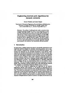
path {a p ε q b} whose cost is at most (1 + 2ε)distP (a, b). Let π ˜ =a b be a shortest path between a and b in P . The path π ˜ consists of segments with end-points on the edges of P . We call these points bending points of the path π ˜ . From our assumption, the 18

a

y(a)

P

b

b y(b)

x(a) a

x(b)

p N (a)

p

Figure 1: A shortest path π˜ = a

P

G

N (b)

q

q

b = {a, x(a), y(a)

mated by an approximate discrete path (dashed) {a

P

N (a)

x(b), y(b), b} between a and b is approxip

Gε

q

N (b)

b}.

path π ˜ intersects more than two faces. There are two subcases to consider - the one where π ˜ remains entirely inside N (a) ∪ N(b) - and the other where the path π ˜ is not entirely in N (a) ∪ N (b). Here we discuss the latter case, and the other one will trivially follow from its proof. We denote by y(a) the first bending point on π ˜ when traversed from a to b, where the path exits N (a) (see Figure 1). Similarly, let x(b) be the last bending point on π ˜ when traversed from a to b, where the path enters N (b). Furthermore, we denote by x(a) the bending point on π ˜ preceding y(a) and by y(b) the bending point succeeding x(b). Let us consider, first, the case where none of the points x(a), y(a), x(b), and y(b) is inside vertex vicinity. By their choice x(a) and y(a) lie on two different sides of the face f containing the segment (x(a), y(a)). We define p to be a Steiner point in f such that |x(a)p| + |py(a)| ≤ (1 + ε/2)|x(a)y(a)|.

(12)

The existence of such a Steiner point is shown in Lemma 2. Similarly, let q be a Steiner point inside the face containing (x(b), y(b)) and such that |x(b)q| + |qy(b)| ≤ (1 + ε/2)|x(b)y(b)|.

(13)

If x(a) = x(b) and y(a) = y(b) we choose p = q. Now we have defined an approximate N (a)

Gε

N (b)

q b} and estimate its cost. discrete path π(a, b) = {a p We consider the case where (x(a), y(a)) 6= (x(b), y(b)) (Figure 1). From the definition of the points x(a) and y(b), and the triangle inequality we have ka and kq

N (a)

N (b)

pk ≤ ka

P

bk ≤ ky(b)

x(a)k + kx(a)pk

(14)

P

(15)

bk + kqy(b)k.

Again from the triangle inequality and the validity of (10) for the path p c(p

Gε

q) ≤ (1 + ε)(ky(a)

P

x(b)k + kpy(a)k + kx(b)qk). 19

Gε

q we obtain (16)

Then the cost of the path π(a, b) is estimated by summing (14), (16), and (15) and using (12), and (13)

ka

N (a)

c(π(a, b)) = ka P

pk + c(p

Gε

P

q) + kq

N (b) P

bk ≤

x(a)k + (1 + ε)ky(a) x(b)k + ky(b) bk + (1 + ε/2)kx(a)y(a)k + (1 + ε/2)kx(b)y(b)k + ε(kpy(a)k + kx(b)qk) ≤ (1 + 2ε)distP (a, b)

The case where segments (x(a), y(a)) = (x(b), y(b)) is simpler. The cases where some of the points x(a), y(a), x(b), and y(b) are inside vertex vicinities are handled by the same technique. Next, we estimate distGε (a, b) from below. Again, we assume that distGε (a, b) < distP (a, b). Otherwise, statement (a) of the theorem holds. We consider any approximate N (a)

N (b)

G

discrete path of the form {a p εq b}. If p is a vertex vicinity node we denote by p˜ the vertex in that vicinity. Correspondingly, r(˜ p) is the weighted radius of p˜ defined by (6). If p is a Steiner point node then p˜ denotes the corresponding Steiner point and we assume r(˜ p) = 0. We use analogous notation q˜ and r(˜ q) for q. From our definitions and using this notation, we have ka

N (a)

pk ≥ ka

P

p˜k − εw(a)r(˜ p) and kq

Then, for the cost of the path {a ka

N (a)

pk + c(p

Gε

q) + kq

N (b)

N (a)

p

bk ≥ ka

Gε

P

q

N (b)

N (b)

bk ≥ k˜ q

P

bk − εw(b)r(˜ q).

(17)

b}, which is distGε (a, b), we obtain

p˜k + c(p

Gε

q) + k˜ q

P

bk − ε(w(a)r(˜ p) + w(b)r(˜ q )). (18)

In the case where w(a)r(˜ p) + w(b)r(˜ q) ≤ ka

P

p˜k + c(p

Gε

q) + k˜ q

P

bk,

we use (18) and (11) and obtain ka

N (a)

(1 − ε)(ka

(1 − ε)2 (ka

(1 − ε)(ka

P

P

pk + c(p

Gε

p˜k + c(p

Gε

P

q) + kq

N (b)

q) + k˜ q

p˜k + (1 − ε)distP (˜ p, q˜) + k˜ q

p˜k + distP (˜ p, q˜) + k˜ q

P

P P

bk ≥

bk) ≥

bk) ≥

bk) ≥ (1 − 2ε)distP (a, b),

(19)

which implies the lower bound in (a). Consider now the case where w(a)r(˜ p) + w(b)r(˜ q) > ka

P

20

p˜k + c(p

Gε

q) + k˜ q

P

bk.

(20)

We show that in this case (b) holds. This inequality is possible only if one of the points p˜ or q˜ is a vertex of P , denoted by v, and the other is either a Steiner point inside the face neighbourhood of v or the same vertex. Furthermore, (20) implies that the points a and b P and any shortest path a b stay in N (v). In the case where p˜ = q˜ = v we use (18) and obtain distGε (a, b) ≥ ka

P

vk + kv

P

bk − ε(w(a) + w(b))r(v) ≥ distP (a, b) − ε(w(a) + w(b))r(v),

which proves the lower bound in (b). If p˜ = v and q˜ is a Steiner point in N (v), then from (17) we have distGε (a, b) ≥ ka

P

vk+c(p

Gε

q)+k˜ q

N (b)

bk−εw(a)r(v) ≥ ka

P

vk+kb

P

vk−ε(w(a)+w(b))r(v),

and the lower bound in (b) holds again. The cases where just one of the points a or b is Steiner point or incident to a vertex vicinity are treated analogously. 2 Next, we make some remarks on the quality of the approximation given by the approximate distances in the cases (a) and (b) of Theorem 4. If case (a) of the theorem applies then the approximate distance distGε (a, b) is an approximation of the distance distP (a, b) |distGε (a,b)−distP (a,b)| , which is bounded by 2ε. Case (b) of the theowith relative error of distP (a,b) rem can be viewed as an exception covering a special situation where points a and b are “close” to each other and “near” a vertex v of P , meaning that any shortest path in P between them stays in the face neighbourhood N (v). Furthermore, in case (b) the approximate distance distGε (a, b) is less than the actual distance distP (a, b) and it is an approximation with relative error not exceeding ε(w(a) + w(b))r(v)/distGε (a, b). Therefore, if (w(a) + w(b))r(v) ≤ 2distGε (a, b) the quality of the approximation is 2ε, same as in case (a). If the ratio r(v)(w(a) + w(b))/distGε (a, b) is larger than 1/ε then the relative error could be as big as 1. For example, if points a and b are inside the vertex vicinity E(v) then distGε (a, b) is zero and the relative error is 1. Note, that the conditions for the occurrence of case (b) and the presence of eventually large (compared to ε) relative error are easily detected by the position of the points a and b, the structure of the approximate discrete path and the ratio (w(a) + w(b))r(v)/distGε (a, b). Thus, if the approximation is not satisfactory the exact shortest path restricted to lie inside N (v) can be computed. Straightforwardly, such computation can be done in time quadratic to the number of faces incident to v, which is efficient if the degree of v is small. Alternatively, additional preprocessing can be done for vertices with large degrees so that exact shortest paths in their face neighbourhoods can be answered efficiently. The above discussion is summarized in the next corollary. Corollary 1 The distance distGε (a, b) approximates distP (a, b) with relative error 2ε, except possibly when the case (b) of Theorem 4 applies and (w(a) + w(b))r(v) > 2distGε (a, b). We conclude this section by a remark on the computation of approximate distances. The approximate distance distGε (a, b) between a pair of points a and b can be computed as follows. 21

We consider the approximate discrete paths of the form (7) and compute the minimum min(ka

N (a)

pk + c(p

Gε

q) + kq

N (b)

bk),

(21)

over all pairs of nodes p ∈ N (a) and q ∈ N (b). In the case where a and b do not lie in neighbour faces this minimum is the approximate distance distGε (a, b). In the case where the points a and b lie in neighbouring faces, we also need to consider the shortest local path between them.

4

Fixed source shortest path queries

In this section, we describe an algorithm, that takes as input a point a in P , called source, and an approximation parameter ε ∈ (0, 1) and constructs a data structure, called Single Source Queries (SSQ), such that for any query point b, called target, the approximate distance distGε (a, b) (and/or an approximate shortest path) from a to b is computed efficiently. (It is assumed that the query consists of the query point b and a pointer to the face of P containing b.) The algorithm uses the approximation graph Gε defined and analyzed in the previous section as follows. First, we construct the set of nodes of the approximation graph Gε , as described in Section 3. Then we augment Gε so that a becomes a representation of a new node in Gε . That is, we add a new node in Gε whose representation in P is a and connect it to all nodes of Gε , whose representations are incident to the face neighbourhood N (a) of the face containing a. A cost equal to the cost of the shortest local path between a and the representation of the corresponding node in N (a) is assigned to each of the new edges. This augmentation of the approximation graph is denoted by Gaε or simply Gε , when no ambiguity arises. The augmentation takes time proportional to the number of the new edges, which by Lemma 3 is O( √1ε log 1ε ). The result of Theorem 4 is extended straightforwardly to the graph Gaε and to the approximate distances distGaε (a, b), where b is an arbitrary point in P . Next, we run the SSSP algorithm on Gaε with source a and store the SSSP tree and the distances as required. Then, for a query point b, we will find the shortest approximate discrete path from a to b and output its cost distGaε (a, b) as an approximation to the distance distP (a, b) and the natural embedding of the path, if required. Approximate discrete paths between the node a and a point b are either local shortest Ga

N (b)

paths, or paths of the form {a ε p b}, where p is a node of Gaε incident to the face neighbourhood of b. Hence, the computation of the approximate distance distGaε (a, b) requires finding min (distGaε (a, p) + kp

p∈N (b)

N (b)

bk)

(22)

and the cost of the shortest local path between a and b if they lie in neighbouring faces. The cost of the shortest local path when necessary is computed in constant time. So we concentrate on the computation of (22).

22

We have already computed and stored the distances distGaε (a, p) from a to all nodes p ∈ Gaε and thus our task is reduced to finding a node p(b) that minimizes (22) for a query point b. Next, we introduce the notion of Local Voronoi Diagrams between a pair of adjacent faces and show how that can be used in finding the node p(b) as required in (22). More precisely, let f be a face of P and let N (f ) be its face neighbourhood consisting of at most three faces. Each of these faces in turn have Steiner points which have been placed on their corresponding bisectors. The distance of the path from a to b that we are interested in passes through one of these Steiner points. Our objective is to locate that Steiner point that satisfies Equation (22). For each face f ′ ∈ N(f ) we compute the Steiner point that satisfies this equation and then take the minimum among all the neighbouring faces. We will compute an additively weighted Voronoi Diagram of the set of Steiner points in f ′ , with respect to the distance distGaε , and restrict this diagram to f . We call the resulting diagram as the Local Voronoi Diagram and denote it by LVD(a, f ′ , f ). Given this diagram, for a query point b ∈ f , we will be able to efficiently compute the Voronoi region which contains b, and hence the Steiner point in face f ′ that satisfies the equation (22). Next, we state how we carry out the construction of LVD(a, f ′, f ) and perform point location in it. Let f = ABC and, without loss of generality, let e = AB be horizontal, where f is above AB, and A is to the left of B. Let f ′ be the face adjacent to e. Without loss of generality let p1 , p2 , . . . , pk be the set of Steiner points in f ′ ordered according to their increasing distance from a. First, we will compute LVD of these points on e, denoted by LVD(a, f ′ , e), and then propagate it to the interior of the face f . The Voronoi diagram on e is computed in an incremental fashion, by considering Steiner points in increasing order of their distances to a. Assume that we have already computed LVD(a, f ′ , e) with respect to Steiner points p1 , . . . , pi (where, i < k) and now we wish to update this diagram to include the effect of the next Steiner point pi+1 . Due to the convexity and the continuity of the distance measure, Voronoi cell of pi+1 on e, with respect to Voronoi cells of p1 , . . . , pi will either be empty or will consist of a single interval; denote this interval by [x− , x+ ]. Let M be an endpoint of one of the intervals characterizing the Voronoi diagram of p1 , . . . , pi . The relative position of M with respect to the interval [x− , x+ ] on e can be computed in constant time. Hence, using binary search we can find the location of the endpoints x− and x+ on e and update the diagram within this interval. Since each newly inserted element occupies at most one interval, it is easy to see that there are, in all, at most 2k − 1 intervals on e. They can be maintained in a search tree structure by naturally following their containment order. Next, we propagate the Voronoi diagram to the interior of the face f . Note that LVD(a, f ′ , f ) has the following combinatorial structure: Voronoi cells are connected, each cell has a non-empty intersection with e, and it has at most 2k − 1 cells. We use plane sweep, in the +y direction starting at e. In place of computing the full diagram, we compute the diagram for a set of horizontal segments in f , parallel to e, that correspond to ‘events’. These events represent combinatorial changes in LVD, which in turn corresponds to the end of a Voronoi cell for a Steiner point. The events are maintained in a priority queue with respect to their increasing distance from e. Initially the events are derived from adjacent intervals on

23

e; each interval endpoint is the intersection point of e and the bisector (i.e., locus of all points that are equidistant) between two Steiner points. During the sweep, intervals disappear one by one and the adjacency between the intervals changes, which gives rise to new events. For horizontal lines corresponding to two consecutive event points, there are only O(1) changes in the LVDs, and the corresponding interval structure can be maintained using the persistent tree structure of [39]. It can be seen that LVD for horizontal lines corresponding to events in f can be encoded in O(k log k) time. Given a query point b ∈ f , we locate the Voronoi region of LVD(a, f ′, f ) containing b as follows. First we perform a binary search with respect to its distance from e to locate the two adjacent horizontal lines corresponding to event points in which b lies. Let these lines be e′ and e′′ , where e′ is further than e′′ with respect to distance from e. Using the persistent tree structure we know the interval structure on e′ and e′′ , and we also know the set of Steiner points in f ′ that contribute these intervals. Note that the interval structure is same between e′ and e′′ , except that one of the intervals has disappeared on e′′ . Consider an interval endpoint in e′′ and its corresponding endpoint in e′ . Furthermore, we know the equation of the curve (bisector) that joins these two endpoints. In constant time we can test whether b is to the left or to the right of this curve (for example this can be accomplished by intersecting this curve with the horizontal line passing through b). Therefore, using binary search we can locate the Voronoi cell containing b in O(log k) time. As stated above, our objective was to locate that Steiner point that satisfies Equation (22). To do this for each face f ′ ∈ N(f ), using the LVD(a, f ′ , f ), we compute the Steiner point that satisfies this equation and then take the minimum among all the neighbouring faces. In the next lemma we summarize the above discussion. Lemma 4 Let p1 , . . . , pk be the set of Steiner points and the vertices of P incident to N (f ) and let δi = distGε (a, pi ) for i = 1, . . . , k. A data structure exists so that for a point b ∈ f the N (b)

minimum min1≤i≤k (δi + kpi bk) and the point for which it is achieved can be computed in O(log k) time. The size of the data structure is O(k) and it can be constructed in O(k log k) time.

We define SSQ(a; P, ε), data structure to consists of the SSSP tree rooted at a in the approximation graph Gaε plus the collection of local Voronoi diagrams LVD(a, f ′ , f ) for all pairs of neighbouring faces f, f ′ ∈ P . This data structure can be used to answer single source queries as follows. We assume that each query consists of the query point b on P as well as the face f (b) containing b. First, using the LVD data structure we find the point p(b) for which the minimum (22) is achieved. Then, if a and b lie in neighbour faces, we compute the shortest local path between a and b and output the approximate distance distGaε (a, b), which is the smaller of the two values. If an approximation path is required we output the natural embedding of the approximate discrete path whose cost is distGaε (a, b). The quality of this approximation follows from Theorem 4 and Corollary 1. The above discussion is summarized in the next theorem.

24

Theorem 5 Given a triangulated, weighted surface P with n faces, a point a ∈ P and the set of nodes Vε of Gε , a data structure SSQ(a; P, ε) of size O(|Vε|) = O( √nε log 1ε ) exists, so that the approximate distance between a and a query point b in P can be found in O(log 1ε ) time. The data structure can be constructed in O(|Vε| log |Vε |) = O( √nε log nε log 1ε ) time. Proof: Follows from the above discussion and using Lemma 3, Lemma 4, and Theorem 3. 2

5

Arbitrary shortest path queries

In this section, we describe and analyze an algorithm for constructing a data structure, called All Pairs Queries (APQ), such that approximate distance (and/or approximate shortest paths) queries between pairs of arbitrary points in P can be answered efficiently. In addition to the weighted polyhedral surface P and the approximation parameter ε, the algorithm takes as input a query time parameter q and outputs a data structure APQ(P, ε; q), which can answer approximate distance queries in O(q) time (the parameter q is within a range of values and it is made precise in the theorem at the end of this section). Our approach is based on the results obtained in the previous two sections. First, we compute the set of Steiner points and vertex vicinities defining the set of nodes Vε of the approximation graph Gε . Then, we consider the dual graph P ∗ of P , defined as follows. The set of nodes of P ∗ corresponds to the set of faces of P and two nodes in P ∗ are joined by an edge if their corresponding faces are neighbours. To each node u of P ∗ we assign the weight w(u) equal to the number of nodes of Gε , that are incident to the face f (u) in P . Furthermore, we assign the cost c(u) equal to the number of nodes of Gε , that are incident to the face neighbourhood N (f (u)). The total weight w(P ∗) of P ∗ and the value σ(P ∗ ), defined in Section 2, are estimated using Lemma 3 by n 2 2 n w(P ∗) ≤ C(P ) √ log and σ(P ∗ ) ≤ Γ(P ) log2 , (23) ε ε ε ε P P 2 ∗ where C(P ) = n1 f ∈P C(f ) and Γ(P ) ≤ 16 f ∈P C (f ). We observe that the weight of P n ∗ and σ(P ) are related by σ(P ∗ ) ≤ 16w 2(P ∗ ) ≤ 16nσ(P ∗ ). (24)

Next, we choose a value t ∈ (0, 1) depending on the input query time q and use Theorem 2 to construct a t-separator S, that induces a regular partitioning of P ∗ . The separator S of P ∗ corresponds to a set of faces in P , which we refer to as face separator (or simply separator) and denote again by S. The face separator S partitions the surface P into regions, that are unions of faces corresponding to the connected components of P ∗ \ S. The boundary ∂R of a region R is the set of triangles in S, that neighbour faces in R. Finally, we use Theorem 5 and construct a collection of SSQ data structures depending on the region partitioning defined by the face separator S. The collection of SSQ data structures and the region partitioning induced by S constitutes the APQ(P, ε; q) data structure. We refer to the construction of the APQ data structure as preprocessing and present it in more 25

detail in Table 4. We denote the genus of the surface P by g. The query time parameter q 2/3 1/3 will not exceed an upper bound ¯q defined by ¯q = (g+1)√ε n . APQ Preprocessing Input: A weighted polyhedral surface P of genus g and consisting of n triangular faces; an approximation parameter ε ∈ (0, 1); 2/3 1/3 query time parameter q ≤ ¯q = (g+1)√ε n . Output: Data structure APQ(P, ε; q). Step 1. Define the set of nodes of Gε by computing the Steiner points and vertex vicinities of P . Step 2. Construct the dual graph P ∗ and assign weights and costs to its nodes as specified above. Step 3. Set t =

q2 4(g+1)σ(P ∗ ) log2

1 ε

Using Theorem 2, compute a t-separator S and construct the region partitioning of P induced by S. Step 4. For each p, that is a Steiner point or vertex of P incident to a face, which neighbours a face in S compute and store SSQ(p; P, ε) data structure. Step 5. For each region R and for each Steiner point or vertex of P incident to a face in R compute and store SSQ(p; R, ε) data structure restricted to the faces in R. Table 4: All Pairs Queries Preprocessing algorithm In the next lemma we estimate the time for the construction and the size of APQ(P, ε; q) data structure. Lemma 5 For any q ≤ ¯q =

(g+1)2/3 n1/3 √ ε

by the preprocessing algorithm takes

the construction of the data structure APQ(P, ε; q)

2 O( (g+1)n ε3/2 q

log nε log4 1ε ) time. The size of APQ(P, ε; q) is

2

O( (g+1)n log4 1ε ). ε3/2 q Proof: We estimate the time following the steps as presented in Table 4. By Lemma 3, Step 1 takes O( √nε log 1ε ) time. The time for the execution of Step 2 is O(n). According to Theorem 2, Step 3 is executed in O(n log n) time. Recall that t = q2 /(4(g +1)σ(P ∗) log2 1ε ). To estimate the times for the execution of Steps p 4 and 5 we use Theorems 5 and 2. In Step 4, we compute O( (g + 1)σ(P ∗)/t) SSQ data structures in O(w(P ∗) log w(P ∗)) time each. The sizes of these data structures are bounded by O(w(P ∗)). In Step 5 for each region R defined by the separator S we construct SSQ data structures restricted to R. The number of these structures in R equals the total weight of the faces in 26

R, which we denote by w(R). By Theorem 3, the construction of each of these SSQ data structures is O(w(R) log w(R)) and their size is bounded by O(w(R)). Overall, the time for the execution of Step 5 is bounded by O(tw 2(P ∗ ) log w(P ∗ )). The total size of the SSQ data structures stored in Step 5 is O(tw 2(P ∗ )). Finally, we use w 2 (P ∗ ) ≤ nσ(P ∗ ) and observe that under the assumption q ≤ ¯q the time used by Step 4 dominates the execution time used by Step 5, and consequently, the total time of the whole preprocessing algorithm. Similarly, the total size of the SSQ data structures stored during Step 4 is bigger than the total size of the structures stored during Step 5. Thus, the asymptotic bounds on the time required by the algorithm and the size of the output are obtained by evaluation of the time and size used by Step 4 in terms of n and ε. We use the estimates (23). 2 The APQ data structure built by the preprocessing algorithm can be used to answer approximate distance queries in the following way. Let a and b be points in P and let f (a) and f (b) be the faces containing a and b respectively. We use APQ(P, ε; q) to compute the approximate distance distGε (a, b), defined as the cost of the shortest approximate discrete path between a and b. By definition, approximate discrete paths are either local shortest paths or paths of the N (a)

Gε

N (b)

q b}. In the case where f (a) and f (b) are neighbours we form (7), which is {a p compute the shortest local path between a and b. Then, we concentrate on finding the cost of a shortest path of the form (7), i.e. computing the minimum (21). Recall, that APQ(P, ε; q) contains a collection of SSQ data structures as specified in Steps 4 and 5 in the preprocessing algorithm. If a data structure SSQ(p′ ; P, ε) is present in APQ(P, ε; q) for some node p′ of Gε , then we can use it and find the minimum cost of an approximate discrete path between a and b among the paths containing p′ . We simply compute distGε (a, p′ ) and distGε (p′ , b), using SSQ(p′ ; P, ε) twice, and sum them up. By Theorem 5, this computation takes O(log 1ε ). Thereby we introduce the notion of separating set of nodes of Gε for a pair of points a and b. A set of nodes Gε is called separating set for a and b if any approximate discrete path of the form (7) between a and b contains a node from that set. Our query algorithm specifies a separating set A for a and b, such that for any p′ ∈ A the data structure SSQ(p′ ; P, ε) is present in APQ(P, ε; q) and then computes the minimum minp′∈A (distGε (a, p′ )+distGε (p′ , b)). Clearly, this minimum is the cost of the shortest approximate discrete path of the form (7). The time for this computation is O(|A| log 1ε ). In Table 5, we present the query algorithm. If an approximate shortest path between a and b is required we output the natural embedding of the approximate discrete path for which the minimum distGε (a, b) is achieved. This can be done by using the SSSP trees stored in the corresponding SSQ data structure in time proportional to the size of this path. The next lemma establishes the correctness of the query algorithm and evaluates its running time. Lemma 6 The algorithm APQ Query correctly computes the approximate distance distGε (a, b). The running time of the algorithm is O(max(q, √1ε log2 1ε )). Proof: The correctness of the query algorithm follows from the observation, that the cost of any approximate discrete path between a and b is given by the values M0 , M1 and M2 , 27

APQ Query Input: Query points a and b and faces f (a) and f (b), such that a ∈ f (a) and b ∈ f (b). Output: The approximate distance distGε (a, b). Set M0 = M1 = M2 = ∞.

Step 1. If f (a) and f (b) are neighbour faces, then compute the shortest local path a

f (a)∪f (b)

b and assign its cost to M0 .

Step 2. If either of the faces f (a) or f (b) is in the separator S, then define A to be the set of nodes of Gε incident to the face neighbourhood N (a) or N (b), respectively.

Step 3. If neither of the faces f (a) and f (b) is in S, then define A to be the set of nodes of Gε incident to the faces in the boundary ∂R(a) of the region R(a) containing f (a). Step 4. Use data structures SSQ(p′ ; P, ε) and compute M1 = minp′∈A (distGε (a, p′ ) + distGε (p′ , b)).

Step 5. If f (b) ∈ R(a) then define A1 to be the set of nodes of Gε incident to the face neighbourhood N (b). Use data structures SSQ(p′ ; R(a), ε) and compute M2 = minp′ ∈A1 (distGε (a, p′ ) + distGε (p′ , b)). Set distGε (a, b) = min(M0 , M1 , M2 ) and output it. Table 5: The APQ Query algorithm answers approximate shortest path queries between arbitrary points on P in O(q) time using APQ(P, ε; q). depending on the position of the faces f (a) and f (b) with respect to the partitioning defined by the separator S. The running time of the algorithm is dominated by the times for the execution of Steps 4 and 5. As discussed above these times are bounded by O(|A| log 1ε ) and O(|A1| log 1ε ). By Lemma 3, |A1 | = O( √1ε log 1ε ) and by Theorem 2 and the choice of t in the p APQ Preprocessing algorithm we obtain |A| ≤ 2 (g + 1)tσ(P ∗) ≤ logq 1 . 2 ε The results obtained in this section are summarized in the next theorem. Theorem 6 Let P be a weighted polyhedral surface of genus g and consisting of n trian2/3 1/3 gular faces. Let ε ∈ (0, 1) and q ∈ ( √1ε log2 1ε , ¯q = (g+1)√ε n ). There exists a data structure APQ(P, ε; q), such that approximate distance queries in P can be answered in O(q) 2 log nε log4 1ε ) time and its size is time. The structure APQ(P, ε; q) is constructed in O( (g+1)n ε3/2 q 2

O( (g+1)n log4 1ε ). ε3/2 q

28

6

Improved APQ data structure for surfaces of genus zero

In this section, we consider a surface P of genus zero4 (i.e. P is homeomorphic to a planar domain). We refer to this as P being planar. We show that when P is planar it is possible to construct, a data structure which is improved in terms of its size, for answering distance queries between arbitrary pairs of points on P . We refer to this data structure as planar APQ data structure and denote it by PAPQ(P, ε; q). Roughly speaking the size of the planar APQ data structure is reduced by a factor of qε3/2 , whereas the preprocessing time is increased 1 by a factor of ε− 2 compared to the general APQ data structure described in the previous section. More precisely we are going to show that the following theorem holds: Theorem 7 Let P be a weighted polyhedral surface of genus zero consisting of n tri1/4 angular faces. Let ε ∈ (0, 1) and q ∈ ( 1ε log2 1ε , n ε ). There exists a data structure APQ(P, ε; q), such that approximate distance queries in P can be answered in O(q) time. 2 The structure PAPQ(P, ε; q) is constructed in O( εn2 q log q log nε log4 1ε ) time and its size is 2

O( εn3 q2 log2 q log6 1ε ). The key in the construction and analysis of the planar APQ data structure, as stated in Theorem 7, is the observation that shortest paths in the approximation graph Gε inherit some planar properties from the surface P . These properties allow us to answer queries efficiently while using less stored information. First we describe the PAPQ data structure and present a preprocessing algorithm, called as PAPQ Preprocessing, for its construction. Next, we analyze the preprocessing algorithm and establish upper bounds on the size of the data structure and time required for its construction in terms of the input parameters. Then we describe, analyze and prove the correctness of a query algorithm. The algorithms are obtained following the approach used in the general case; hence in our presentation we emphasize the differences. As in the general case, the preprocessing algorithm takes as input an approximation 1/4 parameter ε ∈ (0, 1) and a query parameter q not exceeding ¯q′ = n ε and produces a data structure that is later used for answering shortest path queries in P . The algorithm is presented formally in Table 6. The first three steps of the PAPQ Preprocessing algorithm are the same as in the APQ Preprocessing algorithm, except for a slightly different separation parameter t′ in Step 3. At the end of Step 3, we obtain a partitioning of the faces of P into sets called regions and a special single set S called separator. Each region corresponds to a connected subgraph of P ∗ and no two faces from different regions are neighbours. The number of nodes of Gε incident to the faces in any region R is bounded by t′ w(P ∗), i.e. w(R) ≤ t′ w(P ∗). The boundary of a region R is defined as the set of faces in S that neighbour faces in R and is denoted by ∂R. In Step 3, the preprocessing algorithm computes and stores the boundary ∂R of each region following the order in which the triangles forming that boundary appear around R. This order is well defined in the planar case, since the edges shared by any of our regions and its boundary form a cycle. 4

The genus of P can be easily computed using Euler’s formula.

29

of the regions is bounded by p pAccording to Theorem 2 the cost of the boundaries ′ ∗ ∗ 2 t σ(P ) and the cost c(S) of the separator is O( σ(P )/t′ ), where σ(P ∗ ) is the sum of the squares of the costs of the faces in P . Our PAPQ Preprocessing algorithm consists of three more steps. In these, we compute a collection of shortest path distances and a collection of so called partial SSQ data structures that will form the PAPQ(P, ε; q) data structure. A partial SSQ data structure SSQ(p; F, ε) from p to a set of faces F ⊂ P is defined as the set of Local Voronoi Diagrams LVD(p, f ′ , f ) from p to all faces f ∈ F , where f ′ ∈ N(f ). Note that the partial SSQ data structure does not store the shortest paths from p to the nodes of Gε incident to faces neighbouring faces in F . It stores diagrams LVD(p, f ′ , f ) for f ∈ F only. From Lemma 4 it follows, straightforwardly, that the partial SSQ data structures, SSQ(p; F, ε), have size O(w(F )) and can be constructed in O(w(F ) log w(F )) time, provided that the distances from p to the nodes in the faces neighbouring F are computed in advance. We denote by N (S) the set of faces that neighbour faces in S, i.e N (S) = ∪f ∈S N (f ). In Step 4, the algorithm computes distances and partial SSQ data structures related to nodes in Gε , that are incident to faces in N (S). That is, for each node p ∈ N (S) the following three sub-steps are implemented. First (in Step 4.1) the SSSP tree in Gε rooted at p is computed. The distances distGε (p, q) from p to all nodes q ∈ N (S) are stored in the PAPQ(P, ε; q) data structure. Then, in Step 4.2 the algorithm computes and stores partial SSQ data structures SSQ(p; S, ε) from nodes p ∈ N (S) to faces in S. Step 4.3 is implemented for nodes that are incident to faces in S only. For any such node p up to three more partial SSQ data structures with source p are computed and stored. That is, for each of the regions R(p) neighbouring the face containing p (recall that p is incident to a face in S) the partial SSQ data structure SSQ(p; R(p), ε) is computed and stored. Note that, although SSSP trees rooted at nodes in N (S) were computed, they are not stored in the planar APQ data structure. Instead carefully selected collection (related to the separator S) of partial SSQ data structures have been computed and stored. As a result the size of the obtained APQ data structure is considerably reduced compared to the one in the general case. To describe Step 5, we introduce the notion of restricted distances with respect to a region in Gε . A node p of Gε is said to be inside a region R if p is incident to faces in R only. Nodes that are not inside R are said to be outside of R. Definition 2 For a region R and a pair of nodes p and q outside R we define the restricted distance between p and q with respect to R to be the least cost of a path in Gε between p and q that avoids nodes inside R. We denote the restricted distance between p and q with respect to R by c(p

Gε \R

q).

Clearly, the restricted distances from a node p outside of R to all other nodes q outside R with respect to R can be computed by running the SSSP algorithm from p in the subgraph of Gε obtained by removal of all nodes inside R. The upper bound on the running time of the SSSP algorithm as stated in Theorem 3 applies in this case too. In Step 5, the PAPQ Preprocessing algorithm considers all pairs (p, R(p)), where p is a node incident to a 30

face f (p) ∈ S and R(p) is a region neighbouring f (p) (or equivalently f (p) ∈ ∂R(p)), and computes the restricted distances with respect to R(p) from p to all nodes q outside of R(p). The restricted distances from p to nodes q, that are incident to faces in S, are stored in the PAPQ(P, ε; q) data structure. Step 6 of the PAPQ Preprocessing algorithm is same as Step 5 of the preprocessing algorithm in the general case (see Table 4). Recall, that in this step the algorithm computes and stores the SSQ data structures SSQ(p; R, ε) for all regions R computed in Step 3 and nodes p incident to faces in R. PAPQ Preprocessing Input: A weighted polyhedral surface P of genus zero and consisting of n triangular faces; an approximation parameter ε ∈ (0, 1); 1/4 query time parameter q ≤ ¯q′ = n ε . Output: Data structure PAPQ(P, ε; q). Implement Steps 1 and 2 of APQ Preprocessing algorithm (Table 4). Step 3. Set t′ =

q2 ε 4σ(P ∗ ) log2 q log2

1 ε

. Using Theorem 2, compute a t′ -separator S.

Construct the region partitioning of P induced by S. Compute and store the boundary of each region in sorted order. Step 4. For each node p ∈ Gε that is incident to a face in N (S) implement Steps 4.1 – 4.3 below: Step 4.1. Compute SSSP tree in Gε rooted at p. Step 4.2. Compute and store partial SSQ data structures SSQ(p; S, ε). Step 4.3. If p ∈ S then for any region R(p) neighbouring the face incident to p compute and store SSQ(p; R(p), ε). Step 5. For each node p incident to a face f ∈ S and for each region R neighbouring f compute and store restricted distances c(p from p to all nodes q, incident to faces in S.

Gε \R

q)

Step 6. For each region R and for each node p incident to a face in R compute and store SSQ(p; R, ε) data structure. Table 6: Planar All Pairs Queries Preprocessing algorithm The next lemma establishes upper bounds on the running time of PAPQ Preprocessing algorithm and on the size of the PAPQ(P, ε; q) data structure. Lemma 7 For q ≤

n1/4 ε

2

the

the PAPQ Preprocessing algorithm takes O( εn2 q log q log nε log4 1ε ) 2

time. The size of the PAPQ(P, ε; q) data structure is O( εn3 q2 log2 q log6 1ε ).

31

Proof: First we estimate the running time of the preprocessing algorithm. As we have shown in the proof of Lemma 5, the total time for the execution of the first three steps is bounded by O( √nε log nε ). The data stored in the PAPQ data structure during the first three steps is O( √nε log 1ε ). According to Theorem 2, the number of the SSSP trees computed in Step 4.1 p σ(P ∗ ) log qlog 1ε √ is O( σ(P ∗ )/t′ ), that is O( ). By Theorem 3, each of these computa(q ε) ∗ ∗ tions takes O(w(P ) log w(P )) and hence the time for the execution of Step 4.1 is σ(P ∗ )w(P ∗ ) log w(P ∗ ) log q log 1ε √ ). O( (q ε) As stated above, the time for computation of a partial SSQ data structure SSQ(p; F, ε) is proportional to w(F ) log w(F ), where, by our definitions, w(F ) is the number of nodes incident to faces in F . The size of this data structure is O(w(F )). Thereafter, the running time of Step 4.2 is O(w(N (S))w(S) log w(S)). By our definitions this is O(c(S)w(S) log w(S)), σ(P ∗ )w(S) log w(S) log q log 1ε √ ). Clearly, this bound is asympwhich, using the bound on c(S), is O( (q ε) totically less than the bound obtained for Step 4.1. The size of the SSQ data structures stored during Step 4.2 is O(w(N (S))w(S)), which is bounded by c2 (S). The latter by Theorem 2 σ2 (P ∗ ) log2 qlog2 1ε ). is O(σ(P ∗)/t′ ), which after substitution of t′ is O( εq2 ′ ∗ ′ ∗ Step 4.3 runs in O(w(S)t w(P ) log(t w(P ))), which as shown below, is dominated by the running time of Step 6. Similarly, the size of the SSQ data structures stored during this step is asymptotically less than the size of the SSQ data structures stored by Step 6. Restricted distances in Step 5 are computed using SSSP algorithm, and hence, the time for its execution satisfies the same asymptotic upper bound as Step 4.1. The number of the restricted distances stored in Step 5 is bounded by c2 (S), which coincides with the bound obtained for the data stored during Step 4.2. Step 6 is same as Step 5 in APQ Preprocessing algorithm for the general case and its running time was estimated in the proof of Lemma 5 to be O(t′ w 2 (P ∗) log w(P ∗)). The size of the SSQ data structures stored during this step is O(t′w 2 (P ∗ )). By substitution of t′ and using (24), we obtain, that both, the running time and the size of the data stored in Step 6 1/4 is O(εq2n). For q ≤ ¯q′ = n ε , this is asymptotically less than the running time of Step 4.1 and also asymptotically less than the size of the data structures stored in Step 4.2. σ(P ∗ )w(P ∗ ) log w(P ∗ ) log qlog 1ε √ ). The Overall, the running time of the PAPQ Algorithm is O( q ε σ2 (P ∗ ) log2 q log2

1

ε size of the PAPQ(P, ε; q) data structure is O( ). The estimates stated in the εq2 lemma are obtained from these using (23). 2 Next, we describe our query algorithm, called PAPQ Query. The algorithm resembles the structure of the APQ Query algorithm as presented in Table 5, but differs in the way some of the steps are implemented. Thereby, in our presentation below we follow and refer to Table 5. The PAPQ Query algorithm takes as input query points a and b together with the faces f (a) and f (b), containing a and b, respectively. The output of the algorithm is the approximate distance distGε (a, b) between a and b in P (see Definition 1). As in the general case, the distance distGε (a, b) is found as the minimum of three values M0 , M1 , and M2 corresponding to the cost of the shortest path among particular types of

32

discrete paths between a and b. Initially M0 , M1 , and M2 are set to infinity. The value M0 corresponds to the cost of the shortest local path between a and b, i.e., if a and b lie in the neighbouring faces f (a) and f (b), respectively, then the shortest path between a and b lying inside the union f (a) ∪ f (b) is computed and its cost is assigned to M0 . The value M1 corresponds to the cost of the shortest approximate discrete path of the form (7), i.e. M1 =

min

p∈N (a),q∈N (b)

(ka

N (a)

pk + c(p

Gε

q) + kq

N (b)

bk).

The query algorithm uses the PAPQ data structure and properly selected separating sets, depending on the positions of a and b with respect to the separator S, to compute M1 efficiently. Recall, that a set A of nodes in Gε is called separating set for a and b if any approximate discrete path between a and b contains a node in A. In the case where both faces f (a) and f (b) are in S, the algorithm sets the separating set A to be the set of nodes incident to N (b) and computes the minimum M1 using the N (b)

bk). Observe, that the SSQ data structures formula M1 = minq∈A (distGε (a, q) + kq SSQ(q; S, ε) from nodes q ∈ A to the faces in S are present in the PAPQ data structure and so the distances dGε (a, q) are computed in O(log 1ε ) time. The shortest local path and N (b)

correspondingly the distance kq bk is computed in constant time. We have |A| = 1 1 O( √ε log ε ) and thus M1 is computed in O( √1ε log2 1ε ) time. The case where just one of the faces f (a) and f (b) is in S is treated similarly. Without loss of generality, assume that f (a) is in S and f (b) is not. Then f (b) must be in one of the regions defined by S. We denote this region by R(b). In this case, the algorithm uses separating set A consisting of all nodes in Gε that are incident √ to faces in the boundary q ε ∂R(b) of R(b). By Theorem 2 the size of A does not exceed log σ(P ∗ ) log 1 . Then, the algorithm ε

computes M1 using the formula M1 = minq∈A (distGε (a, q) + distGε (q, b)). For any node q in A both SSQ data structures SSQ(q; S, ε) and SSQ(q; R(b), ε) are stored in the PAPQ data structure and therefore M1 can be computed in O(|A| log 1ε ) time, which is at most O(q). The case where the faces f (a) and f (b) belong to different regions, say R(a) and R(b) respectively, is central to our presentation. Planarity of P is essentially used by our query algorithm in this case. To find the minimum M1 in this case, we use a pair of separating sets A(a) and A(b) consisting of the nodes in Gε that are incident to the faces in ∂R(a) and ∂R(b), respectively. Then the algorithm finds the minimum M1 by computing min

p∈A(a),q∈A(b)

(distGε (a, p) + c(p

Gε \R(a)

Gε \R(a)

q) + distGε (q, b)),

(25)

where c(p q) is the restricted distance between p and q with respect to the region R(a). By our definitions it is easily seen that this minimum equals to M1 . Next, we describe how our query algorithm computes (25). First, we observe that for any pair of nodes p ∈ A(a) and q ∈ A(b) the SSQ data Gε q) are present structures SSQ(p; R(a), ε) and SSQ(q; R(b), ε), as well as the distance c(p in the PAPQ(P, ε; q) data structure. Thus, the three terms in (25) for any fixed pair of 33

nodes p and q can be computed in O(log 1ε ) time. The number of such pairs, however, can be large and searching over all pairs to compute (25) is unacceptable. Therefore, we use a more elaborate approach and devise a recursive procedure, called search min (a, b), to compute M1 . The procedure uses the circular structure of the boundaries ∂R(a) and ∂R(b) and properties of shortest approximate discrete paths related to the planarity of P . First we introduce some notation. For a given face f ∈ ∂R(a), let M1 (f ) be the minimum defined by M1 (f ) =

min

p∈A(f ),q∈A(b)

(distGε (a, p) + c(p

Gε \R(a)

q) + distGε (q, b)),

(26)

where, A(f ) is the subset of A(a) consisting of the nodes of Gε incident to f . We consider pairs of nodes (p, q) for which this minimum is achieved and denote by (p∗ , q ∗ ) the one with Gε \R(a)

smallest restricted distance c(p∗ q ∗ ). The pair (p∗ , q ∗ ) is called optimal pair of nodes for f . The face f ∗ containing q ∗ is called optimal face for f . The corresponding restricted path, with respect to R(a), π ∗ (f ) = π(p∗ , q ∗ ) is called optimal path for f . Observe, that by this definition an optimal path π(p∗ , q ∗ ) does not contain nodes which are inside R(a) or R(b). (It does not contain nodes inside R(a), since it is a restricted shortest path with respect to R(a). It does not contain nodes inside R(b) since q ∗ has been chosen to minimize the Gε \R(a)

restricted distance c(p q) among pairs (p, q) for which the minimum (26) is achieved.) The next lemma establishes an important property of optimal paths. Let f1 and f2 be different faces in ∂R(a) and let π ∗ (f1 ) and π ∗ (f2 ) be optimal paths for f1 and f2 , respectively. Let f1∗ and f2∗ be the optimal faces for f1 and f2 determined by π ∗ (f1 ) and π ∗ (f2 ), respectively. Furthermore, let π ˜ ∗ (f1 ) and π ˜ ∗ (f2 ) be the natural embedding of the paths π ∗ (f1 ) and π ∗ (f2 ) in P . Roughly speaking, the natural embedding of a discrete path is obtained by embedding its edges into their corresponding local shortest paths (see Section 3.2 for more detail). Lemma 8 If the natural embeddings π ˜ ∗ (f1 ) and π ˜ ∗ (f2 ) intersect then the face f1∗ is optimal ∗ for f2 and f2 is optimal for f1 . Proof: Let z be the first point of intersection between π ˜ ∗ (f1 ) and π ˜ ∗ (f2 ) (following the paths starting at f1 and f2 , respectively). Let (p∗1 , q1∗ ) and (p∗2 , q2∗ ) be the optimal pair for f1 and G G G f2 , respectively, for which the minimum (26) is achieved. Let π1 (a, b) = (a ε p∗1 ε q1∗ ε b) denote the shortest path from a to b passing through the optimal pair (p∗1 , q1∗ ). Similarly, let π2 (a, b) denote the shortest path from a to b passing through (p∗2 , q2∗ ). Let π1 (i, j) (or π2 (i, j)) denote the subpath of π1 (a, b) (respectively, π2 (a, b)) between (nodes) i and j. Case 1: Consider the case when z corresponds to a node in Gε . In that case the subpaths π1 (z, b) and π2 (z, b) have equal cost. Construct a new path π12 (a, b) = {π1 (a, z), π2 (z, b)}. We have kπ1 (a, b)k = kπ12 (a, b)k, thus π12 (a, b) is a shortest path intersecting f1 and f2∗ via an optimal pair (p∗1 , q2∗ ). Hence, the face f2∗ is optimal for f1 . (So does f1∗ for f2 .) Case 2: Consider the case when z does not correspond to a node in Gε . It belongs to the intersection of the embedding of two edges e1 = (w1 , v1 ) and e2 = (w2 , v2 ) from π ∗ (f1 ) and π ∗ (f2 ), respectively. We say that point z is isolated if there exists a disk of non-zero radius 34

centred at z that does not contain any other point that is common to π ∗ (f1 ) and π ∗ (f2 ). We consider the case when z is an isolated point in Case 2.a and 2.b, and otherwise in Case 2.c. Case 2a: Let z be an isolated point in the interior of a face, denoted by f (z). Then z is the intersection of two segments corresponding to embeddings of edges e1 and e2 . Let the embedding e˜1 of e1 is represented by two segments e˜1 = {w1 x1 , x1 v1 }, where w1 and v1 correspond to nodes in Gε and x1 is a bending point. Likewise, let the embedding e˜2 of e2 be e˜2 = {w2 x2 , x2 v2 }, where w2 and v2 correspond to nodes in Gε and x2 is a bending point. Without loss of generality assume that z is intersection of x1 v1 and x2 v2 (see Figure 2 (a)). Note that the points (or the corresponding nodes in Gε ) w1 , v1 , w2 , v2 are incident to the face neighbourhood N (z) of z. Thus, by definition, (w1 , v2 ) and (w2 , v1 ) are edges of Gε . Also, the cost of the edge (w1 , v2 ) corresponds to the cost of shortest path connecting the endpoints which is restricted to lie within the face neighbourhood N (z). Same argument holds for the cost of edge (w2 , v1 ). By triangle inequality and the cost of edges, we have N (z)

w1 v2 ≤ w1 x1 + x1 v2 and w2 follows that kw1

N (z)

v2 k + kw2

N (z)

N (z)

v1 ≤ w2 x2 + x2 v1 . Since x1 v2 + x2 v1 < x1 v1 + x2 v2 , it

v1 k < kw1 x1 k + kw2 x2 k + kx1 v1 k + kx2 v2 k = ke1 k + ke2 k

(27)

In case x1 and x2 are also nodes in Gε , then w1 coincides with x1 , w2 coincides with x2 , and (27) is still valid. We construct two paths denoted by π12 (a, b) and π21 (a, b), from a to b, passing through f1 and f2 , respectively, as follows: π12 (a, b) = {π1 (a, w1 ), (w1 , v2 ), π2 (v2 , b)} and π21 (a, b) = {π2 (a, w2 ), (w2 , v1 ), π2 (v1 , b)}. Applying (27), we have kπ12 (a, b)k + kπ21 (a, b)k < kπ1 (a, b)k + kπ2 (a, b)k. Hence, this case contradicts the optimality of the paths that we started with. Case 2b: Let z be an isolated point on an edge of P . Then z must be a bending point as shown in Figure 2(b) and (c). Note that w1 , w2 , v1 , v2 are nodes in Gε and the edges e1 and e2 are denoted by e1 = (w1 , v1 ) and e2 = (w2 , v2 ), respectively. In all possible cases, we have N (z)

N (z)

N (z)

N (z)

kw1 v2 k + kw2 v1 k < kw1 v1 k + kw2 v2 k = ke1 k + ke2 k, which follows the same argument as above. This proves that z can not be an isolated point on an edge of P . Case 2c: Consider now the case where z is not isolated. (The only possibility for z in this case is shown in Figure 2(d).) The embedding of e1 is represented by three segments {w1 x1 , x1 y1 , y1 v1 }, where w1 , v1 are nodes of Gε and they are the endpoints of e1 . Similarly, the embedding of e2 is represented by {w2 x2 , x2 y2 , y2 v2 }. Then x1 , x2 , y1 , y2 are bending points and z is their first common point. Without loss of generality let x2 coincide with z. We have already shown that (w1 , v2 ) and (w2 , v1 ) are edges of Gε . By observation, we have N (z)

N (z)

N (z)

N (z)

kw1 v2 k+kw2 v1 k = kw1 v1 k+kw2 v2 k. As in Case 2a, we define two paths: π12 (a, b) = {π1 (a, w1 ), (w1 , v2 ), π2 (v2 , b)} and π21 (a, b) = {π2 (a, w2 ), (w2 , v1 ), π2 (v1 , b)}. Thus, we have kπ12 (a, b)k+kπ21 (a, b)k = kπ1 (a, b)k+kπ2(a, b)k. Hence, kπ12 (a, b)k = kπ1 (a, b)k and kπ21 (a, b)k = kπ2 (a, b)k must hold. Otherwise, without loss of generality let kπ12 (a, b)k = kπ1 (a, b)k + δ and kπ21 (a, b)k = kπ2 (a, b)k − δ, where δ > 0. This contradicts the optimality of the optimal paths π ∗ (f1 ) and π ∗ (f2 ). Hence, we proved the claim. 2 Recall, that the edges in the region R, that are incident to faces in its boundary ∂R form a cycle. Furthermore, in Step 3 of the preprocessing algorithm the faces in each boundary 35

x2

y1 z

x2

z

x1

y2

x1

y1 y2

(a)

(b)

y1 x2

z x1

y2 u1

v1 v2

u2

x1 x2(z) (c)

y1 y2 (d)

Figure 2: An illustration of the case when point z whose representation is not a node in Gε . (a) Point z is an isolated point in the interior of a face (Case 2.a). (b) and (c) Point z is an isolated point on an edge of P (Case 2.b). (d) Point z is not isolated (Case 2.c).

36

have been stored in the PAPQ data structure sorted according to their appearance around R. So, any pair of different faces f1 and f2 in the boundary ∂R defines a clockwise chain C(f1 , f2 ; ∂R) (or simply C(f1 , f2 ) if no ambiguity arises) consisting of all faces, including f1 and f2 , between f1 and f2 ordered in clockwise direction starting at f1 . We also use the ¯ f ) for the chain consisting notation C(f, f ) for a chain consisting of a single face f and C(f, of all faces in ∂R ordered in clockwise direction starting at f . The size of a chain C(f1 , f2 ) is the number of faces in it and is denoted by |C(f1 , f2 )|. We define median of a chain C(f1 , f2 ) as a face f ∈ C(f1 , f2 ) such that the difference between the sizes of the chains C(f1 , f ) and C(f, f2 ) is at most one. Let f1∗ and f2∗ be the optimal faces for f1 and f2 , respectively, where f1 , f2 are on the boundary of R(a) and f1∗ , f2∗ are on the boundary of R(b). Then, for a chain C = C(f1 , f2 ) on the boundary of R(a), the chain C ∗ = C(f2∗ , f1∗ ) on the boundary of R(b) is said to be the optimal chain (see Figure 3). Furthermore, optimal chains and faces satisfy the following useful relation. π ∗(f1)

f1 R(a)

π ∗(f ) a

C = C(f1, f2)

f∗

z f1∗

f f2

R(b) b

∗

π (f2)

f2∗

C ∗ = C(f2∗, f1∗)

Figure 3: Illustration of an optimal chain Lemma 9 Let C be a chain on ∂R(a) and let C ∗ be a chain on ∂R(b) be optimal chain for C. Then, any face f ∈ C has an optimal face in C ∗ . Proof: Follows from the planarity of P and Lemma 8. See Figure 3. 2 Next we describe our procedure search min(a, b), that computes the minimum (25). The procedure first computes approximate distances distGε (a, p) and dGε (q, b) for all nodes p and q incident to faces in ∂R(a) and ∂R(b), respectively. Then, the procedure picks an arbitrary face f0 on ∂R(a) and computes the minimum M1 (f0 ) and an optimal face f0∗ ∈ ∂R(b) for f0 . ¯ 0 , f0 ), C(f ¯ ∗ , f ∗ )) At the end, search min(a, b) calls a recursive procedure search min(C(f 0 0 and outputs M1 as the smaller of M1 (f0 ) and the value returned by that procedure. Below, we describe the recursive procedure search min(C, C ∗ ). The procedure search min(C, C ∗ ) takes as input a chain C = C(f1 , f2 ) in the boundary of R(a) and an optimal chain C ∗ = C(f2∗ , f1∗ ) for C and computes the minimum M1 (C, C ∗) defined by (25), but over the subsets A(C) ⊂ A(a) and A(C ∗ ) ⊂ A(b), where A(C) consists of all nodes in Gεε incident to faces in C. The set A(C ∗ ) is defined analogously with respect to b. The procedure search min(C, C ∗ ) checks whether any of the chains C and C ∗ consists 37

of a single face and if so computes M1 (C, C ∗ ) by checking all pairs of nodes p ∈ A(C) and q ∈ A(C ∗ ). If both chains contain more than one face then the procedure finds the median face f of C and computes the minimum M1 (f ) =

min

(distGε (a, p) + c(p

p∈A(f ),q∈A(C ∗ )

Gε \R(a)

q) + distGε (q, b)),

(28)

and an optimal face f ∗ for f . Then, the procedure search min(C, C ∗ ) calls recursively search min(C(f1 , f ), C(f ∗, f1∗ )) and search min(C(f, f2 ), C(f2∗ , f ∗ )) and outputs M1 (C, C ∗) = min(M1 (C(f1 , f ), C(f ∗, f1∗ )), M1 (C(f, f2 ), C(f2∗, f ∗ ))).

(29)

The latter is valid because of Lemma 9. Lemma 10 The procedure search min(a, b) correctly computes the minimum (25) in O(max( 1ε log2 1ε , q)) time. Proof: The fact that search min(C, C ∗ ) computes M1 (C, C ∗) follows by induction on the ¯ 0 , f0 ) = ∂R(a) and size of C and using the validity of (29). Then, by definition, we have C(f ∗ ∗ ¯ C(f0 , f0 ) = ∂R(b) and the correctness of search min(a, b) follows. We first estimate the running time of search min(C, C ∗ ). From its description it is easy to see, that the running time of search min(C, C ∗ ) is bounded by T (C ∗ ) log |C|, where T (C ∗ ) is an upper bound on the time for computing the minimum M1 (f ) by (28) for any face f in C. By Lemma 3, the size of the set A(f ) for any face f is O( √1ε log 1ε ) and hence ∗

)| √ T (C ∗ ) = O( |A(C log 1ε ). We have obtained that the running time of search min(C, C ∗ ) is ε )| √ O( |A(C log |C| log 1ε ). On the other hand, if one of the chains consists of a single face, the ε running time of search min(C, C ∗ ) is Ω( 1ε log2 1ε ). The running time of search min(a, b) is the sum of the times for the initialization and ¯ 0 , f0 ), C(f ¯ 0∗ , f0∗ )). The latter is the time taken by the recursive procedure search min(C(f √ O( w(∂R(b)) log |∂R(a)| log 1ε ), where w(∂R(b)) is the number of nodes of Gε incident to faces ε in ∂R(b). By Theorem 2 and the value of the separation parameter t′ we have w(∂R(b)) ≤ √ q ε . From the same estimate on w(∂R(a)) we have that |∂R(a)| ≤ q. Therefore, log q log 1ε ¯ 0 , f0 ), C(f ¯ ∗ , f ∗ )) runs in O(max( 1 log2 1 , q)) time. procedure search min(C(f 0 0 ε ε Partial SSQ data structures SSQ(p; R(a), ε) and SSQ(q; R(b), ε) are present in the PAPQ data structure for all nodes p incident to faces in ∂R(a), and for nodes q incident to faces in ∂R(b). Therefore, each of the distances distGε (a, p) and distGε (q, b) is computed in O(log 1ε ) time. The number of these distances is bounded by the sum w(∂R(a)) + w(∂R(b)), which as √ q ε discussed above is less than 2 log q log 1 . Hence, this computation takes less than O(q) time. ∗

ε

Computing M1 (f0 ) and an optimal face f0∗ ∈ ∂R(b) takes O(max( 1ε log2 1ε , logq q )) time. The lemma follows. 2 Finally, we consider the case where faces f (a) and f (b) belong to a single region R = R(a) = R(b). To find the distance distGε (a, b) in this case, we partition approximate discrete paths 38

between a and b into two groups. The first group consists of approximate discrete paths that stay within R and the second group consists of those that contain nodes outside R. Then, the distance distGε (a, b) is equal to the smaller of the two distances found with respect to the paths in each group. To find the distance with respect to the paths inside R, we define A to be the set of nodes N (a)

in Gε incident to the faces in N (f (a)) and compute minp∈A (ka pk + distR (p, b)). For any p ∈ A the distance distR (p, b) is computed using the SSQ data structure SSQ(p; R, ε) in O(log 1ε ) time. The shortest local path is computed in constant time and therefore the minimum and the distance inside R is computed in O( √1ε log2 1ε ). The distance with respect to paths that leave R is computed in O(q) time. This concludes the description of the PAPQ Query algorithm. We summarize the above discussion in the following lemma. Lemma 11 The algorithm PAPQ Query correctly computes the approximate distance distGε (a, b) in O(max( 1ε log2 1ε , q)) time. The validity of Theorem 7 stated in the beginning of the section follows from Lemmas 7 and 11.

7

Extensions and Conclusions

In this paper, we present novel solutions to fundamental shortest path query problems. The algorithms improve and generalize previous solutions in terms of 1) setting: a) Euclidean to weighted and b) arbitrary genus g, 2) preprocessing time, and/or 3) size of query data structure. We also develop a new graph partitioning algorithm for graphs of genus g with weights and costs on vertices which extends and/or generalizes previously known separator algorithms. Our techniques also enable us to obtain improved results with space-query time tradeoffs for the planar case, i.e., when the genus is 0. A natural question arises whether the range ( √1ε log2 1ε , ¯q) of query time parameter q, in Theorem 6, can be widened, while keeping the efficiency of the algorithm. This question can be answered affirmatively by constructing a hierarchical APQ data structure, in which second level APQ data structures are built and stored for each region of the partitioning. For each region R of the partitioning construct an APQ(R, ε; ¯qR) restricted to R, where ¯qR is the corresponding upper bound for R. Then, in the APQ-Query algorithm we use APQ(R, ε; ¯qR ) to answer approximate shortest path queries in the case where both query points lie in R in O(¯qR) in time. The latter is O(q) since ¯q ≤ q. Our analysis shows that if 5/9 2/3 q ≤ ¯q1 = (g+1)ε2/3 n log7/3 1ε the result of Theorem 6 extends to the case q ∈ (¯q, ¯q1 ). By the same approach the interval for q in the planar case can be extended from above. Next, we briefly describe how our technique can be used to build an APQ data structure with query time parameter q = log 1ε . We build an ε-mesh consisting of O( ε12 ) additional points in each triangle f of P . The mesh is constructed so that for each point a in f there is a mesh point p which is closer to a than εd(p), where d(p) is the minimum distance from 39

2

p to any node of Gε outside f . Then for each mesh point we compute, in O( εn5/2 log nε log 1ε ) time, the SSQ data structure. For a pair of query points a, b we first find the mesh point p(a) closest to a, and then use the structure SSQ(p(a); P, ε) to find distGε (p(a), b). Each of these two steps is carried out in O(log 1ε ) time. It can be shown that kap(a)k + distGε (p(a), b) is an ε-approximation of the distance distP (a, b).

References [1] P. K. Agarwal, B. Aronov, J. O’Rourke, and C. A. Schevon. Star unfolding of a polytope with applications. SIAM J. Comput., 26(6):1689–1713, 1997. [2] P. K. Agarwal, S. Har-Peled, and M. Karia. Computing approximate shortest paths on convex polytopes. Algorithmica, 33(2):227–242, 2002. [3] P. K. Agarwal, S. Har-Peled, M. Sharir, and K. Varadarajan. Approximate shortest paths on a convex polytope in three dimensions. Journal of the ACM, 44(4):567–584, 1997. [4] L. Aleksandrov and H. Djidjev. Linear algorithms for partitioning embedded graphs of bounded genus. SIAM J. Disc. Math., 9(1):129–150, 1996. [5] L. Aleksandrov, H. Djidjev, H. Guo, and A. Maheshwari. Partitioning planar graphs with costs and weights. J. Exp. Algorithmics, 11:1.5, 2006. [6] L. Aleksandrov, H. Djidjev, H. Guo, A. Maheshwari, D. Nussbaum, and J.-R. Sack. Approximate shortest path queries on weighted polyhedral surfaces. In In Proc. 31st Int. Symp., Mathematical Foundations of Computer Science, LNCS 4162, pages 98–109. Springer-Verlag, 2006. [7] L. Aleksandrov, M. Lanthier, A. Maheshwari, and J.-R. Sack. An ε-approximation algorithm for weighted shortest path queries on polyhedral surfaces. In Proc. 14th Euro CG Barcelona, pages 19–21, 1998. [8] L. Aleksandrov, M. Lanthier, A. Maheshwari, and J.-R. Sack. An ε-approximation algorithm for weighted shortest paths on polyhedral surfaces. In Proceedings of SWAT, LNCS 1432, pages 11–22, Berlin, Germany, 1998. Springer. [9] L. Aleksandrov, M. Lanthier, A. Maheshwari, and J.-R. Sack. An improved approximation algorithm for computing geometric shortest paths. In In Proc. Foundations of Computation Theory, LNCS 2751, pages 246–257, Berlin, Germany, 2003. Springer. [10] L. Aleksandrov, A. Maheshwari, and J.-R. Sack. Determining approximate shortest paths on weighted polyhedral surfaces. Journal of ACM, 52(1):25–53, 2005.

40

[11] S. Arikati, D. Chen, L. Chew, G. Das, M. Smid, and C. Zaroliagis. Planar spanners and approximate shortest path queries among obstacles in the plane. In In Proc. of the Forth Annual Fourth Annual European Symposium on Algorithms ESA’96, LNCS 1136, pages 514–528, Berlin, Germany, 1996. Springer-Verlag. [12] J. Canny and J. H. Reif. New lower bound techniques for robot motion planning problems. In Proc. 28th. Annu. IEEE Symposium on Foundations of Computer Sciences, pages 49–60, 1987. [13] B. Chazelle, D. Liu, and A. Magen. Sublinear geometric algorithms. SIAM J. Comput., 35:627–646, 2006. [14] D. Chen. On the all-pairs Euclidean short path problem. In Proc. 6th ACM-SIAM Sympos. on Discrete Algorithms (SODA), pages 292–301, 1995. [15] D. Chen, O. Daescu, and K. Klenk. On geometric path query problems. In Proc. 5th WADS, Lecture Notes in Comp. Sci., 1272:248–257, 1997. [16] D. Z. Chen and J. Xu. Shortest path queries in planar graphs. Proc. 32nd Annu. Symp. Theory Comput. (STOC), pages 469–478, 2000. [17] J. Chen and Y. Han. Shortest paths on a polyhedron. In Proceedings of 6th ACM Symposium on Computational Geometry, pages 360–369, 1990. Full version IJCGA 6: 127-144, 1996. [18] J. Chen and Y. Han. Storing shortest paths for a polyhedron. In Proc. 1991 Int. Conf. on Comp. and Information, volume 497 of LNCS, pages 169–180, 1991. [19] Siu-Wing Cheng, Hyeon-Suk Na, Antoine Vigneron, and Yajun Wang. Approximate shortest paths in anisotropic regions. In Nikhil Bansal, Kirk Pruhs, and Clifford Stein, editors, SODA, pages 766–774. SIAM, 2007. [20] Siu-Wing Cheng, Hyeon-Suk Na, Antoine Vigneron, and Yajun Wang. Querying approximate shortest paths in anisotropic regions. In Jeff Erickson, editor, Symposium on Computational Geometry, pages 84–91. ACM, 2007. [21] Y.-J. Chiang and J. Mitchell. Two-point Euclidean shortest path queries in the plane. In Proc. 10th ACM-SIAM Sympos. on Discrete Algorithms (SODA), pages 215–224, 1999. [22] K. Clarkson. Approximation algorithms for shortest path motion planing. Proc. 19th Annu. Symp. Theory Comput. (STOC), pages 56–65, 1987. [23] H. N. Djidjev. Linear algorithms for graph separation problems. In SWAT’88, LNCS, volume 318, pages 216–222. Springer-Verlag, Berlin, Heidelberg, 1988.

41

[24] Hristo Djidjev. Partitioning planar graphs with vertex costs: Algorithms and applications. Algorithmica, 28(1):51–75, 2000. [25] R. M. Dudley. Metric entropy of some classes of sets with differentiable boundaries. J. Approx. Theory, 10(3):227–236, 1974. [26] G. N. Frederickson. Fast algorithms for shortest paths in planar graphs. SIAM J. Comput., 16:1004–1022, 1987. [27] G. N. Frederickson. Planar graph decomposition and all pairs shortest paths. Journal of ACM, 38(1):162–204, 1991. [28] J. R. Gilbert, J. P. Hutchinson, and R. E. Tarjan. A separator theorem for graphs of bounded genus. J. Algorithms, 5:391–407, 1984. [29] L. Guibas and J. Hershberger. Optimal shortest path queries in a simple polygon. J. Comput. Syst. Sci., 39:126–152, 1989. [30] S. Har-Peled. Approximate shortest paths and geodesic diameters on convex polytopes in three dimensions. Discrete & Comp. Geometry, 21:217–231, 1999. [31] S. Har-Peled. Constructing approximate shortest path maps in three dimensions. SIAM J. Comput., 28(4):1182–1197, 1999. [32] J. Hershberger and S. Suri. An optimal algorithm for Euclidean shortest paths in the plane. SIAM J. Comput., 28:2215–2256, 1999. [33] P. Klein, S. Rao, M. Rauch, and S. Subramanian. Faster shortest-path algorithms for planar graphs. J. Comput. Syst. Sci., 55(1):3–23, 1997. [34] R. J. Lipton and R. E. Tarjan. A separator theorem for planar graphs. SIAM J. Appl. Math., 36:177–189, 1979. [35] J. Mitchell, D. Mount, and C. Papadimitriou. The discrete geodesic problem. SIAM J. of Computing, 16:647–668, 1987. [36] J. Mitchell and C. Papadimitriou. The weighted region problem: Fiding shortest paths through a weighted planar subdivision. Journal of the ACM, 38:18–73, 1991. [37] J. H. Reif and Z. Sun. An efficient approximation algorithm for weighted region shortest path problem. In Proceedings of the 4th Workshop on Algorithmic Foundations of Robotics (WAFR2000), pages 191–203, Hanover, New Hampshire, 2000. A. K. Peters Lt. [38] J. H. Reif and Z. Sun. On finding approximate optimal paths in weighted regions. J. Algorithms, 58:1–32, 2006.

42

[39] N. Sarnak and R. E. Tarjan. Planar point location using persistent search trees. Communications of ACM, pages 669–679, 1986. [40] Y. Schreiber and M. Sharir. Optimal-time algorithm for shortest paths on a convex polytope in tree dimensions. In Proceedings of 22nd ACM Symposium on Computational Geometry, pages 30–39, 2006. [41] M. Sharir and A. Schorr. On shortest paths in polyhedral spaces. SIAM J. Computing, 15:193–215, 1986. [42] Xuehou Tan, Tomio Hirata, and Yasuyoshi Inagaki. Spatial point location and its applications. In Tetsuo Asano, Toshihide Ibaraki, Hiroshi Imai, and Takao Nishizeki, editors, SIGAL International Symposium on Algorithms, volume 450 of Lecture Notes in Computer Science, pages 241–250. Springer, 1990.

43