1
A Framework of Sparse Online Learning and Its Applications
arXiv:1507.07146v1 [cs.LG] 25 Jul 2015
Dayong Wang, Pengcheng Wu, Peilin Zhao, and Steven C.H. Hoi, Abstract—The amount of data in our society has been exploding in the era of big data today. In this paper, we address several open challenges of big data stream classification, including high volume, high velocity, high dimensionality, high sparsity, and high class-imbalance. Many existing studies in data mining literature solve data stream classification tasks in a batch learning setting, which suffers from poor efficiency and scalability when dealing with big data. To overcome the limitations, this paper investigates an online learning framework for big data stream classification tasks. Unlike some existing online data stream classification techniques that are often based on first-order online learning, we propose a framework of Sparse Online Classification (SOC) for data stream classification, which includes some state-of-the-art first-order sparse online learning algorithms as special cases and allows us to derive a new effective second-order online learning algorithm for data stream classification. In addition, we also propose a new costsensitive sparse online learning algorithm by extending the framework with application to tackle online anomaly detection tasks where class distribution of data could be very imbalanced. We also analyze the theoretical bounds of the proposed method, and finally conduct an extensive set of experiments, in which encouraging results validate the efficacy of the proposed algorithms in comparison to a family of state-of-the-art techniques on a variety of data stream classification tasks. Index Terms—online learning; sparse learning; classification; cost-sensitive learning.
✦
1
I NTRODUCTION
In the era of big data today, the amount of data in our society has been exploding, which has raised many opportunities and challenges for data analytic research in data mining community. In this work, we aim to address the challenging real-world big data stream classification task, such as web-scale spam email classification. In general, big data stream classification has several characteristics: • high volume: one has to deal with huge amount of existing training data, in million or even billion scale; • high velocity: new data often arrives sequentially and very rapidly, e.g., about 182.9 billion emails are sent/received worldwide every day according to an email statistic report by the Radicati Group [1]; • high dimensionality: there are a large number of features, e.g., for some spam email classification tasks, the length of the vocabulary list can go up from 10, 000 to 50, 000 or even to million scale; • high sparsity: many feature elements are zero, and the faction of active features is often small, e.g., the spam email classification study in [2] showed that • Dayong Wang is with Department of Computer Science and Engineering, Michigan State University, USA 48824. E-mail:
[email protected] • Pengcheng Wu and Steven C.H. Hoi are with School of Information Systems, Singapore Management University, Singapore 178902. E-mail: {pcwu, chhoi}@smu.edu.sg • ∗ Peilin Zhao, the corresponding author, is with Institute for Infocomm Research, A*STAR, Singapore 138632. E-mail:
[email protected]
accuracy saturates with dozens of features out of tens of thousands of features; and • high class-imbalance: some class considerably dominates the others, e.g., for spam email classification tasks, the number of non-spam (ham) emails is often much larger than the number of spam emails. The above characteristics present huge challenges for big data stream classification tasks when using conventional data stream classification techniques that are often restricted to batch learning setting and thus suffer from several critical drawbacks: (i) it requires a large memory capacity for caching arrived examples; (ii) it is expensive to collect and train on the entire data set; (iii) it suffers from expensive re-training cost whenever new training data arrives; and (iv) their assumption that all training data must be available a prior does not hold for real-world data stream applications where data arrives rapidly in a sequential manner. To tackle the above challenges, a promising approach is to explore online learning methodology that performs incremental training over streaming data in a sequential manner. Typically, an online learning algorithm processes one instance at a time and makes very simple updates with each arriving example repeatedly. In contrast to batch learning algorithms, online algorithms are not only more efficient and scalable, but also able to avoid expensive re-training cost when handling new training data, making them more favorite choices for solving large-scale machine learning tasks towards big data stream applications. In literature, a large variety of algorithms have been proposed, including a number of first-order algorithms [3], [4] and second-order algorithms [5], [6], [7]. Despite being studied extensively,
2
traditional online-learning algorithms suffer from critical limitation for high-dimensional data. This is because they assume at least one weight for every feature and most of the learned weights are often nonzero, making them of low efficiency not only in computational time but also in memory cost for both training and test phases. Sparse online learning [8] aims to overcome this limitation by inducing sparsity in the weights learned by an online-learning algorithm. In this paper, we introduce a framework of Sparse Online Learning for solving large-scale high-dimensional data stream classification tasks. We show that the proposed framework covers some existing first-order sparse online classification algorithm, and is able to further derive new algorithms by exploiting the second order information. The proposed sparse online classification scheme is far more efficient and scalable than the traditional batch learning algorithms for data stream classification tasks. We further give theoretical analysis of the proposed algorithm and conduct an extensive set of experiments. The empirical evaluation shows that the proposed algorithm could achieve state-of-the-art performance. The rest of this paper is organized as follows. Section 2 reviews related work. Section 3 presents our problem formulation. Section 4 proposes our novel framework. Section 5 discusses our experimental results, and section 6 concludes this work. As a summary, our main contributions include: • We propose a general online learning framework, which can easily derive first order and second order algorithms. • We provide general theoretical analysis including general regret and mistake bounds for the proposed algorithms. • The proposed algorithms are evaluated on several high-dimensional large-scale benchmark databases, where the state-of-the-art performances are archived.
online learning algorithms include Perceptron [3], [17], Passive-Aggressive (PA) algorithms [4], etc. The most well-known method is the Perceptron algorithm [3], [17], which updates the model by adding a new example as a support vector with some constant weight. Recently, a series of sophisticated online learning algorithms have been proposed by following the criterion of maximum margin learning principle [18], [19], [4]. One famous algorithm is the Passive-Aggressive (PA) algorithm [4], which evolves a classifier by suffering less loss on the current instance without moving far from the previous function. In recent years, the design of many efficient online learning algorithms has been influenced by convex optimization tools. Furthermore, it was observed that most previously proposed efficient online algorithms can be jointly analyzed based on the following elegant model [20]: Algorithm 1 Online Convex Optimization Scheme INPUT : A convex set Rd for t = 1, . . . , T do predict a vector wt ∈ Rd ; receive a convex loss function ℓt : S → R; suffer loss ℓt (wt ); end for Based on the previous framework, we can consider online learning as an algorithmic framework for convex online learning problem: X min f (w) = min ℓt (w), w
w
t
where f (w) is a convex empirical loss function for the sum of losses over a sequence of observations. The regret of the algorithm is defined as follows: RT =
T X t=1
2
R ELATED WORK
Our work is closely related to the studies of online learning in machine learning and data mining. Below we briefly review some important related works. 2.1 Online Learning Online learning represents a family of efficient and scalable machine learning algorithms [9], which would online optimize some performance measure including, accuracy [4], AUC [10], cost-sensitive metrics [11], etc. Unlike batch learning methods that suffer from expensive re-training cost, online learning works sequentially by performing highly efficient (typically constant) updates for each new training data, making it highly scalable for data stream classification. In literature, various techniques [12], [3], [4], [13], [14], [15], [16] have been proposed for online learning. The well-known first-order
ℓt (wt ) − min w
T X
ℓt (w),
t=1
where w is any vector in the convex space Rd . The goal of online learning algorithm is to find a low regret scheme, in which the regret RT grows sub-linearly with the number of iteration T . As a result, when the round number T goes to infinity, the difference between the average loss of the learner and the average lost of the best learner tends to zero. Although the general online learning algorithms (e.g., Perceptron and PA) have solid theoretical guarantees and performs well on many applications, generally they are limited in several aspects. First, the general online learning algorithms exploit the full features, which is not suitable for large-scale high-dimensional problem. To tackle this limitation, the sparse online learning has been extensively studied recently. Second, the general online learning algorithms only exploit the first order information and all features are adopted the same learning rate. This problem can be addressed by second order online
3
learning algorithms. Last but not least, the general online learning algorithms are not suitable for the imbalance input data streams, which can be efficiently solved by the cost-sensitive online learning algorithms. In the following parts, we will briefly introduce several representative algorithms in the previous three aspects. 2.2 Sparse Online Learning Sparse online learning [21], [8] aims to learn a sparse linear classifier, which only contains limited size of active features. It has been actively studied [21], [22], [23], [24]. There are two group of solutions for sparse online learning. The first group study on sparse online learning follows the general idea of subgradient descent with truncation. For example, Duchi and Singer propose the FOBOS algorithm [21], which extends the Forward-Backward Splitting method to solve the sparse online learning problem in two phases: (i) an unconstrained subgradient descent step with respect to the loss function, and (ii) an instantaneous optimization for a trade-off between minimizing regularization term and keeping close to the result obtained in the first phase. The optimization problem in the second phase can be efficiently solved by adopting simple soft-thresholding operations that perform some truncation on the weight vectors. Following the similar scheme, Langford et al. [8] argue that truncation on every iteration is too aggressive as each step modifies the coefficients by only a small amount, and propose the Truncated Gradient (TG) method which truncates coefficients every K steps when they are less than a predefined threshold θ. The second group study on sparse online learning mainly follows the dual averaging method of [25], can explicitly exploit the regularization structure in an online setting. For example, One representative work is Regularized Dual Averaging(RDA) [22], which learns the variables by solving a simple optimization problem that involves the running average of all past subgradients of the lost functions, not just the subgradient in each iteration. Lee et al. [26] further extends the RDA algorithm by using a more aggressive truncation threshold and generates significantly more sparse solutions. 2.3 Second-order Online Learning Second Order Online Learning aims to dynamically incorporate knowledge of observed data in earlier iteration to perform more informative gradient-based learning. Unlike first order algorithms that often adopt the same learning rate for all coordinates, the second order online learning algorithms adopt different distills to the step size employed for each coordinate. A variety of second order online learning algorithms have been proposed recently. Some technique attempts to incorporate knowledge of the geometry of the data observed in earlier iterations to perform more effective online updates. For example, Balakrishnan et al. [27] propose algorithms
for sparse linear classifiers in the massive data setting, which requires O(d2 ) time and O(d2 ) space in the worst case. Another state-of-the-art technique for second order online learning is the family of confidenceweighted (CW) learning algorithms [13], [28], [29], [30], [16], which exploit confidence of weights when making updates in online learning processes. In general, the second order algorithms are more accurate, converge faster, but fall short in two aspects (i) they incur higher computational cost especially when dealing with highdimensional data; and (ii) the weight vectors learned are often not sparse, making them unsuitable for highdimensional data. Recently, Duchi et al. address the sparsity and second order update in the same framework, and proposed the Adaptive Subgradient method [31] (Ada-RDA), which adaptively modifies the proximal function at each iteration to incorporate knowledge about geometry of the data. 2.4 Cost-Sensitive Online Learning Cost-sensitive classification has been extensively studied in data mining and machine learning. In the past decade, a variety of cost-sensitive metrics have been proposed to tackle this problem. For example, the weighted sum of sensitivity and specificity [32], and the weighted misclassification cost [33], [34]. Both cost-sensitive classification and online learning have been studied extensively in data mining and machine learning communities, respectively. There are only a few works on cost-sensitive online learning. For example, Wang et al. [11] proposed a family of cost-sensitive online classification framework, which are designed to directly optimize two well-known costsensitive measures. Zhao and Hoi [35] tackle the same problem by adopting the double updating technique and propose Cost-Sensitive Double Updating Online Learning (CSDUOL).
3 S PARSE O NLINE L EARNING S TREAM C LASSIFICATION
FOR
DATA
In this section, we first introduce a general sparse online learning framework for online data stream classification, and then provide the theoretical analysis on the framework. The framework will be used to derive the family of first-order and second-order sparse online classification algorithms in the following section. 3.1 General Sparse Online Learning Without loss of generality, we consider the sparse online learning algorithm for the binary classification problem, which is also mentioned as sparse online classification problem in this paper. The sparse online classification algorithm generally works in rounds. Specifically, at the round t, the algorithm is presented one instance xt ∈ Rd , then the algorithm predicts its label as yˆt = sign(wt⊤ xt ),
4
where wt ∈ Rd is linear classifier maintained by the algorithm. After the prediction, the algorithm will receive the true label yt ∈ {+1, −1}, and suffer a loss ℓt (wt ). Then, the algorithm would update its prediction function wt based on the newly received (xt , yt ). The standard goal of online learning is to minimize the number of mistakes suffered by the online algorithm. To facilitate the analysis, we firstly introduce several functions. Firstly, the hinge loss ℓt (w; (xt , yt )) = [1 − yt w⊤ xt ]+ , where [a]+ = max(a, 0), is the most popular loss function for binary classification problem. Given a series of δ-strongly convex functions Φt=1,...,T , with respect to the norms k · kΦt and the dual norms k · k∗Φt . The proposed general sparse online classification (SOC) algorithm is shown in Algorithm 2.
where the final inequality is due to Fenchel’s inequality. In addition, we have ∆t = Φ∗t (θt+1 ) − Φ∗t (θt ) + Φ∗t (θt ) − Φ∗t−1 (θt ) η2 ≤ Φ∗t (θt ) − Φ∗t−1 (θt ) − ηt (∇Φ∗t (θt ))⊤ zt + t kzt k2Φ∗t . 2δ Combining the above two inequalities, we get − ≤
t=1
+
=
=
Φ∗T (θT +1 ) − Φ∗0 (θ1 ) = Φ∗T (θT +1 )
≥
w⊤ θT +1 − ΦT (w),
t=1
t=1
[Φ∗t (θt ) − Φ∗t−1 (θt ) +
d X
wt,i zt,i =
d X i=1
ηt2 kzt k2Φ∗t ]. 2δ
(2)
sign(ut,i )[|ut,i | − λt ]+ zt,i
X
[|ut,i | − λt ]+ |zt,i | −
X
|ut,i ||zt,i | +
X
ut,i zt,i +
ut,i zt,i ≥0
≤
(1)
for any w, and any λ > 0. Proof: Firstly, define ∆t = Φ∗t (θt+1 ) − Φ∗t−1 (θt ), then ∆t
T X
i=1
T h i X η2 Φ∗t (θt ) − Φ∗t−1 (θt ) + t kzt k2Φ∗t + ηt λt kzt k1 , 2δ t=1
T X
ηt2 kzt k2Φ∗t ]. 2δ
ηt (ut − w)⊤ zt
wt⊤ zt =
In this section, we analysis the regret RT of the general sparse online learning (SOL) algorithm. Firstly, we will present a key lemma, which will facilitate the following analysis. Lemma 1: Let Φt , t = 1, . . . , T be δ-strongly convex functions with respect to the norms k·kΦt and let k·k∗Φt be the respective dual norms. Let Φ(0) = 0, and x1 , . . . , xT be an arbitrary sequence of vectors in Rd . Assume that algorithm 2 is run on this sequence with the function Φt , Then, we have the following inequality
t=1
∆t
t=1
Now, we would connect wt⊤ xt and u⊤ t xt as follows:
3.2 Theoretical Bound Analysis
ηt (wt − w)⊤ zt ≤ ΦT (w)
t=1
T X
[Φ∗t (θt ) − Φ∗t−1 (θt ) − ηt u⊤ t zt +
≤ ΦT (w) +
≤
T X
t=1 T X
ηt w⊤ zt − ΦT (w) ≤
Rearranging the above inequality, we get T X
Algorithm 2 General Sparse Online Learning (SOL) INPUT :λ, η INITIALIZATION : θ1 = 0. for t = 1, . . . , T do receive xt ∈ Rd ; ut = ∇Φ∗t (θt ); wt = arg minw 12 kut − wk22 + λt kwk1 ; predict yˆt = sign(wt⊤ xt ); receive yt and suffer ℓt (wt ) = [1 − yt wt⊤ xt ]+ ; if ℓt (wt ) > 0 then θt+1 = θt − ηt zt , where zt = ∇ℓt (wt ); end if end for
T X
ut,i zt,i ≥0
ut,i zt,i ≥0
X
X
[|ut,i | − λt ]+ |zt,i |
ut,i zt,i 0 and A0 = I. It is easy to verify that Φt is 1-strongly convex with respect to kwk2Φt = w⊤ At w. Its dual function
PT where the final inequality used t=1 1t ≤ [log(T ) + 1]. Secondly, the second term of the right hand side can be upper bounded as T X
−1 x⊤ t At xt
=r
t=1
T X t=1
≤ −r
T X t=1
log(
(1 −
det(At−1 ) ) det(At )
det(At−1 ) ) = r log(det(AT )). det(At )
6
Combining the above two inequalities gives ⊤
w AT w 2η η (4) + r log(det(AT )) + λX[log(T ) + 1]. 2 PT x x⊤ Since AT = I + t=1 tr t , its eigenvalue µi satisfies RT ≤
T T X X kxt k22 xt x⊤ t ) = 1+ . µi ≤ 1 + trace( r r t=1 t=1
As a result, we have det(AT ) =
d Y
i=1
µi ≤ (1 +
X2 d T) . r
Plugging the above inequality into (4) will concludes this theorem. Remark: According to this theorem, adopt the second order information for the sparse online learning does further minimize the regret bound to an order of O(log(T )). 4.3 Diagonal Algorithm
Algorithm 5 Diagonal Second Order Sparse Online Learning INPUT :λ, η INITIALIZATION : θ1 = 0. for t = 1, . . . , T do receive xt ∈ Rd ; −1 −1 At−1 diag(xt x⊤ t )At−1 A−1 = A−1 ; −1 ⊤ t t−1 − r+x A x t
specif icity =
T− −M− , T−
sum = µ+
Although the previous second order algorithm significantly reduced the regret bound than the first order algorithm, it will consume O(d2 ) time, which limits its application to real-world high dimension problems. To keep the computational time still O(d) similar with the traditional online learning, we further explored its diagonal version, which will only maintain a diagonal matrix. Its details are in the Algorithm (5).
A−1 t θt ;
anomaly detection, where the class distribution is often highly imbalanced. In this section, we propose a costsensitive sparse online classification algorithm by extending the sparse online learning framework for online anomaly detection tasks. Without loss of generality, we assume the positive class is the rare class in a set of streaming data, which contains more positive examples than negative samples. We will prefer a high cost/lost value when a positive sample is misclassified, while a small cost/lost value when a negative sample is misclassified. Specifically, we respectively denote the number of positive samples and negative sample by T+ and T− ; and M+ , M− are the number of false negative and false positive, respectively. We denote T = T+ + T− and M = M+ + M− . Instead of using the cost-insensitive metric accuracy = T −M T , researchers have proposed a variety of cost-sensitive metrics. One well-know cost-sensitive + and metric is the weighted sum of sensitivity = T+T−M +
t−1
t
ut = wt = sign(ut ) ⊙ [|ut | − λt ]+ ; predict yˆt = sign(wt⊤ xt ) and receive yt ∈ {−1, 1}; suffer ℓt (wt ) = [1 − yt wt⊤ xt ]+ ; θt+1 = θt + ηLt yt xt ; end for
In the following experiments, we mainly adopt the diagonal second order sparse online learning algorithm unless otherwise specified, which is also denoted as “SSOL”. 4.4 Cost-Sensitive Algorithm For the previous algorithms, the classifier is costinsensitive, which suffers the same cost/lost when the positive samples and the negative samples are misclassified. It is inappropriate for many data stream classification tasks in real-world applications, such as online
which is defined as follows:
T− − M− T+ − M+ + µ− , T+ T−
where µ+ + µ− = 1 and 0 ≤ µ+ , µ− ≤ 1 are two parameters to trade off between sensitivity and specificity. In general, the higher the sum value, the better the classification performance. Notably, when µ+ = µ− = 0.5, the corresponding sum is the well known balanced accuracy [32]. In general, the higher the sum value, the better the classification performance. To maximize the sum value, based on the previous framework, we propose a costsensitive sparse online classification algorithm following the theoretical analysis in [11], [35]. In particular, we adopt a modified hinge loss function: (ρIyt =1 + Iyt =−1 )[1 − yt w⊤ xt ]+ , + T− where ρ = µµ− T+ and Iv is an indicator function, which Iv = 1 if v is true, otherwise Iv = 0. In our experiment, we use the balance accuracy as the metric and set µ+ = µ− = 0.5. Generally, it is difficult to predict the number of positive and negative samples T+ and T− in advance. So a more realistic setting is to use two weight parameters c+ and c− for the positive and negative losses, respectively. Hence, the loss function is reformulated as:
(c+ Iyt =1 + c− Iyt =−1 )[1 − yt w⊤ xt ]+ . Denoting ct = c+ Iyt =1 + c− Iyt =−1 , the modified regret is derived as follow: X X RT = ct ℓt (wt ) − ct ℓt (w), t
yt wt⊤ xt ]+ .
t
where ℓt (wt ) = [1 − Based on the proposed sparse online learning framework and the cost-sensitive loss function, we can achieve
7
Algorithm 6 Cost-Sensitive First Order Sparse Online Learning (CS-FSOL) INPUT : λ, η, c+1 , c−1 INITIALIZATION : θ1 = 0, A0−1 = I. for t = 1, . . . , T do receive xt ∈ Rd ; wt = sign(θt ) ⊙ [|θt | − λt ]+ ; predict yˆt = sign(wt⊤ xt ) and receive yt ∈ {−1, 1}; suffer ℓt (wt ) = [1 − yt wt⊤ xt ]+ ; θt+1 = θt + ηcyt Lt yt xt ; end for
the cost-sensitive first order sparse online learning algorithm (CS-FSOL) shown in Algorithm 6. For this algorithm, it is easy to observe that if we treat ηcyt as ηt , then it is the special case of the proposed framework (2) with Φt (w) = 21 kwk22 . So, we would like to prove a new corollary for the proposed framework (2), under the situation that ηt = ηcyt . This can be achieved by combining Lemma 1 with ηcyt [ℓt (wt ) − ℓt (w)] ≤ ηt (wt − w)⊤ zt . Specifically, we have the following corollary: Corollary 4: Under the assumptions of Lemma 1, if we further assume ℓ is convex and ηt = ηcyt , then PT PT the regret RT = t=1 cyt ℓt (w) t=1 cyt ℓt (wt ) − minw of the proposed framework (2) satisfies the following inequality RT ≤
T X
η ΦT (w) + [ kcyt zt k2Φ∗t + λt kcyt zt k1 ] + η 2δ t=1
PT
∗ t=1 ∆t
η
, (5)
where ∆∗t = Φ∗t (θt ) − Φ∗t−1 (θt ). Given the above corollary, we can prove the following theorem for Algorithm 6. Theorem 5: Let (x1 , y1 ), . . . , (xT , yT ) be a sequence of examples, where xt ∈ Rd , yt ∈ {−1, +1} and kxt k1 ≤ X for all t. If further set λt = ηλ, then the regret P P RT = Tt=1 cyt ℓt (wt ) − minw Tt=1 cyt ℓt (w) suffered by the algorithm (6) is bounded as follows: RT ≤
1 2 2 kwk2
η
kwk2 , (X 2 +2λX)(T+ c+ +T− c− )
we could
have
RT ≤ D
t
t−1
t
ut = A−1 t θt ; wt = sign(ut ) ⊙ [|ut | − λt ]+ ; predict yˆt = sign(wt⊤ xt ) and receive yt ∈ {−1, 1}; suffer ℓt (wt ) = [1 − yt wt⊤ xt ]+ ; θt+1 = θt + ηcyt Lt yt xt ; end for
It is easy to verify that this algorithm is the special case of the proposed framework (2), when ηt = ηcyt and Φt (w) = 12 w⊤ At w. So, the corollary 4 holds for this algorithm. Using this corollary, we can prove the following theorem for Algorithm 7. Theorem 6: Let (x1 , y1 ), . . . , (xT , yT ) be a sequence of examples, where xt ∈ Rd , yt ∈ {−1, +1} and kxt k1 ≤ X for all t. If further set λt = λ/t, then the regret PT PT RT = t=1 cyt ℓt (wt ) − minw t=1 cyt ℓt (w) suffered by the algorithm (4) is bounded as RT ≤
D2 η X2 + cmax rd log(1 + T ) + cmax λX[log(T ) + 1], 2η 2 r
for any w ∈ {w |w⊤ AT w ≤ D2 }, where cmax = max(c+ , c− ). The proof of this theorem is omitted, since it is easy and can mainly follows the one for Theorem 3.
5
E XPERIMENTS
In this section, we conduct an extensive set of experiments to evaluate the performance of the proposed sparse online classification algorithms on both synthetic and real datasets. 5.1 Experimental Setup
T T X ηX + ηλcyt X, cy t X 2 + 2 t=1 t=1
for any w ∈ Rd . Further setting η = √
Algorithm 7 Cost-Sensitive Second Order Sparse Online Learning (CS-SSOL) INPUT : λ, η, c+1 , c−1 INITIALIZATION : θ1 = 0, A−1 0 = I. for t = 1, . . . , T do receive xt ∈ Rd ; −1 −1 At−1 xt x⊤ −1 t At−1 A−1 t = At−1 − r+x⊤ A−1 x ;
p (X 2 + 2λX)(T+ c+ + T− c− ),
for any w ∈ {w |kwk2 ≤ D}. We omit the proof, since it is easy. In addition, we can also get the cost-sensitive second order sparse online classification (CS-SSOL) algorithm shown in Algorithm 7. However, its time complexity and space complexity are relatively high for high dimension datasets, we will only use its diagonal variant in practice, where only a diagonal A−1 is maintained and updated. t
In our experiments, we compare the proposed algorithms with a set of state-of-the-art algorithms, including the sparse online learning algorithms and the costsensitive online learning algorithms. The methodology details of these algorithms are listed in Table 1. The three existing algorithms (CS-OGD, CPA and PAUM) are costsensitive online learning without sparsity regularizer. To examine the binary classification performance, beside the synthetic dataset, we evaluate all the previous algorithms on a number of benchmark datasets from web machine learning repositories. Table 2 shows the details of all the datasets in our experiments. These datasets are selected to allow us evaluate the algorithms on various characteristics of data, in which the number of training examples ranges from thousands to millions, feature dimensionality ranges from hundreds to about
8
TABLE 1 List of Compared Algorithms. Algorithm
1st/2nd Order
Sparsity
Description
STG FOBOS Ada-FOBOS Ada-RDA FSOL SSOL
First Order First Order Second Order Second Order First Order Second Order
Truncate Gradient Truncate Gradient Truncate Gradient Dual Averaging Dual Averaging Dual Averaging
Stochastic Gradient Descent [8] FOrward Backward Splitting [21] Adaptive regularized FOBOS [31] Adaptive regularized RDA [31] The proposed Algorithm 3 The proposed Algorithm 5
CS-OGD CPA PAUM CS-FSOL CS-SSOL
First Order First Order First Order First Order Second Order
Non-Sparse Non-Sparse Non-Sparse Dual Averaging Dual Averaging
Cost-Sensitive Online Gradient Descent [11] Cost-Sensitive Passive-Aggressive [4] Cost-Sensitive Perceptron Algorithm with Uneven Margin [36] The proposed Algorithm 6 The proposed Algorithm 7
5.2 Experiment on Synthetic Dataset To evaluate if the proposed sparse online learning algorithm is able to identify effective features for learning the models, we design the first experiment on a synthetic dataset, which allows us to control the exact numbers of effective/noisy feature dimensions. In particular, we generate a synthetic dataset with high dimensionality and high sparsity by following the similar scheme in [28], [29], which contains a set of effective feature dimensions that are correlated with the class labels and a set of noisy feature dimensions that are uncorrelated with the labels.
Specifically, we generate the synthetic dataset with 100, 000 training examples and 10, 000 test examples in R1000 . For each example, the first 100 dimensions are drawn from a multivariate Gaussian distribution with diagonal covariance. Each dimension of the mean vector is uniformly sampled from −1 to 1, and each dimension of covariance is uniformly sampled from 0.5 to 100. We generate the split plane the same as the mean vector. To introduce noisy feature dimensions, we randomly choose 200 noise dimensions out of the rest 900 dimensions for each example. Noises are drawn from a Gaussian distribution of N (0, 100). 8
50 STG FOBOS Ada−FOBOS Ada−RDA FSOL SSOL
45 40
test error rate (%)
16-million, and the total number of non-zero features on some dataset is more than one billion. For the very largescale WEBSPAM dataset, we run the algorithms only once. The sparsity as shown in the last column of the table denotes the ratio of non-active feature dimensions, as some feature dimensions are never active in the training process, which is often the case for some realworld high-dimensional dataset, such as WEBSPAM. We conduct experiments by following standard online learning settings for training a classifier, where an online learner receives a single training example at each iteration and updates the model sequentially. We will examine how different sparsity levels affect test error rate of the classifier trained from a single pass through the training data. Besides, we also measure time cost of different algorithms to evaluate the computational efficiency. To make a fair comparison, all the algorithms adopt the same experimental settings. We use hinge loss as the loss function for the applicable algorithms. To identify the best set of parameters, for each algorithm on each dataset, we conduct a 5-fold cross validation for grid searching the parameters with the fixed sparsity regularization parameter λ = 0. In particular, the learning rates are searched from 2−1 to 29 and the other parameters are searched from 2−5 to 25 . With the best tuned parameters, each algorithm is evaluated for 5 times with a random permutation of a train set. All the experiments were conducted on a Linux server (with Intel Xeon CPU E5-2620 @2.00GHz, 4 CPU cores, 8GB memory) and the programming environment is based on C++ implementation compiled by g++.
35
7
6
30
5
25 4
20 15
3
10 2 5 0
0
20
40
60
80
100
1 80
85
90
95
100
sparsity (%)
Fig. 1. Test error rate of sparse online classification on synthetic dataset. We evaluate all the cost-insensitive sparse online classification algorithms on the synthetic dataset. Figure 1 shows the test error rates of all the compared algorithms, where the right diagram is a sub-figure of the left one with sparsity from 80% to 100%. Several observations can be drawn from the experimental results. First of all, we observe that the test error rates of the truncate gradient based algorithms (STG, FOBOS, Ada-FOBOS) decrease significantly when the sparsity level increases. By contrast, for the dual averaging based algorithms (FSOL, Ada-RDA, SSOL), the test error rates keep stable or even decrease when the sparsity level increases; But the test error rate increases dramatically when the sparsity level is higher than 90%—the actual
9
TABLE 2 List of real-world datasets in our experiments. DataSet
Balance
AUT PCMAC NEWS RCV1 URL WEBSPAM URL2 WEBSPAM2
True True True True True True False False
#Train
#Test
#Feature Dimension
#Nonzero Features
Sparsity(%)
40,000 1,000 10,000 781,265 2,000,000 300,000 1,000,000 100,000
22,581 946 9,996 23,149 396,130 50,000 100,000 10,000
20,707 7,510 1,355,191 47,152 3,231,961 16,071,971 3,231,961 16,071,971
1,969,407 55,470 5,513,533 59,155,144 231,249,028 1,118,027,721 114,852,082 224,201,808
3.07 3.99 29.88 8.80 7.44 95.82 44.96 96.19
sparsity level used for generating the synthetic data. The result indicates that the dual averaging based algorithms more effectively exploit the sparsity in the dataset. Similar observation was also reported in [22] who argued that the dual averaging based methods take more aggressive truncations and thus can generate significantly more sparse solutions. Second, the proposed secondorder algorithm SSOL achieves the lowest error rate among all the compared algorithms, especially for high sparsity level. This observation can be seen more clearly in the right diagram of Figure 1. The above encouraging experimental results indicate that the proposed SSOL algorithm can effectively exploit the sparsity for solving the sparse online classification tasks.
T+ \ T− 1 \ 0.33 1 \ 1.00 1 \ 1.50 1 \ 1.11 1 \ 2.02 1 \ 0.64 1 \ 99 1 \ 99
indicates that the dual averaging technique and second order updating rules are effective to boost the classification performance. Finally, when the sparsity is high, an essential requirement for high-dimensional data stream classification tasks, the proposed SSOL algorithm consistently outperforms the other algorithms over all the evaluated datasets. For example, when the sparsity is about 99.8% for the WEBSPAM dataset (the total feature dimensionality is 16, 609, 143), the test error rate of SSOL is about 0.3%, while the Ada-RDA is 0.4% and the Ada-FOBOS is 0.55%, as shown in Figure 2 (f).
5.4 Running Time on Large Real Datasets 5.3 Test Error Rate on Large Real Datasets In this experiment, we compare the proposed algorithms (FSOL and SSOL) with the other cost-insensitive algorithms on several real-world datasets. Table 2 shows the details of six datasets, which can be roughly grouped into two major categories: the first two datasets (AUT and PCMAC) are general binary small-scale datasets and the corresponding experimental results are shown in Figure 2 (a)-(b); and the rest four datasets (NEWS, RCV1, URL, and WEBSPAM) are large-scale high-dimensional sparse datasets and the corresponding experimental results are shown in Figure 2 (c)-(f). We can draw several observation from these results as follows. First of all, we observe that most algorithms can learn an effective sparse classification model with only marginal or even no loss of accuracy. For example, in Figure 2 (d), the performances of all the algorithms are almost stable when sparsity level is smaller than 80%. It indicates that all the compared sparse online classification algorithm can effectively explore the low level sparsity information. Second, for most cases, we observe that there exists some sparsity threshold for each algorithm, below which test error rate does not change much; but when sparsity level is greater than the threshold, test error rate gets worse quickly. Third, we observe that the dual averaging based second order algorithms (Ada-RDA and SSOL) consistently outperform the other algorithms (STG, FOBOS, FSOL, and Ada-FOBOS), especially for high sparsity level. This
We also examine time costs of different sparse online classification algorithms, and the experiment results are shown in Figure 3. In this experiment, we only adopt the four high-dimensional large-scale dataset. Several observations can be drawn from the results. First of all, we observe that when the sparsity level is low, the time costs are generally stable; on the other hand, when the sparsity level is high, the time cost of the second other algorithms sometimes will somewhat increase. For example, the test costs of Ada-FOBOS, AdaRDA and FSOL in Figure 3 (b) & (d). One possible reason may be that when the sparsity level is high, the model might not be informative enough for prediction and thus may suffer significant more updates. Since secondorder algorithms are more complicated than first-order algorithms, they are more sensitive to the increasing number of updates. Second, we can see that the proposed SSOL algorithm runs more efficiently than another second-order based algorithms (Ada-RDA and Ada-FOBOS). It is even sometimes better than the first order based algorithm (e.g. FOBOS and STD). However, the first order FSOL algorithm is consistently faster than the second order SSOL algorithm. In summary, from the above analysis, we found that the proposed SSOL algorithm is able to achieve the comparable or even better accuracy of existing secondorder algorithms, but has the comparably small time cost as state-of-the-art first-order algorithms with truncated gradient methods.
10
50
10
5
40
70 STG FOBOS Ada−FOBOS Ada−RDA FSOL SSOL
60
test error rate (%)
15
60 STG FOBOS Ada−FOBOS Ada−RDA FSOL SSOL
test error rate (%)
test error rate (%)
20
30 20
50
STG FOBOS Ada−FOBOS Ada−RDA FSOL SSOL
40
30
10 20 75
80
85
90
95
0 70
100
75
80
sparsity (%)
6
5 4.5
7 6.5 6 5.5 5
95
96
97
98
99
4 93
100
5
4
85
90
95
94
95
96
6.4
19
98
99
18 99
100
99.2
99.4
6.2 6 5.8 5.6
1.8
100
4 3.5
2
2
99.8
(c) NEWS
3 2.5
STG FOBOS Ada−FOBOS Ada−RDA FSOL SSOL
2 1.5 1 0.5
96
97
98
99
0 97
100
97.5
98
98.5
99
99.5
100
sparsity (%)
2.2 STG FOBOS Ada−FOBOS Ada−RDA FSOL SSOL
99.6
sparsity (%)
sparsity (%)
test error rate (%)
test error rate (%)
6.6
97
STG FOBOS Ada−FOBOS Ada−RDA FSOL SSOL
sparsity (%)
7
100
18.5
3
0 95
100
99.5
20
1
80
99
19.5
test error rate (%)
test error rate (%)
test error rate (%)
10
6.8
21 20.5
6 5
98.5
STG FOBOS Ada−FOBOS Ada−RDA FSOL SSOL
(b) PCMAC
STG FOBOS Ada−FOBOS Ada−RDA FSOL SSOL
75
98
sparsity (%)
25
0 70
21.5
4.5 94
97.5
22
(a) AUT
15
97
sparsity (%)
STG FOBOS Ada−FOBOS Ada−RDA FSOL SSOL
sparsity (%)
20
100
test error rate (%)
7.5
5.5
4 93
95
8 STG FOBOS Ada−FOBOS Ada−RDA FSOL SSOL
test error rate (%)
test error rate (%)
7 6.5
90
sparsity (%)
8 7.5
85
1 STG FOBOS Ada−FOBOS Ada−RDA FSOL SSOL
0.8
test error rate (%)
0 70
1.6 1.4
0.6
STG FOBOS Ada−FOBOS Ada−RDA FSOL SSOL
0.4
0.2
1.2
5.4 90
92
94
96
sparsity (%)
(d) RCV1
98
100
1 98
98.5
99
sparsity (%)
(e) URL
99.5
100
0 99
99.2
99.4
99.6
99.8
100
sparsity (%)
(f) WEBSPAM
Fig. 2. Test error rate on 6 large real datasets. (a)-(b) are two general datasets, (c)-(f) are four large-scale highdimensional sparse datasets. The second and forth rows are the sub-figures of the first and the third rows with high sparsity level, respectively.
11
0.5
training time (s)
0.4
1.8 1.6
training time (s)
0.45
2 STG FOBOS Ada−FOBOS Ada−RDA FSOL SSOL
0.35
0.3
0.25
1.4 1.2 1 0.8
0.2
65
STG FOBOS Ada−FOBOS Ada−RDA FSOL SSOL
0.6
70
75
80
85
90
95
0.4 20
100
30
40
50
sparsity (%)
(a) NEWS
46 44
14 12 10 8
90
100
STG FOBOS Ada−FOBOS Ada−RDA FSOL SSOL
42 40 38 36 34
6 4 92
80
48 STG FOBOS Ada−FOBOS Ada−RDA FSOL SSOL
training time (s)
training time (s)
16
70
(b) RCV1
20 18
60
sparsity (%)
32
93
94
95
96
97
98
99
100
sparsity (%)
(c) URL
30 97
97.5
98
98.5
99
99.5
100
sparsity (%)
(d) WEBSPAM
Fig. 3. Time cost on four large-scale datasets: NEWS, RCV1, URL, and WEBSPAM
5.5 Applications on Online Anomaly Detection Our last two experiments are to explore the proposed sparse online classification technique with application to an online anomaly detection task, i.e., malicious URL detection and web spam detection, where the class distribution is imbalanced in real-world scenarios. 5.5.1 Malicious URL Detection In this experiment, we evaluate the cost-sensitive based online learning algorithms for malicious URL detection task with the benchmark dataset that can be downloaded from 1 . The original URL data set is created in purpose to make it somehow class-balanced, and it has already been used in some previous studies. In this experiment, we create a subset (denoted as “ULR2”) by sampling from the original data set to make it close to a more realistic distribution scenario where the number of normal URLs is significantly larger than the number of malicious URLs. Following the experiment 1. http://sysnet.ucsd.edu/projects/url/
setting in [35], we choose 10, 000 positive (malicious) instances and 990, 000 negative (normal) instance. Hence, the ratio T+ \ T− = 1 \ 99. For test dataset, we collect 100, 000 samples from the original test set with the same ratio. More details of the unbalanced URL dataset are shown in Table 2. We compare the proposed CS-FSOL and CS-SSOL with three other cost-sensitive algorithms (CS-OGD, CPA, and PAUM), as shown in Table 1. In addition, we compare all the cost-insensitive based algorithms to evaluate the classification accuracy without adopting the costsensitive lost function. The experiment results are shown in Figure 4, where CS-OGD, CPA, and PAUM are nonsparse online learning algorithms and thus are invariant to the sparsity. Several observations can be drawn from the results. First of all, all the cost-sensitive algorithms perform consistently better than their cost-insensitive versions. This indicates that the proposed cost-sensitive algorithm with cost-sensitive loss functions is able to effectively resolve the class-imbalance problem. Second, among all
12
100 STG FOBOS Ada−FOBOS Ada−RDA FSOL SSOL CSOGD CPA PAUM CS−FSOL CS−SSOL
98
96
balanced accuray (%)
94
92
90
88
86
84
82
80 99
99.1
99.2
99.3
99.4
99.5
99.6
99.7
99.8
99.9
100
sparsity (%)
Fig. 4. Balanced accuracy of different algorithms for malicious URL detection. the cost-insensitive algorithms, the second order online learning algorithms are generally better than the first order algorithms. Third, among all the compared algorithms, the proposed CS-SSOL algorithm achieves the best performance, which again validates the efficacy of the proposed technique for real-world data stream classification applications. 5.5.2
6
Web Spam Detection
100
98
balanced accuray (%)
96
94
92
STG FOBOS Ada−FOBOS Ada−RDA FSOL SSOL CSOGD CPA PAUM CS−FSOL CS−SSOL
90
88
86
84
82
80 99
99.1
99.2
99.3
99.4
We denote the imbalance web spam dataset as “WEBSPAM2”. More details of the unbalanced web spam dataset are shown in Table 2. As we can see, the feature dimension of WEBSPAM2 dataset (16, 071, 971) is much higher than the one of URL2 (3, 231, 961), and feature representations of WEBSPAM2 dataset are extremely sparse (96.19% versus 44.96%). Hence, the anormaly detection task on WEBSPAM2 dataset is very challenge with high-dimensional sparse features and unbalanced data distributions. The experiment settings in this section are the same with Section 5.5.1, where all cost-sensitive and cost-insensitive algorithms are compared. The experiment results are shown in Figure 5. Several observations can be drawn from the results. First of all, for this sparse classification problem, the performances of non-sparse cost-sensitive algorithms decrease significantly. In particular, the cost-insensitive algorithms SSOL and Ada-RDA outperform the costsensitive algorithm CAP and PAUM. Second, similar to the previous experiment, the second order online learning algorithms are generally better than the first order algorithms among all the cost-insensitive / costsensitive algorithms. Third, the proposed CS-SSOL algorithm consistently achieves the best performance, which again validates the efficacy of the proposed technique for real-world data stream classification applications.
99.5
99.6
99.7
99.8
99.9
100
sparsity (%)
Fig. 5. Balanced accuracy of different algorithms for web spam detection.
AND
F UTURE
WORK
In this paper we introduced a framework of sparse online classification (SOC) for large-scale high-dimensional data stream classification tasks. We first showed that the framework essentially includes an existing first-order sparse online classification algorithm as a special case, and can be further extended to derive new sparse online classification algorithms by exploiting second-order information. We also extend the proposed technique to solve cost-sensitive data stream classification problems and explore its applications to online anomaly detection tasks: malicious URL detection and web spam detection. We analyzed the performance of the proposed algorithms with both theoretical analysis and empirical studies, in which our encouraging experimental results showed that the proposed algorithms are able to achieve the state-ofthe-art performance in comparison to a large family of diverse online learning algorithms.
R EFERENCES [1]
In this experiment, we evaluate the proposed costsensitive based online learning algorithms for web spam detection task. We constructed an unbalanced subset of the original web spam dataset used in Section 5.3. In particular, for the train dataset, we randomly choose 1, 000 positive instances and 99, 000 negative instances. Hence, the ratio T+ \ T− of the training set is 1 \ 99. For test dataset, we collect 10, 000 samples from the original test set with the same positive-negative ratio.
C ONCLUSIONS
[2] [3] [4] [5]
S. Radicati, “Email statistics report, 2013-2017.” The Radicati Group,Inc., Tech. Rep., 2013. S. Youn and D. McLeod, “Spam email classification using an adaptive ontology.” JSW, vol. 2, pp. 43–55, 2007. F. Rosenblatt, “The perceptron: a probabilistic model for information storage and organization in the brain.” Psychological review, vol. 65, p.386, 1958. K. Crammer, O. Dekel, J. Keshet, S. Shalev-Shwartz, and Y. Singer, “Online passive-aggressive algorithms,” Journal of Machine Learning Research, vol. 7, pp. 551–585, 2006. N. Cesa-Bianchi, A. Conconi, and C. Gentile, “A second-order perceptron algorithm,” SIAM J. Comput., vol. 34, pp. 640–668, 2005.
13
[6] [7] [8] [9]
[10] [11] [12] [13] [14] [15] [16] [17] [18] [19] [20] [21]
N. N. Schraudolph, J. Yu, and S. Gunter, ¨ “A stochastic quasinewton method for online convex optimization,” in AISTATS, 2007, pp. 436–443. A. Bordes, L. Bottou, and P. Gallinari, “Sgd-qn: Careful quasinewton stochastic gradient descent,” Journal of Machine Learning Research, vol. 10, pp. 1737–1754, 2009. J. Langford, L. Li, and T. Zhang, “Sparse online learning via truncated gradient,” Journal of Machine Learning Research, vol. 10, pp. 777–801, 2009. S. C. Hoi, J. Wang, and P. Zhao, “Libol: A library for online learning algorithms,” The Journal of Machine Learning Research, vol. 15, pp. 495–499, 2014. [Online]. Available: http://LIBOL.stevenhoi.org P. Zhao, S. C. H. Hoi, R. Jin, and T. Yang, “Online AUC maximization,” in ICML’11, pp. 233–240. J. Wang, P. Zhao, and S. C. H. Hoi, “Cost-sensitive online classification,”IEEE Trans. Knowl. Data Eng., vol. 26, no. 10, pp. 2425–2438, 2014. N. Cesa-Bianchi and G. Lugosi, Prediction, Learning, and Games. Cambridge University Press, 2006. M. Dredze, K. Crammer, and F. Pereira, “Confidence-weighted linear classification,” in ICML’08, pp. 264–271. K. Crammer, A. Kulesza, and M. Dredze, “Adaptive regularization of weight vectors,” in Advances in Neural Information Processing Systems, 2009, pp. 414–422. P. Zhao, S. C. H. Hoi, and R. Jin, “Double updating online learning,” Journal of Machine Learning Research, vol. 12, pp. 1587– 1615, 2011. J. Wang, P. Zhao, and S. C. Hoi, “Exact soft confidence-weighted learning,”in ICML’12, 2012. Y. Freund and R. E. Schapire, “Large margin classification using the perceptron algorithm,” Machine Learning, vol. 37, pp. 277–296, 1999. C. Gentile, “A new approximate maximal margin classification algorithm,”Journal of Machine Learning Research, vol. 2, pp. 213– 242, 2001. J. Kivinen, A. J. Smola, and R. C. Williamson, “Online learning with kernels,” in Advances in Neural Information Processing Systems, 2001, pp. 785–792. S. Shalev-Shwartz, “Online learning and online convex optimization,”Found. Trends Mach. Learn., vol. 4, pp. 107–194, 2012. J. Duchi and Y. Singer, “Efficient online and batch learning using forward backward splitting,” Journal of Machine Learning Research, vol. 10, pp. 2899–2934, 2009.
[22] L. Xiao, “Dual averaging methods for regularized stochastic learning and online optimization,” Journal of Machine Learning Research, vol. 9999, pp. 2543–2596, 2010. [23] S. Shalev-Shwartz and A. Tewari, “Stochastic methods for l 1regularized loss minimization,” Journal of Machine Learning Research, pp. 1865–1892, 2011. [24] J. Wang, P. Zhao, S. C. Hoi, and R. Jin, “Online feature selection and its applications,” IEEE Transactions on Knowledge and Data Engineering, pp. 1–14, 2013. [25] Y. Nesterov, “Primal-dual subgradient methods for convex problems,”Mathematical programming, vol. 120, pp. 221–259, 2009. [26] S. Lee and S. J. Wright, “Manifold identification in dual averaging for regularized stochastic online learning,” Journal of Machine Learning Research, pp. 1705–1744, 2012. [27] S. Balakrishnan and D. Madigan, “Algorithms for sparse linear classifiers in the massive data setting,” Journal of Machine Learning Research, pp. 313–337, 2008. [28] K. Crammer, M. Dredze, and F. Pereira, “Exact convex confidenceweighted learning,” in NIPS’08, pp. 345–352. [29] K. Crammer, A. Kulesza, and M. Dredze, “Adaptive regularization of weight vectors,” Machine Learning, pp. 1–33, 2009. [30] J. Ma, A. Kulesza, M. Dredze, K. Crammer, L. K. Saul, and F. Pereira, “Exploiting feature covariance in high-dimensional online learning,” in International Conference on Artificial Intelligence and Statistics, 2010, pp. 493–500. [31] J. Duchi, E. Hazan, and Y. Singer, “Adaptive subgradient methods for online learning and stochastic optimization,” The Journal of Machine Learning Research, pp. 2121–2159, 2011. [32] K. H. Brodersen, C. S. Ong, K. E. Stephan, and J. M. Buhmann, “The balanced accuracy and its posterior distribution,” in CVPR’10, pp. 3121–3124. [33] R. Akbani, S. Kwek, and N. Japkowicz, “Applying support vector machines to imbalanced datasets.” in ECML’04, vol. 3201, 2004, pp. 39–50. [34] C. Elkan, “The foundations of cost-sensitive learning,” in IJCAI’01, pp. 973–978. [35] P. Zhao and S. C. Hoi, “Cost-sensitive online active learning with application to malicious url detection,” in SIGKDD’13, pp. 919– 927. [36] Y. Li, H. Zaragoza, R. Herbrich, J. Shawe-Taylor, and J. Kandola, “The perceptron algorithm with uneven margins,” in ICML’02, pp. 79–386.