JOINT EMBEDDING LEARNING AND SPARSE REGRESSION: A FRAMEWORK FOR UNSUPERVISED FEATURE SELECTION
1
Joint Embedding Learning and Sparse Regression: A Framework for Unsupervised Feature Selection Chenping Hou, Member, IEEE, Feiping Nie, Xuelong Li, Fellow, IEEE, Dongyun Yi, Yi Wu
Abstract—Feature selection has aroused considerable research interests during the last few decades. Traditional learning based feature selection methods separate embedding learning and feature ranking. In this paper, we propose a novel unsupervised feature selection framework, termed as the joint embedding learning and sparse regression (JELSR), in which the embedding learning and sparse regression are jointly performed. In specific, the proposed JELSR joins embedding learning with sparse regression to perform feature selection. To show the effectiveness of the proposed framework, we also provide a method using the weight via local linear approximation and adding the ℓ2,1 -norm regularization, and design an effective algorithm to solve the corresponding optimization problem. Furthermore, we also conduct some insightful discussion on the proposed feature selection, including the convergence analysis, computational complexity and parameter determination. In all, the proposed framework not only provides a new perspective to view traditional methods, but also evokes some other deep researches for feature selection. Compared with traditional unsupervised feature selection methods, our approach could integrate the merits of embedding learning and sparse regression. Promising experimental results on different kinds of data sets, including image, voice data and biological data, have validated the effectiveness of our proposed algorithm. Index Terms—feature selection, embedding learning, sparse regression, pattern recognition.
I. I NTRODUCTION High dimensional data is commonly confronted in many practical applications such as pattern recognition, computer vision and data mining. It significantly increases the time and space requirements to process the data. To address this problem, dimensionality reduction techniques are proposed to reduce the dimensionality of the high dimensional data by finding a relevant feature subset. It obtains a smaller set of representative features and retains the optimal salient characteristics. Preprocessing data in this way not only decreases the processing time but also leads to more compactness and better generalization of the learned models [1]. This work is supported by the National Basic Research Program of China (973 Program) (Grant No. 2012CB316400), by the National Natural Science Foundation of China (Grant Nos: 61005003, 60975038, 61125106, 61072093, and 91120302), and by the Shaanxi Key Innovation Team of Science and Technology (Grant No.: 2012KCT-04). Chenping Hou, Dongyun Yi and Yi Wu are with the Department of Mathematics and System Science, National University of Defense Technology, Changsha, Hunan, 410073, China. E-mail:
[email protected],
[email protected], wuyi
[email protected] Feiping Nie is with the Department of Computer Science and Engineering, University of Texas, Arlington, 76019, USA. X. Li is with the Center for OPTical IMagery Analysis and Learning (OPTIMAL), State Key Laboratory of Transient Optics and Photonics, Xi’an Institute of Optics and Precision Mechanics, Chinese Academy of Sciences, Xi’an 710119, Shaanxi, P. R. China. Email: xuelong
[email protected]
In the literature, there are mainly two distinct ways for dimensionality reduction: feature selection (or ’feature ranking’) [1], [2], [3], [4], [5], [6], [7], [8] and feature learning (or ’feature extraction’) [9], [10], [11], [12]. Feature selection aims at extracting a few relevant features to represent the original data while feature learning combines several original features to form new representations. Compared with feature learning which can create new features, feature selection does not change the original representations of data variables. Additionally, another advantage of feature selection is that we only need to calculate or collect these concerning features once we have determined the selected features. Consequently, many efforts have been devoted to addressing the problem of feature selection during the past few years [1], [2], [3], [4], [5], [6], [7], [8]. There are mainly two different kinds of feature selection approaches: supervised and unsupervised. Since there is no label information available in the unsupervised feature selection, it is more difficult than supervised one and there are relatively few investigations dedicated to this topic. Most unsupervised feature selection approaches are either based on filters [13], [14], [15], wrappers [4], [16] or embedding [17], [18], [19]. Jensen and Shen et al have also proposed a lot of promising feature selection approaches based on rough set and fuzzy rough set theory [20], [21]. Although the performances of traditional unsupervised feature selection approaches are prominent in many cases, their efficiencies can also be improved since (1) from the view of manifold learning [22][23], the high dimensional data are nearly lying on a low dimensional manifold. Traditional methods have not taken fully considerations about the manifold structure. (2) Different from feature learning, traditional feature selection approaches only employ data statistical character to rank the features essentially. They are often lack of using the learning mechanism as in feature learning, which is proved to be powerful and widely used in many areas [24] [25]. Recently, to leverage both the manifold structure and learning mechanism, some investigations have emerged. Typical methods include: Pca Score (PcaScor) [26], Laplacian Score (LapScor) [27], Spectral Feature Selection (SPEC) [28], MultiCluster Feature Selection (MCFS) [29] and Minimum Redundancy Spectral Feature selection (MRSF) [30]. Usually, these methods use various graphs to characterize the manifold structure at first. LapScor and SPEC then compute different metrics to rank each feature. MCFS and MRSF, however, add sparse constraints in multi-output regression. Compared with the traditional unsupervised feature selection approaches, these methods have proved to perform better in many cases [29], [30]. Nevertheless, their performances can also be further
JOINT EMBEDDING LEARNING AND SPARSE REGRESSION: A FRAMEWORK FOR UNSUPERVISED FEATURE SELECTION
improved since all the aforementioned methods separate manifold characterization and feature selection. Once the graph is determined to characterize the manifold structure, it is fixed in the following ranking or regression steps. Therefore, the performance of feature selection is largely determined by the effectiveness of graph construction. In order to fulfill this goal, this paper introduces a novel unsupervised feature selection framework: joint embedding learning and sparse regression (JELSR). Instead of simply using the graph laplacian to characterize high dimensional data’s structure and then regression, we propose to unify embedding learning and sparse regress in forming a new framework. Some popular feature selection methods, such as MCFS and MRSF, can be viewed as special cases within the proposed framework. By using the local linear approximation weights and ℓ2,1 -norm regularization, we provide a new method, which is also named as JELSR, for illustration. It can learn a sparse transformation matrix for feature selection. We also provide an effective method to solve the proposed problem. Compared with traditional unsupervised feature selection approaches, our method could integrate the merits of manifold learning and sparse regression. Many experimental results are provided for demonstration. We highlight the contributions of this paper as follows: 1) We propose a new feature selection framework which joins two separate procedures, i.e., manifold characterization and feature selection. Under this framework, some famous traditional methods can be analyzed. Besides, our framework integrates the merits of both manifold learning and sparse regression. Thus, it performs better than traditional methods. 2) Within this framework, we propose an efficient method for unsupervised feature selection. An efficient optimization strategy to solve the proposed ℓ2,1 norm regularization problem are also devised. Some theoretical discussion is presented to show the convergence behavior of the optimization strategy. 3) We can also derive some new feature selection approaches using the proposed framework. It could provide insightful guidance for further researches about feature selection. The rest of this paper is organized as follows. The related works are introduced in Section II. In Section III, we propose our framework, formulate JELSR and provide an effective solution algorithm. Section IV presents the deep analyses about the proposed method, including convergence behavior, computational complexity etc. Section V provides some comparing results on various kinds of data sets, followed by the conclusion and future works in Section VI.
2
A. PcaScor, LapScor, SPEC, MCFS and MRSF We will briefly introduce these methods one by one. 1) PcaScor: The original PcaScor algorithm is one of the firstly proposed unsupervised feature selection methods. It is based on Principal Component Analysis (PCA). The basic idea is to compute the variance of each feature and rank all features based on the computed variances. We choose the features corresponding to the first s largest variances. Formally, denote {xi = [x1i , x2i , · · · , xdi ]T ∈ Rd |i = 1, 2, · · · , n} as the original data, where d is the dimensionality of original data and n is the number of points. Denote X = [x1 , x2 , · · · , xn ] ∈ Rd×n . The covariance matrix of these data is n ∑ var(X) = (xi − m)(xi − m)T , (1) i=1
where m is the sample mean. PcaScor ranks every dimension of original data based on their variance, i.e., the diagonal elements in var(X). The larger this value is, the more important this feature is. We select a fixed number of the most important features. Besides, there are also some other related researches to extend PCA for feature selection, such as Principle Feature Analysis [31] and the works in [32], [33]. They can be regarded as the variants of PcaScor in various applications. As seen from the above procedure, PcaScor only uses the statistical character of each feature. It does not take fully considerations about the manifold structure of original data. 2) LapScor: LapScor is another famous unsupervised feature selection approach. It can be regarded as the extension of Laplacian Eigenmaps [34], a traditional dimensionality reduction approach, for feature selection. The basic idea of LapScor is to evaluate the features according to their localness preserving power. There are mainly five steps of this algorithm. Step 1. Constructing a k-nearest neighborhood graph G with n nodes, where k is the number of nearest neighbors. Step 2. Computing a weight matrix S on previous graph G by different strategies [27]. Step 3. Removing the mean of each feature. Define fi = [Xi1 , Xi2 , · · · , Xin ] as a collection of samples for the i-th feature. Denote D as a diagonal matrix whose element Dii = ∑n S j=1 ij . In other words, D = diag(S1), where 1 is a vector of all ones. Denote L = D − S, which is known as the graph laplacian [34]. To remove the feature mean, we define T ˆfi = fi − fi D1 1. (2) 1T D1 Step 4. Computing the laplacian score for the i-th feature as follows. ˆf T Lˆfi ai = i . (3) ˆf T Dˆfi i
II. R ELATED W ORK In this section, we would like to introduce some famous learning-based unsupervised feature selection approaches, i.e., PcaScor, LapScor, SPEC, MCFS and MRSF. Take SR as an example for feature learning approaches, we also introduce it in this section. The reason why we choose these approaches is that they are closely related to our algorithm.
Step 5. Selecting the features. We rank the features based on {ai }di=1 and choose features corresponding to the s largest ai . As seen from the above deduction, LapScor uses the graph laplacian to characterize the manifold structure of high dimensional data. Nevertheless, it does not take learning mechanism in feature selection.
JOINT EMBEDDING LEARNING AND SPARSE REGRESSION: A FRAMEWORK FOR UNSUPERVISED FEATURE SELECTION
3) SPEC: SPEC is a framework for feature selection based on spectral graph theory. The authors exploit common properties underlying supervised and unsupervised feature selection algorithms and propose a novel framework for supervised and unsupervised feature selection. The main procedure of SPEC is first to construct a normalized graph laplacian and then to define different metrics to measure the importance of each feature. Similar to LapScor, it constructs the same graph laplacian as in Step 3 of LapScor ˆ = D−1/2 LD−1/2 . Finally, it uses and then normalizes it as L three different evaluation metrics to rank each feature. As seen from the above procedure, the graph laplacian in SPEC is only used to characterize data structure. It has not fully reflected the requirement of feature selection. 4) MCFS and MRSF: MCFS and MRSF are two famous learning based feature selection approaches. They all compute the embedding at first and then use regression coefficient to rank each feature. More concretely, in the first step, both methods compute the embedding of xi , denoted as yi ∈ Rm , where m is the dimensionality of embedding space. One common way in deriving low dimensional embedding is to use Laplacian Eigenmap (LE)[34], a famous dimensionality ˆ i as reduction approach. Denote Y = [y1 , y2 , · · · , yn ] and y transpose of the i-th row of Y. The common idea of MCFS ˆ i . Their differences are and MRSF is to regress all xi to y the concrete forms of sparse constraints. Denote ai as a ddimensional regression vector. The formulation of MCFS is min ∥ˆ yi − XT ai ∥2 + β∥ai ∥1 ai
(4)
Clearly, MCFS has added the ℓ1 -norm regularization in regression. The optimization problem in Eq. (4) is known as Lasso[35], which has been widely investigated in the field of statistics. After computing the regression coefficient, they define the MCFS score for the j-th feature as follows. MCFS(j) = max |ai,j | i
(5)
Similar to MCFS, MRSF uses another kind of sparse constraint. It aims to optimize the following problem. arg min ∥WT X − Y∥22 W
s.t.∥W∥2,1 ≤ ϵ
(6)
where W is the transformation matrix. ϵ is a predefined value. ∥W∥2,1 is the ℓ2,1 norm of W. (We will show the definition later.) Finally, MRSF use the ℓ2 norm of each row vector of W to rank each feature. See more details in [30]. Intuitively, MCFS and MRSF employ different sparse constraints, i.e., ℓ1 and ℓ2,1 , in constructing transformation matrix and use it in selecting features. Nevertheless, in these methods, the low dimensional embedding, i.e., Y, is determined in the first step and fixed in the following ranking or regression step. In other words, we do not consider the requirements of feature selection in deriving Y. If it can not only characterizes the manifold structure, but also indicate the requirements of regression, these methods would perform better.
3
B. Spectral Regression Spectral Regression (SR) is a prominent framework for feature learning. In the literature, a lot of feature learning methods can be attributed to solving the following eigendecomposition problem. XAXT w = λXBXT w,
(7)
where X is the data matrix, A and B are two symmetric matrices and w is the computed projection vector. SR aims to solve the above optimization problem in a two-stage way quickly. More concretely, it first computes the following eigen-problem to get y and then computes the projection vector w that can best fit the following equation in the least square sense. Ay = λBy, w = arg min w
n ∑ (wT xi − yi )2 + α∥w∥22
(8)
i=1
where y can be regarded as the embedding of original data x. yi is the i-th component of y. In essence, SR replaces w by y = wT X to get the following function in Eq. (8). Through this kind of replacement, since the most important information is reserved in y, the performance is guaranteed and the computational complexity is reduced. Considering the procedure of SR, we know that it can characterize the manifold structure. In other words, SR uses y to replace the original data and compute a linear transformation matrix for the projection. Nevertheless, it aims to learn a subspace. We can not use it for feature selection directly. III. F EATURE S ELECTION VIA J OINT E MBEDDING L EARNING AND S PARSE R EGRESSION In this section, we will first introduce some notations. The concrete formulation of our framework is then proposed. Finally, we take a special case within our framework for illustration and provide an effective algorithm to solve this problem. Before going into the details of our algorithm, let us introduce some notations. Denote {xi ∈ Rd |i = 1, 2, · · · , n} as the unlabeled examples. We would like to select s features to represent the original data, where s < d. For a matrix Q ∈ Ru×v , its ℓr,p -norm is defined as follows. (∑ )p/r )1/p u (∑v r ∥Q∥r,p = |Qij | . (9) i=1
j=1
As seen from the above definition, when p = r = 2, it is the commonly used Frobenius norm or ℓ2 norm. In brief, we denoted it as ∥ · ∥2 in the following. Note that, it is not equivalent to the 2-norm of the matrix. Define α > 0, β > 0 as two balance parameters. In summary, we list the notations in Table I. A. The Proposed framework Considering the above analysis of traditional unsupervised feature selection methods, especially MCFS and MRSF, we
JOINT EMBEDDING LEARNING AND SPARSE REGRESSION: A FRAMEWORK FOR UNSUPERVISED FEATURE SELECTION
TABLE I N OTATIONS . d n k m s xi ∈ Rd X = [x1 , x2 , · · · , xn ] ∈ Rd×n fi = [Xi1 , Xi2 , · · · , Xin ] ∈ Rn yi ∈ Rm Y = [y1 , y2 , · · · , yn ] ∈ Rm×n wi ∈ Rd W = [w1 , w2 , · · · , wm ] ∈ Rd×m ˆ i ∈ Rm w S ∈ Rn×n
Dimensionality of original data Original data size Number of nearest neighbors Dimensionality of embedding Number of selected features The i-th original data Original data matrix Samples for the i-th feature Embedding of xi Data matrix of embedding The i-th transformation matrix Transformation matrix The i-th row of W The similarity matrix
propose to use three objective functions in formulating our framework. Let us introduce the first objective function. Considering that Spectral Regression (SR) performs well in feature learning and graph laplacian could fully characterize the manifold structure, we would like to inherit their advantages in formulating our feature selection algorithm. Evoked by the intuition that nearby points should have similar properties, we construct a weight graph G = (V, E, S) to reveal their local connections, where V = {xi } is the graph vertex set and E contains edges of the constructed graph. S is the similarity matrix defined on this graph. The key point in constructing graph is to determine its weight matrix S, where Sij reveals the similarity between points xi and xj . Recalling the basic idea of feature learning, we will represent the original data xi by its low dimensional embedding, i.e., yi ∈ Rm , where m is the dimensionality of embedding. As a result, the first objective is arg
min
YY T =Im×m
n ∑ i=1
∥yi −
n ∑
Sij yj ∥22 = tr(YLYT ) (10)
j=1
where L = (In×n − S)T (In×n − S) is the graph laplacian. yi ∈ Rm is the embedding of xi for i = 1, 2, · · · , n and Y = [y1 , y2 , · · · , yn ]. We now explain why we choose this objective function. In fact, we have represented the original data by its low dimensional embedding, i.e., yi . Through this kind of replacement, the most valuable information is retained and the feature redundancies are eliminated. It is commonly used in subspace learning. In the above deduction, the most important step is to determine S. Commonly, the graph is constructed by connecting every point to its k-nearest neighbors. Moreover, we construct a graph with the following step. Step 1. Constructing a k-nearest graph G. The i-th node corresponds to xi . For xi , it only connects with the points in its k-nearest neighborhood set N (xi ). In the literature, there are many ways in determining the weights for connecting points. For example, we can use a Gaussian function like in Laplacian Eigenmaps[34] or local linear approximation weights like in Locally Linear Embedding (LLE)[36]. We can also employ the same strategies as in Locally tangent Space Alignment (LTSA)[37] or Local Spline
4
Embedding (LSE) [38]. Among these methods, two are widely used. The first one is Gaussian function and the second way is local linear approximation weights. More concretely, Step 2(a). Computing the similarity matrix S. For the ith point xi , its weight Sij > 0 if and only if xj ∈ N (xi ) or xi ∈ N (xj ). Otherwise, Sij = 0. The nonzero weight is determined by using the following Gaussian function. ) ( ∥xi − xj ∥22 (11) Sij = exp − σ2 where σ is the width parameter. Step 2(b). Computing the similarity matrix S. For the ith point xi , its weight Sij > 0 if and only if xj ∈ N (xi ). Otherwise, Sij = 0. The nonzero weight is determined by using the following locally linear approximation strategy. arg S,
min ∑ j Sij =1
=
n ∑ i=1
∑
∥xi −
Sij xj ∥22 .
(12)
xj ∈N (xi )
We now introduce the second optimization function. As in SR, the second objective function of our algorithm is to regress each sample to its low dimensional embedding. More concretely, assume {xi } is centered and denote W = [w1 , w2 , · · · , wm ] ∈ Rd×m as the matrix formulated by all transformation vectors {wi }m i=1 , where m is the dimensionality of yi . We define the second objective function as arg min W
n ∑
∥WT xi − yi ∥22 = ∥WT X − Y∥22 .
(13)
i=1
By optimizing this objective function, we compute the transformation matrix W which can minimize the regression error. The i-th row of transformation matrix W could be used to measure the importance of i-th feature of original data in the above regression. As shown later, by adding the sparse constraints, we can use the computed W to select features effectively. The third objective function is designed for feature selecˆ i as the i th row vector tion. As mentioned above, we denote w of W, i.e., [ T T ]T ˆ1 ,w ˆ2 ,··· ,w ˆ dT . W= w (14) ˆ i corresponds to the transformation vector of Essentially, w the i-th feature in regression. It can also be regarded as a vector that measures the importance of the i-th feature. Considering the task of feature selection, we expect that the transformation matrix holds the sparsity property for feature selection. More concretely, we expect that only a few numbers ˆ i are non-zeros. As a result, the corresponding features of w are selected since these features are enough to regress the original data xi to its low dimensional representation yi . When ˆ i as a metric to measure its we employ the r-norm of w contribution in this regression, the sparsity property, i.e., a ˆ i are non-zeros, indicates the following small number of w objective function. min W
d ∑ ∑d ˆ i ∥r )p = (∥w i=1
i=1
(∑m j=1
r
|Wij |
)p/r
= ∥W∥pr,p . (15)
JOINT EMBEDDING LEARNING AND SPARSE REGRESSION: A FRAMEWORK FOR UNSUPERVISED FEATURE SELECTION
Here ∥W∥r,p denotes the ℓr,p -norm as defined in Eq. (9). For the sake of adding sparse properties to W, we constrain that 0 ≤ p ≤ 2 and r ≥ 2. This indicates that a small number ˆ i are non-zeros. Intrinsically, different selection of (r, p) of w means different kinds of approaches. We will summarize them later. By combining the objective functions in Eq. (10), Eq. (13) with Eq. (15), our JELSR framework can be formulated as follows. L(W, Y) = arg
min
W,YY T =Im×m
tr(YLYT ) + β(∥WT X − Y∥22 + α∥W∥pr,p ),
(16)
where α and β are two balance parameters. ˆ i , i.e., ∥w ˆ i ∥r to After deriving W, we use the r-norm of w ˆ i ∥r is, the more important this rank the features. The larger ∥w feature is. We can either select a fixed number of the most important features or set a threshold and select the feature ˆ i ∥r is larger than this value. In the following, we whose ∥w select a fixed number, i.e., s, features for evaluation. Intuitively, as seen from the formulation of JELSR in Eq. (16), we join two separate researches. i.e., embedding learning and sparse regression, for feature selection. As we will explain later, we can integrate the merits of feature learning and sparse regression. Thus, JELSR performs better. Finally, we show that two prominent approaches, i.e., MCFS and MRSF, can be regarded as special cases of our framework. As mentioned above, the basic idea of MCFS is to first compute the low dimensional embedding Y and then regress each sample to its low dimensional embedding by adding ℓ1 norm regularization. Concretely, MCFS can be regarded as solving the following problems in sequence. arg
min
YY T =Im×m
tr(YLYT )
arg min ∥WT X − Y∥22 + α∥W∥1,1 .
(17)
W
Comparing the formulation in Eq. (17) with that in Eq.(16), we can see the main difference between JELSR and MCFS is that JELSR unifies the two objectives of MCFS. In other words, JELSR could join the procedures of embedding learning and sparse regression. MCFS separates these two steps. Thus, its performance is largely determined by the effectiveness of graph construction. More importantly, we have the following result. Property 1. If we compute the graph laplacian L in Eq. (10) by employing Gaussian function in Eq. (11), MCFS in Eq. (17) can be regarded as a special case of JELSR in Eq. (16) when r = p = 1 and β → 0. Proof: When β → 0, the Eq. (16) reduces to the first optimization problem in Eq. (17), namely, we we need to solve Y at first. Then, the objective function in Eq. (16) is converted to the second problem in Eq. (17) to solve W when r = p = 1. In other words, when r = p = 1 and β → 0, the solution of JELSR can be regarded as solving two problems in Eq. (17) in sequence, which is the formulation of MCFS. Similarly, another state-of-art feature selection approach, i.e., MRSF, can also be analyzed within this framework. MRSF
5
Feature Selection
Lin Eq. (10), r = p = 1 β →0
MCFS
L in Eq. (10), r = 2 p = 1, β → 0
JELSR
MRSF
L = B −1A, r = p = 2 β →0
SR Dimensionality Reduction
Fig. 1. The relationship of JELSR framework and other related approaches.
first computes the embedding by eigen-decomposition of graph laplacian and then regresses with ℓ2,1 norm regularization. In other words, MRSF can be regarded as solving the following two problems in sequence. arg
min
YY T =Im×m
tr(YLYT )
arg min ∥WT X − Y∥22 + α∥W∥2,1 .
(18)
W
As seen from the formulations in Eq. (16) and Eq. (18), we have the following results. Property 2. If we compute the graph laplacian L in Eq. (10) by employing Gaussian function in Eq. (11), MRSF in Eq. (18) can be regarded as a special case of JELSR in Eq. (16) when r = 2, p = 1 and β → 0. The proof is the same as the Property 1. We would like to omit it. One point should be mentioned here is that, although SR is not a feature selection approach, our framework also has a close relationship with SR, a famous dimensionality reduction approach. In fact, SR can be regarded as solving the following problem in a two stage way. arg min tr(YLYT ) YY T =B
arg min ∥WT X − Y∥22 + α∥W∥22 .
(19)
W
Consequently, SR can be viewed as a special case within our framework when r = 2, p = 2 and β → 0. Property 3. If we compute the graph laplacian L in Eq. (10) by L = B−1 A, SR in Eq. (19) can be regarded as a special case of JELSR in Eq. (16) when r = 2, p = 2 and β → 0. In summary, the above analyses indicate that JELSR can be regarded as a unified framework in viewing different learning based feature selection approaches and SR. Traditional feature selection methods separate the procedures of subspace learning and sparse regression. Different approaches use different kinds of sparse regularization. The relationships are listed in Fig. 1. B. JELSR Formulations and Solution In this section, to show the effectiveness of the proposed framework, we will use local linear approximation weights and add the ℓ2,1 norm regularization. In other words, we use Eq. (12) in Step 2(b) to compute S and employ ℓ2,1 norm regularization in regression. The reason why we take it as
JOINT EMBEDDING LEARNING AND SPARSE REGRESSION: A FRAMEWORK FOR UNSUPERVISED FEATURE SELECTION
an example is as follows. (1) In many applications, we have prominent performance in using locally linear approximation weight to construct graph[39]. (2) As defined in Eq. (9), p is set to add sparse constraint for feature selection. Thus, 0 ≤ p ≤ 1. If we choose p = 0, the formulated problem is not convex and it is hard to solve. We assume p = 1. Besides, since r is set to measure the norm of each row vector, it is often assumed that r ≥ 2. The reason why we choose r = 2 is also for solution. When r > 2, it will not take large influence on the final results. In a word, the ℓ2,1 norm regularization satisfied our requirement for feature selection and indicated that only ˆ i are non-zeros. a small number of w More concretely, the formulation of JELSR is L(W, Y) = arg
min
W,YY T =Im×m
tr(YLYT ) + β(∥WT X − Y∥22 + α∥W∥2,1 ).
(20)
Considering the optimization problem in Eq. (20), since we have added the ℓ2,1 -norm regularization for feature selection, it is hard to derive its closed solution directly. Inspired by [40], we will solve this problem in an alternative way. As we will explain later, through this kind of procedure, we convert the problem with a couple of variables (W and Y) into one variable (Y) and then update the sparse regression matrix W. In other words, we select the features by joining embedding learning and sparse regression, which has not been considered in the literature. Note that ∥W∥2,1 is convex. Nevertheless, its derivative ˆ i = 0 for i = 1, 2, · · · , d. For does not exist when w convenience, we would like to denote L(W) = ∥WT X − ˆ i ̸= 0 for i = 1, 2, · · · , d, the Y∥22 + α∥W∥2,1 . Thus, when w derivative of L(W) with respect to W is ∂L(W) = 2XXT W − 2XYT + 2αUW, ∂W
(21)
where U ∈ Rd×d is a diagonal matrix whose i-th diagonal element is 1 Uii = . (22) ˆ i ∥2 2∥w As seen from Eq. (21), we construct an auxiliary function. When U is fixed, the derivative in Eq. (20) can also be regarded as the derivative of the following objective function. C(W) = ∥WT X − Y∥22 + αtr(WT UW).
(23)
Consequently, we try to solve the following problem to approximate the solution to Eq. (20). L(W, U, Y) = arg
min
W,U,YY T =Im×m
tr(YLYT ) + β(∥WT X − Y∥22 + αtr(WT UW)) (24) where U is defined as in Eq. (22). We would like to explain why we can derive a sparse solution by minimizing Eq. (24). Recalling the definition of Uii in ˆ i is Eq (22), we know that tr(WT UW) = ∥W∥2,1 /2 when w not equal to 0. Thus, the objective of minimizing tr(WT UW) ˆ i ∥2 is will add the sparsity constraint on W. Intuitively, if ∥w small, then Uii is large and the minimization of Eq. (23) tends
6
ˆ i with much smaller ℓ2 -norm. After several times to derive w ˆ i s are close to zero and we of iteration, the norms of some w ˆ i = 0, we will add a regularizer get a sparse W. Besides, if w ˆ i ∥2 + ϵ to replace ∥w ˆ i ∥2 in our implementation, where ∥w ϵ > 0 is a very small value. As seen from above formulation, the objective function in Eq. (24) is convex with respect to W and Y if U is fixed. When W is fixed, we can determine U by Eq. (22) directly. Thus, we update W and Y when U is fixed and compute U when W is fixed. When U is fixed, we would like to take the derivative of L(W, U, Y) with respect to W and set it to zero, i.e., we have the following equation. ∂L(W, Y, U) = 2XXT W − 2XYT + 2αUW = 0 (25) ∂W or equivalently, W = (XXT + αU)−1 XYT .
(26)
By substituting above W into Eq. (24), we will have L(W, U, Y) =tr(YLYT ) + β(∥WT X − Y∥22 + αtr(WT UW)) =tr(YLYT ) + β(tr(WT XXT W) − 2tr(WT XYT ) + tr(YYT ) + αtr(WT UW)) =tr(YLYT ) + β(−tr(WT (XXT + αU)W) + tr(YYT )) (27) Denote A = XXT + αU, Eq. (27) becomes L(W, U, Y) =tr(Y(L + βIn×n − βXT A−1 X)YT )
(28)
Considering the objective function in Eq. (28) and the constraint YYT = Im×m , the optimization problem becomes arg min tr(Y(L + βIn×n − βXT A−1 X)YT ) Y
s.t. YYT = Im×m
(29)
If A and L are fixed, the optimization problem in Eq. (29) can be solved by eigen-decomposition of matrix (L+βIn×n − βXT A−1 X). We pick up the eigenvectors corresponding to the m smallest eigenvalues. When W is fixed, we can update U by employing the formulation in Eq. (26) directly. In summary, we solve the optimization problem in Eq. (24) in an alternative way. More concretely, if U is fixed, we can first solve the optimization problem in Eq. (29) to update Y and then employ Eq. (26) to update W. After that, we fix W and update U, which is defined in Eq. (22). Note that, although we combine embedding learning and sparse regression in Eq. (20), our algorithm is not a simple alternation between them. We now explain why our method could combine embedding learning and sparse regression. Considering the above algorithm, we solve the problem in Eq. (29) to compute Y. In other words, the objective of sparse regression has also affected the derivation of low dimensional embedding, i.e., Y. Traditional methods, such as MCFS and MRSF, minimize tr(YLYT ) at one time and it is fixed in the following feature selection step.
JOINT EMBEDDING LEARNING AND SPARSE REGRESSION: A FRAMEWORK FOR UNSUPERVISED FEATURE SELECTION
TABLE II P ROCEDURE OF JELSR.
7
Recalling the results in Lemma 1, we know that
Input: Data set {xi |i = 1, 2, · · · , n}; Balance parameter α β; Neighborhood size k; Dimensionality of embedding m; Selected feature number s. Output: Selected feature index set {r1 , r2 , · · · , rs }. Stage one: Graph construction 1. Construct the nearest neighborhood graph G; 2. Compute the similarity matrix S, graph laplacian L; Stage two: Alternative optimization 1. Initialize U = Id×d ; 2. Alternatively update U, Y and W until convergence. a. Fix U, update Y by solving the problem in Eq. (29), update W by Eq. (26); b. Fix W, update U by Eq. (22); Stage three: Feature selection ˆ i ∥2 }d 1. Compute the scores for all features {∥w i=1 ; 2. Sort these scores and select the largest s values. Their corresponding indexes form the selected feature index set {r1 , r2 , · · · , rs }.
Additionally, since JELSR is solved in an alternative way, we would like to initialize U by an identity matrix. The experimental results show that our algorithm converges fast by using this kind of initialization. The number of iterations is often less than twenty. In summary, the procedure of JELSR is listed in Table II. IV. D ISCUSSIONS In this section, we will analyze JELSR in three aspects. We first provide the convergence behavior and then discuss computational complexity and parameter determination problems.
ˆ it ∥22 ˆ it+1 ∥22 ∥w ∥w t+1 ˆ ˆ it ∥2 . − ∥ w ∥ ≥ − ∥w 2 i ˆ it ∥2 ˆ it ∥2 2∥w 2∥w
(33)
Combining Eq. (32) with Eq. (33), we have the following results. tr(Yt+1 L(Yt+1 )T ) + β(∥(Wt+1 )T X − Y∥22 + α∥Wt+1 ∥2,1 ) ≤ tr(Yt L(Yt )T ) + β(∥(Wt )T X − Y∥22 + α∥Wt ∥2,1 ). (34) This inequality indicates that the objective function in Eq. (20) will monotonically decrease in each iteration. Additionally, since the objective function has lower bounds, such as zero, the above iteration will converge. Besides, we have conducted some experiments to show whether the objective function is non-increasing. They are listed in Section V(C). One point should be highlighted here. The above theorem only indicates that the objective function is nonincreasing. Nevertheless, we do not know whether W converges. Thus, we will also provide some results for illustration. Since W is used for feature selection, we would like to measure the variance between two sequential Ws by the following metric. Error(t) =
d ∑ t+1 ∥w ˆ i ∥2 − ∥w ˆ it ∥2
(35)
i=1
A. Convergence Analysis Since we have solved JELSR in an alternative way, we would like to show its convergence behavior. First, a lemma [40] is provided.
It will guarantee that the final feature results will not be changed drastically. The following experiments also show that the proposed method converges fast. Number of iterations is less than 20.
Lemma 1. For any non-zero vectors a, b ∈ Rm , the following result follows
B. Computational Complexity Analysis
∥a∥2 −
∥a∥22
≤ ∥b∥2 −
∥b∥22
.
(30)
2∥b∥2 2∥b∥2 The convergence behavior of JELSR is summarized in the following theorem. Proposition 1. The objective of the problem in Eq. (20) in each iteration is non-increasing by employing the optimization procedure in the second stage of Table II. Proof: As seen from the algorithm in Table II, when we fix U as Ut in the t-th iteration and compute Wt+1 , Yt+1 , the following inequality holds, (31) L(Wt+1 , Ut , Yt+1 ) ≤ L(Wt , Ut , Yt ) ∑d ˆ i ∥2 , the above inequality indiSince ∥W∥2,1 = i=1 ∥w cates tr(Yt+1 L(Yt+1 )T ) + β(∥(Wt+1 )T X − Y∥22 + α∥W
t+1
d ∑ ˆ t+1 ∥2 ∥w ˆ it+1 ∥2 )) ∥2,1 + α ( i t 2 − ∥w ˆ i ∥2 2∥w i=1
≤tr(Yt L(Yt )T ) + β(∥(Wt )T X − Y∥22 + α∥Wt ∥2,1 + α
d ∑ ˆ it ∥22 ∥w ˆ it ∥2 )). ( − ∥w ˆ it ∥2 2∥w i=1
(32)
Since all the methods use different metrics to rank features in the end, we only compare their computational complexities in evaluating each feature. Pcascor only needs to compute the variance of each dimensionality. Its computational complexity is O(dn). The most time consuming step of LapScor is the construction of laplacian matrix. The computational complexity of LapScor is O(n2 d). SPEC costs the most time in decomposing the laplacian matrix and its computational complexity is also O(n3 ). MCFS first decomposes a laplacian matrix and then solve a least square regression problem with ℓ1 norm regularization by Lasso. Their computational complexities are O(n3 ) and O(mnd). Thus, its computational complexity is max{O(n3 ), O(n2 d), O(mnd)}. As stated in [30], MRSF uses an iterative algorithm to solve the problem in Eq. (18), its computational complexity is max{O(n2 d), O(s3 m+s2 d)}, where s is the number of selected features. Compared with other related approaches, the computational complexity of our algorithm is not so high. In fact, the most computational step of JELSR is to solve the problem in Eq. (26) and Eq. (27) alternatively. Their computational complexities are O(mnd) and O(n3 ). Thus, the computational complexity of JELSR is max{O(n2 d), O(n3 ), O(mnd)}. We will provide some experimental results to compare the computational time in the next section.
JOINT EMBEDDING LEARNING AND SPARSE REGRESSION: A FRAMEWORK FOR UNSUPERVISED FEATURE SELECTION
Finally, one point should be explained here. In the above analyses, we only consider the computational complexity theoretically. In real applications, however, the time consumption may be different. This is due to the following reasons: (1) Different implementations of the same method may cost different time; (2) We have not considered the influence of iteration in the above analysis. Nevertheless, it takes influence in many real applications. C. Parameter Determination Parameter determination is still an open problem. The first parameter is m. It is known as intrinsic dimensionality in the literature of manifold learning. One common way is to determine it by grid search. We determine it as in traditional approaches, such as [41]. The second parameter is the number of selected features. It is difficult to determine it without prior. Thus, we vary this parameter within a certain range and show its influence as in MCFS and MRSF. Finally, another two parameters, i.e., α and β are empirically determined by grid search. We will also present some numerical results to show their influence. V. E XPERIMENTS Our method will be evaluated in typical unsupervised and supervised tasks, i.e., clustering and classification. We present six different groups of experiments. The first experiment is to provide a toy example. The second group is to show some results about convergence behavior. The third group contains the clustering results of Kmeans on different data with different numbers of selected features. The fourth group consists of classification results. To compare the computational efficiency, we also provide some numerical results. Since there are mainly two different parameters, i.e., α and β, we would like to provide the results with different parameters. These parameters are determined by grid search in the following experiments.
8
TABLE III C HARACTERS OF DIFFERENT DATA SETS . Data Umist Isolet Orl Sonar Coil20 Lymph
Size 575 1559 400 208 1440 96
Dim 644 617 1024 60 1024 4026
Class 20 26 40 2 20 8
Type Image Voice Image Voice Image Biology
# of Selected Fea 20, 30, · · · , 110 20, 40, · · · , 200 20, 30, · · · , 110 3, 5, · · · , 21 20, 30, · · · , 110 20, 40, · · · , 200
the other is supervised, i.e., classification. In the following experiments, a popular clustering methods, i.e., K-mean(Km), is employed to cluster data with selected features. We also use two different metrics to evaluate the performances of clustering. One ∑nis the Clustering Accuracy (ACC) defined as ACC = 1/n i=1 δ(li , map(ci )), where li is the actual label and ci is the computed cluster index. δ(·) represents the δfunction. map(·) is a function that maps each cluster index to the best class label. It can be found by the Hungarian algorithm [42]. Another one is Normalized Mutual Information (NMI) [43]. For classification, we use the Nearest Neighborhood classifier (NN) and compute the classification accuracy. Some statical analyses are also provided. B. Toy Example We randomly select two samples from each class of the Orl data set as the training data. The rest is considered as testing examples. By using our method on the training data, we select {128, 256, 384, 512, 640, 768, 896, 1024} features. Then, we randomly select face images from two testing samples. For illustration, when the unselected features are set to white and the selected features maintain their original values, we can draw them in Fig.2. From left to right, the number of selected features are {128, 256, 384, 512, 640, 768, 896, 1024} respectively.
A. Data Description and Evaluation Metric There are mainly six different types of matrix data sets. They are images, including Umist1 , Orl2 and Coil203 , voice data, including Isolet4 , Sonar data 5 and biological data, i.e., Lymph 6 . Their sizes range from about 100 to about 1500. The dimensionality ranges from about 60 to about 4000. The number of clusters ranges from 2 to 40. We select different numbers of features and these data sets are employed to validate our algorithms. The character of these data sets is listed in Table III. To show the effectiveness of our method, we use two different kinds of tasks on data sets formulated by the selected features. One task is unsupervised, i.e., clustering and 1 http://images.ee.umist.ac.uk/danny/database.html 2 http://www.zjucadcg.cn/dengcai/Data/FaceData.html 3 http://www1.cs.columbia.edu/CAVE/research/softlib/coil-20.html 4 http://archive.ics.uci.edu/ml/machine-learning-databases/isolet/ 5 http://archive.ics.uci.edu/ml/machine-learningdatabases/undocumented/connectionist-bench/sonar/ 6 http://llmpp.nih.gov/lymphoma/data.shtml
Fig. 2. Toy example. Top: a test sample of Orl data from the first class with different number of selected features; Bottom: a test sample of Orl data from the ninth class with different number of selected features.
As seen from the appearance in Fig. 2, we have the following conclusions. With each fixed number of selected features, JELSR tends to catch the features of the most important parts, such as eyes, mouth, and nose. They are the most discriminative features that could describe each individual’s character. Since the pixels of skin are the background, they have been dropped in most cases. C. Convergence Results In this section, we provide some numerical results to show the convergence behavior of our iterative procedure. Three data sets, i.e., Umist, Isolet and Coil, are employed. We set the parameter m = c and other parameters, such as k, are empirically determined as in traditional approaches[36]. We employ all data as the input and provide two kinds of results.
JOINT EMBEDDING LEARNING AND SPARSE REGRESSION: A FRAMEWORK FOR UNSUPERVISED FEATURE SELECTION
(a)
(c)
(b)
0.712
2.3
0.45
2.2
0.4
1 0.7
0.95 0.9
0.71
0.5
0.8
0.4 0.7
0.7
0.65
10
20
2
0
10
20
5
10
15
20
PcaScor LapScor SPEC MCFS MRSF ReliefF JELSR
0.6 0.55
(d)
(e)
0.4
10
0.2
5
0
0
(f)
0.5
20
0
10
0
20
0
10
20
Fig. 3. Convergence behavior of JELSR. There are mainly 20 iterations. The top line is the objective function’s value of JELSR on different data sets. The bottom line is divergence between two consecutive W measured by Eq. (35). The x-axis represents the number of iterations. (a) Function value on Umist; (b) Function value on Isolet; (c) Function value on Coil20; (d) Divergence on Umist; (e) Divergence on Isolet; (f) Divergence on Coil20. 0.7
0.8
0.65
PcaScor LapScor SPEC MCFS MRSF JELSR
0.3
0.6 0.25 UFRFS 0.2 0.55
0
5
0.4
PcaScor LapScor SPEC MCFS MRSF JELSR
0.7 0.35 0.3 0.6
0.65
0
5
PcaScor LapScor SPEC MCFS MRSF JELSR
0.3
0.6 0.25 UFRFS
UFRFS 0.25
10
0.55
0.2
10
0
2
4
6
8
0.5
0.5
0.5 0.45 0.4
0.45
0.4
0.4
0.3
0.35
0.35
0.3 0.2
0.3
5
10
15
20
25
30
35
40
45
5
50
10
15
20
(a) 0.8 0.75 0.7
PcaScor LapScor SPEC MCFS MRSF JELSR
0.6 0.4 0.2
0.65
0
10
30
35
40
45
0.25
50
5
10
15
PcaScor LapScor SPEC MCFS MRSF JELSR
0.65 0.75 0.6 0.55
0.8 0.75
UFRFS 0.5
20
0.6
0
2
4
20
25
30
35
40
45
50
(c)
0.7
0.7
UFRFS 0
25
(b) 0.8
0.8
6
0.7
PcaScor LapScor SPEC MCFS MRSF JELSR
0.3 0.25 UFRFS 0.2
8
0
5
10
0.65
0.65
0.6
0.55 0.6
0.5 0.45
0.55 0.5
0.55
0.4
0.45 0.5
0.35 0.3
0.4
5
10
15
20
25
(d)
30
35
40
45
50
0.45
2
10
15
20
25
30
35
40
45
50
PcaScor LapScor SPEC MCFS MRSF ReliefF JELSR
0.2
0.1
5
(a)
5
10
5
0.3
10
15
20
25
30
35
40
45
50
PcaScor LapScor SPEC MCFS MRSF ReliefF JELSR
0.65
0.6
2
4
6
8
10
12
14
16
18
20
22
15 10
0
0.75
0.75
0.3 0.708 0
0.8
0.6
0.85
0.35
2.1
9
4
6
8
10
12
14
16
(e)
18
20
22
0.35
20
40
60
80
100
120
140
160
180
200
(f)
Fig. 4. ACC of Kmeans on six data sets with different number of selected features. The x-axis is the number of selected features and the y-axis is the ACC. (a) Umist; (b) Isolet; (c) Orl; (d) Coil20; (e) Sonar; (f) Lymph.
The first is about the objective function and the other is the divergence between two consecutive W. The evaluation metric has been shown in Eq. (35). All the results with 20 iterations are shown in Fig. 3. As seen from the Fig.3, the objective of JELSR is nonincreasing during the iteration. They all converge to a fixed value. Additionally, the divergence between two consecutive W converges to zero, which means that the final results will not be changed drastically. Besides, the convergence is very fast. Times of iteration is less than 10. D. Clustering Results With Kmeans We evaluate our method in a typical unsupervised task, i.e., clustering. We compare our method with other famous learning based feature selection approaches, including PcaScor, LapScor, SPEC, MCFS and MRSF. We also compare with Unsupervised Fuzzy Rough Set Feature Selection (UFRFS) approach by employing Weka 7 . After employing these methods to select features on the total data set, we then use Kmeans to cluster the corresponding data formulated by 7 http://www.cs.waikato.ac.nz/ml/weka/
(b)
(c)
Fig. 5. Classification accuracy of Nearest Neighborhood classifier on three data sets with different number of selected features. The x-axis represents the number of selected features and the y-axis is the classification accuracy. (a) Umist; (b) Isolet; (c) Sonar;
the selected features. Since the performance of Kmenas is largely dominated by initialization [44], it is repeated for 100 independent times. With different numbers of selected features, the mean and standard derivation (std) values of ACC and NMI results are shown in Fig. 4, Table IV-V, where the parameters α and β are selected by grid search in a heuristic way. Other parameters are empirically determined as in traditional subspace learning approaches, such as SR. Note that, in Table IV-VII, the boldfaced values are the highest in statistical view. More concretely, only if a number subtracts its std is larger than another number adds its std, we can call that the first number is larger. Otherwise, we think that the first one is not larger than another significantly in statistical view. Besides, since UFRFS only searches the optimal feature set that can satisfy predefined measurement, the number of selected features is often within a small range. Thus, we only report its results on this small range within a subfigure. As seen from Fig. 4, Table IV-V, we have the following conclusions. (1) When we use the clustering accuracy to measure the performance of different feature selection approaches, JELSR performs better than other approaches in most cases, no matter what the number of selected feature is. (2) Although ACC and NMI are two different metrics, they both indicate the advantages of our algorithm. (3) With the increase of s, the clustering results do not always increase. It indicates that a large number of selected features does not always helpful for clustering. It may be caused by the addition of redundancy when we select more features. E. Classification with NN In this section, we compare our method with other approaches in supervised scenario. As in [30], we randomly sample 50% samples as the training data and the remaining are used for the test. The process is repeated for 100 times and results in 100 different partitions. First, we use the training data as the input of feature selection approaches and determine the selected features. Then, NN is employed for classification, where previous training data with selected features are determined as training samples and original unlabeled data with selected features are testing examples. Besides, we also compare one of the famous supervised feature selection approach RelieF in this scenario [45]. With different number of selected features, we have conducted experiments on three data sets, i.e., Umist, Isolet and Sonar. As in [30], other parameters are turned by cross validation if necessary. The
JOINT EMBEDDING LEARNING AND SPARSE REGRESSION: A FRAMEWORK FOR UNSUPERVISED FEATURE SELECTION
10
TABLE IV NMI OF DIFFERENT METHODS ON I SOLET DATA SET WITH DIFFERENT NUMBERS OF SELECTED FEATURES BY USING K MEANS FOR CLUSTERING . T HE BOLD NUMBERS ARE THE HIGHEST IN STATISTICAL VIEW. ( MEAN ± STD ) s s=5 s=15 s=25 s=35 s=45
PcaScor 0.3608±0.0047 0.3813±0.0077 0.5110±0.0107 0.5391±0.0114 0.5583±0.0115
LapScor 0.3588±0.0047 0.4971±0.0076 0.5035±0.0093 0.6026±0.0100 0.6107±0.0099
SPEC 0.3667±0.0048 0.4958±0.0078 0.5401±0.0081 0.6055±0.0097 0.6059±0.0098
MCFS 0.3778±0.0055 0.5769±0.0083 0.6612±0.0145 0.7034±0.0134 0.6703±0.0146
MRSF 0.4816 ±0.0052 0.5736 ±0.0094 0.6561 ±0.0106 0.6799 ±0.0145 0.6544 ±0.0107
JELSR 0.5139±0.0064 0.6153±0.0152 0.6900±0.0155 0.7272±0.0159 0.7191±0.0151
TABLE V NMI OF DIFFERENT METHODS ON C OIL 20
DATA SET WITH DIFFERENT NUMBERS OF SELECTED FEATURES BY USING BOLD NUMBERS ARE THE HIGHEST IN STATISTICAL VIEW. ( MEAN ± STD )
s s=5 s=15 s=25 s=35 s=45
PcaScor 0.4507±0.0151 0.5237±0.0179 0.5475±0.0191 0.5741±0.0192 0.5987±0.0191
LapScor 0.4858±0.0146 0.5366±0.0152 0.5847±0.0177 0.5951±0.0166 0.6061±0.0136
SPEC 0.5145±0.0142 0.5345±0.0149 0.5866±0.0170 0.6066±0.0158 0.5993±0.0181
MCFS 0.5633±0.0098 0.6474±0.0158 0.6696±0.0176 0.6818±0.0191 0.6956±0.0173
MRSF 0.5603 ±0.0091 0.6291±0.0179 0.6571±0.0159 0.6873±0.0221 0.6989±0.0211
K MEANS FOR
CLUSTERING .
T HE
JELSR 0.5736±0.0091 0.6714±0.0187 0.6968±0.0151 0.7214±0.0233 0.7318±0.0245
TABLE VI t- TEST RESULTS BETWEEN JELSR AND OTHER APPROACHES FOR THE RESULTS IN F IG . 5. ”W” MEANS JELSR PERFORMS BETTER . ”F” MEANS OTHER APPROACH PERFORMS BETTER . ”B” MEANS THAT JELSR AND OTHER APPROACHES CAN NOT OUTPERFORM EACH OTHER . T HE VALUE IN THE BRACKET IS THE ASSOCIATE p- VALUE . T HE STATISTICAL SIGNIFICANCE OF t- TEST IS 5% AND WE HAVE NOT REPORTED THE p- VALUE WHEN THE MARK IS ”B”. dataset Umist
method PcaScor LapScor SPEC MCFS MRSF ReliefF
s=5 W(.00) W(.00) W(.00) W(.03) W(.00) B(–)
s = 10 W(.00) W(.00) W(.00) B(–) W(.00) B(–)
s = 15 W(.00) W(.00) W(.00) F(.01) W(.00) F(.03)
s = 20 W(.00) W(.00) W(.00) B(–) W(.00) B(–)
s = 25 W(.00) W(.00) W(.00) W(.03) W(.00) W(.03)
s = 30 W(.00) W(.00) W(.00) B(–) W(.00) W(.01)
s = 35 W(.00) W(.00) W(.00) W(.01) W(.00) W(.00)
s = 40 W(.00) W(.00) W(.00) W(.01) W(.00) W(.01)
s = 45 W(.00) W(.00) W(.00) W(.00) W(.00) W(.00)
s = 50 W(.00) W(.00) W(.00) B(–) W(.00) W(.00)
dataset Isolet
method PcaScor LapScor SPEC MCFS MRSF ReliefF
s=5 W(.00) W(.00) W(.00) W(.00) W(.00) B(–)
s = 10 W(.00) W(.00) W(.00) W(.00) W(.00) W(.00)
s = 15 W(.00) W(.00) W(.00) W(.00) W(.00) W(.00)
s = 20 W(.00) W(.00) W(.00) W(.00) W(.00) W(.00)
s = 25 W(.00) W(.00) W(.00) W(.00) W(.00) W(.00)
s = 30 W(.00) W(.00) W(.00) W(.00) W(.00) W(.00)
s = 35 W(.00) W(.00) W(.00) W(.00) W(.00) W(.00)
s = 40 W(.00) W(.00) W(.00) W(.00) W(.00) W(.00)
s = 45 W(.00) W(.00) W(.00) W(.00) W(.00) W(.00)
s = 50 W(.00) W(.00) W(.00) W(.00) W(.00) W(.00)
dataset Sonar
method PcaScor LapScor SPEC MCFS MRSF ReliefF
s=3 W(.01) W(.00) W(.00) W(.01) B(–) B(–)
s=5 W(.02) W(.00) W(.00) W(.01) F(.03) W(.01)
s=7 W(.00) W(.00) W(.00) W(.00) W(.01) W(.00)
s=9 W(.00) W(.00) W(.00) B(–) W(.00) W(.00)
s = 11 W(.00) W(.00) W(.00) B(–) W(.00) W(.00)
s = 13 W(.00) W(.00) W(.00) B(–) W(.00) W(.00)
s = 15 W(.00) W(.00) W(.00) B(–) W(.00) W(.01)
s = 17 W(.00) W(.00) W(.00) B(–) W(.00) B(–)
s = 19 W(.00) W(.00) W(.01) F(.00) W(.01) B(–)
s = 21 W(.00) W(.00) B(–) F(.00) W(.00) B(–)
mean classification accuracy is shown in Fig. 5. Besides, we compare our method with other approaches by Student’s t-test. The statistical significance with a threshold of 0.05 of listed in Table VI. In this table, the first letter means the comparing results and the value in brackets in the corresponding p-value. ”W” means that JELSR performs better than other approaches and ”F” means that JELSR fails and the corresponding p-value is the probability that the other method performs worse than JELSR. ”B” means that we can not distinguish them in statistical view. In this case, we have not reported the p-value. The smaller p-value means the higher assurance of the conclusion. As seen from Fig. 5 and Table VI, from the statistical view, we can see that JELSR achieves significantly better results comparing to the baseline algorithms in most cases. Besides, the experimental results from both unsupervised and supervised learning cases show consistently that JELSR can select features very efficiently.
F. Computational Complexity Comparison The fourth group of experiments is proposed to compare the computational complexity. To show the influence of data size n and dimensionality d, we select two representative data sets, i.e., Isolet and Lymph, since they have the largest n and d among six data sets. We select s = 10, s = 30 and s = 50 features of Isolet and s = 20, s = 100 and s = 200 features for Lymph. With a naive MATLAB implementation, the calculations are made on a 3.2-GHz Windows machine. The computational time with grid search in determining α and β (if available) are listed in Table VII and VIII. TABLE VII C OMPUTATIONAL TIME OF DIFFERENT METHODS ON I SOLET DATA SET WITH DIFFERENT NUMBERS OF SELECTED FEATURES . s s=10 s=30 s=50
PcaScor 0.0811 0.0898 0.0935
LapScor 1.1406 1.1094 1.0781
SPEC 23.1250 25.1719 27.0752
MCFS 29.175 54.762 235.674
MRSF 42.20 40.34 52.67
JELSR 1056.10 1197.56 1823.39
As seen from the results in Table VII and VIII, we can draw the following conclusions. (1) PcaScor costs the least time in
JOINT EMBEDDING LEARNING AND SPARSE REGRESSION: A FRAMEWORK FOR UNSUPERVISED FEATURE SELECTION
TABLE VIII C OMPUTATIONAL TIME OF DIFFERENT METHODS ON LYMPH DATA SET WITH DIFFERENT NUMBERS OF SELECTED FEATURES . s s=20 s=100 s=200
PcaScor 0.5313 0.5313 0.5313
LapScor 0.0469 0.0781 0.0625
SPEC 0.4844 0.5156 0.5156
MRSF 759.78 792.60 780.18
0.54 NMI
0.68
0.52 0.5 0.48 0.1
0.66 0.64 0.1
0.08
0.08
2.5 0.06
2.5 0.06
beta 0.04
beta 0.04
2 alpha
0.02 0
alpha
0.02 0
1.5
(a)
2
1.5
(b) 0.72
0.56 0.54
0.7 NMI
ACC
JELSR 7322.15 7534.67 7587.65
0.7
0.56
ACC
MCFS 20.143 372.781 716.349
0.52 0.5 0.48 1
0.68
0.66 1 0.8 1.4
0.6
1.2
beta 0.4
1 0.8 alpha
0.2
0.6 0
0.4
(c)
0.8
11
VI. C ONCLUSION In this paper, we aim to provide insights into the relationship among the state-of-the-art unsupervised feature selection approaches, as well as to facilitate the design of new algorithms. A general framework named as JELSR has been proposed to provide a unified perspective for the understanding and comparison of many popular unsupervised feature selection algorithms. Moreover, this framework can be used as a general platform to develop new algorithms. As shown in this paper, we have proposed a novel unsupervised feature selection algorithm that is shown to be more effective. A byproduct of this paper is a series of theoretical analysis and some interesting optimization strategies. One of our future works is to systematically compare all possible extensions of the algorithms developed by different configurations of r and p, including its theoretical analyses and solving strategies. Another open problem is the selection of parameter α and β, which is an unsolved problem in many learning algorithms. In this paper, they are empirically determined. Additional theoretical analysis is also needed for this topic.
1.4
0.6
1.2
beta 0.4
1 0.8
0.2
0.6 0
alpha
0.4
(d)
Fig. 6. ACC and NMI of Kmeans on Umist and Isolet data sets with different α and β. (a) The ACC results on Umist. α varies from 1.5 to 2.4 and β varies from 1e-2 to 1e-1. (b) The NMI results on Umist. α varies from 1.5 to 2.4 and β varies from 1e-2 to 1e-1. (c) The ACC results on Isolet. α varies from 0.5 to 1.4 and β varies from 0.1 to 1. (d) The NMI results on Isolet. α varies from 0.5 to 1.4 and β varies from 0.1 to 1.
all the cases. Due to the heavily time consuming in running grid search, our method costs the most time. (2) Although some methods have the same computational complexities. i.e., LapScor and SPEC, their computational costs are not the same in real comparisons. This is because that different implementations of the same method may cost different time and the above analyses do not consider the time of iteration. (3) The computational costs of different methods are determined by different factors. For example, when d is large, our method costs similar time as MRSF in each run. Nevertheless, the computational time of PcaScor has no relationship with s while that of MCFS is heavily related to s.
G. Parameter Determination We would like to provide some results of JELSR with different parameters. Since parameter determination is still an open problem, we determine the most important parameters, i.e., α and β is a heuristic way. More concretely, we determine two parameters by grid search at first and then change them within certain ranges. The ACC and NMI results of Kmeans with different α and β on Umist and Isolet data sets are shown in Fig. 6. As seen from Fig. 6, parameter determination takes influence on the performance of JELSR. Different combinations of parameters may result in different selection of features. Then, the ACC and NMI results of Kmeans change.
R EFERENCES [1] P. Mitra, C. Murthy, and S. Pal, “Unsupervised feature selection using feature similarity,” IEEE TPAMI, vol. 24, p. 301 312, 2002. [2] D. Koller and M. Sahami, “Toward optimal feature selection,” in ICML, 1996, pp. 284–292. [3] A. L. Blum and P. Langley, “Selection of relevant features and examples in machine learning,” ARTIFICIAL INTELLIGENCE, vol. 97, pp. 245– 271, 1997. [4] R. Kohavi and G. H. John, “Wrappers for feature subset selection,” Artif. Intell., vol. 97, no. 1-2, pp. 273–324, 1997. [5] J. G. Dy, C. E. Brodley, and S. Wrobel, “Feature selection for unsupervised learning,” Journal of Machine Learning Research, vol. 5, pp. 845–889, 2004. [6] I. Guyon and A. Elisseeff, “An introduction to variable and feature selection,” Journal of Machine Learning Research, vol. 3, pp. 1157– 1182, 2003. [7] H. Liu and L. Yu, “Toward integrating feature selection algorithms for classification and clustering,” IEEE Trans. Knowl. Data Eng., vol. 17, no. 4, pp. 491–502, 2005. [8] L. Wolf and A. Shashua, “Feature selection for unsupervised and supervised inference: The emergence of sparsity in a weight-based approach,” Journal of Machine Learning Research, vol. 6, pp. 1855– 1887, 2005. [9] F. Nie, D. Xu, X. Li, and S. Xiang, “Semisupervised dimensionality reduction and classification through virtual label regression,” IEEE Transactions on Systems, Man, and Cybernetics, Part B, vol. 41, no. 3, pp. 675–685, 2011. [10] M. Masaeli, G. Fung, and J. G. Dy, “From transformation-based dimensionality reduction to feature selection,” in Proceedings of ICML, 2010. [11] X. Gao, X. Wang, D. Tao, and X. Li, “Supervised gaussian process latent variable model for dimensionality reduction,” IEEE Transactions on Systems, Man, and Cybernetics, Part B, vol. 41, no. 2, pp. 425–434, 2011. [12] C. Hou, C. Zhang, Y. Wu, and Y. Jiao, “Stable local dimensionality reduction approaches,” Pattern Recognition, vol. 42, no. 9, pp. 2054– 2066, 2009. [13] M. Dash, K. Choi, P. Scheuermann, and H. Liu, “Feature selection for clustering - a filter solution,” ser. ICDM ’02, 2002, pp. 115–122. [14] Q. Huang, D. Tao, X. Li, L. Jin, and G. Wei, “Exploiting local coherent patterns for unsupervised feature ranking,” IEEE Transactions on Systems, Man, and Cybernetics, Part B, vol. 41, no. 6, pp. 1471–1482, 2011. [15] F. Nie, S. Xiang, Y. Jia, C. Zhang, and S. Yan, “Trace ratio criterion for feature selection,” in AAAI, 2008. [16] V. Roth and T. Lange, “Feature selection in clustering problems,” in NIPS 16, 2004.
JOINT EMBEDDING LEARNING AND SPARSE REGRESSION: A FRAMEWORK FOR UNSUPERVISED FEATURE SELECTION
[17] C. Constantinopoulos, M. Titsias, and A. Likas, “Bayesian feature and model selection for gaussian mixture models,” IEEE TPAMI, vol. 28, p. 1013 1018, 2006. [18] S. Yang, S. Yan, C. Zhang, and X. Tang, “Bilinear analysis for kernel selection and nonlinear feature extraction,” IEEE TNN, vol. 18, no. 5, pp. 1442 –1452, 2007. [19] C. Hou, F. Nie, D. Yi, and Y. Wu, “Feature selection via joint embedding learning and sparse regression,” in IJCAI, 2011. [20] R. Jensen and Q. Shen, “New approaches to fuzzy-rough feature selection,” IEEE T. Fuzzy Systems, vol. 17, no. 4, pp. 824–838, 2009. [21] N. MacParthalain and R. Jensen, “Measures for unsupervised fuzzyrough feature selection,” Int. J. Hybrid Intell. Syst., vol. 7, no. 4, pp. 249–259, 2010. [22] S. Yan and D. Xu, “Graph embedding and extensions: A general framework for dimensionality reduction,” IEEE TPAMI, vol. 29, p. 40 51, 2007. [23] X. Li, S. Lin, S. Yan, and D. Xu, “Discriminant locally linear embedding with high-order tensor data,” IEEE Transactions on Systems, Man, and Cybernetics, Part B, vol. 38, no. 2, pp. 342–352, 2008. [24] F. Nie, D. Xu, I. W.-H. Tsang, and C. Zhang, “Flexible manifold embedding: A framework for semi-supervised and unsupervised dimension reduction,” IEEE TIP, vol. 19, no. 7, pp. 1921–1932, 2010. [25] Y. Pang, Y. Yuan, and X. Li, “Effective feature extraction in highdimensional space,” IEEE Transactions on Systems, Man, and Cybernetics, Part B, vol. 38, no. 6, pp. 1652–1656, 2008. [26] W. J. Krzanowski, “Selection of Variables to Preserve Multivariate Data Structure, Using Principal Components,” Journal of the Royal Statistical Society. Series C (Applied Statistics), vol. 36, no. 1, pp. 22–33, 1987. [27] X. He, D. Cai, and P. Niyogi, “Laplacian score for feature selection,” in NIPS, 2005. [28] Z. Zhao and H. Liu, “Spectral feature selection for supervised and unsupervised learning,” in ICML, 2007, pp. 1151–1157. [29] D. Cai, C. Zhang, and X. He, “Unsupervised feature selection for multicluster data,” ser. KDD’ 10, 2010, pp. 333–342. [30] Z. Zhao, L. Wang, and H. Liu, “Efficient spectral feature selection with minimum redundancy,” in AAAI, 2010. [31] Y. Lu, I. Cohen, X. S. Zhou, and Q. Tian, “Feature selection using principal feature analysis,” in Proceedings of the 15th International Conference on Multimedia, 2007, pp. 301–304. [32] M. Masaeli, Y. Yan, Y. Cui, G. Fung, and J. G. Dy, “Convex principal feature selection,” in Proceedings of the SDM, 2010, pp. 619–628. [33] C. Boutsidis, M. W. Mahoney, and P. Drineas, “Unsupervised feature selection for principal components analysis,” in Proceedings of the 14th Annual ACM SIGKDD Conference (KDD), 2008, pp. 61–69. [34] M. Belkin and P. Niyogi, “Laplacian eigenmaps for dimensionality reduction and data representation,” Neural Comput., vol. 15, pp. 1373– 1396, 2003. [35] R. Tibshirani, “Regression shrinkage and selection via the lasso,” Journal of the Royal Statistical Society (Series B), vol. 58, pp. 267–288, 1996. [36] S. T. Roweis and L. K. Saul, “Nonlinear dimensionality reduction by locally linear embedding,” Science, vol. 290, pp. 2323–2326, 2000. [37] Z. Zhang and H. Zha, “Principal manifolds and nonlinear dimensionality reduction via tangent space alignment,” SIAM Journal of Scientific Computing, vol. 26, pp. 313–338, 2004. [38] S. Xiang, F. Nie, C. Zhang, and C. Zhang, “Nonlinear dimensionality reduction with local spline embedding,” IEEE TKDE, vol. 21, no. 9, pp. 1285–1298, 2009. [39] F. Wang and C. Zhang, “Label propagation through linear neighborhoods,” IEEE TKDE, vol. 20, no. 1, pp. 55–67, 2008. [40] F. Nie, H. Huang, X. Cai, and C. Ding, “Efficient and robust feature selection via joint l2,1 -norms minimization,” in NIPS 23, 2010. [41] D. Cai, X. He, and J. Han, “Spectral regression for efficient regularized subspace learning,” in Proc. Int. Conf. Computer Vision (ICCV’07), 2007. [42] C. H. Papadimitriou and K. Steiglitz, Combinatorial Optimization: Algorithms and Complexity. Dover Publications, 1998. [43] A. Strehl and J. Ghosh, “Cluster ensembles-a knowledge reuse framework for combining multiple partitions,” JMLR, vol. 3, p. 583 617, 2002. [44] F. Nie, D. Xu, and X. Li, “Initialization independent clustering with actively self-training method,” IEEE Transactions on Systems, Man, and Cybernetics, Part B, vol. 42, no. 1, pp. 17–27, 2012. [45] M. Robnik-Sikonja and I. Kononenko, “Theoretical and empirical analysis of relieff and rrelieff,” Machine Learning, vol. 53, no. 1-2, pp. 23–69, 2003.
12
Chenping HOU (M’12) is an associate professor of Department of Mathematics and Systems Science in National University of Defense Technology, Changsha, China. Feiping NIE received his Ph.D. degree in Computer Science from Tsinghua University, China in 2009. Currently, he is a research assistant professor at the University of Texas, Arlington, USA. Xuelong LI (M’02-SM’07-F’12) is a full professor with the Center for OPTical IMagery Analysis and Learning (OPTIMAL), State Key Laboratory of Transient Optics and Photonics, Xi’an Institute of Optics and Precision Mechanics, Chinese Academy of Sciences, Xi’an, Shaanxi, China. Dongyun YI is a professor in the Department of Mathematics and Systems Science at National University of Defense Technology, Changsha, China. Yi WU is a professor in the Department of Mathematics and Systems Science at National University of Defense Technology, Changsha, China.