splitting strategy. This is the rst time a front-tracking simulator is applied to a ... we choose to mention the front-tracking approach developed by Glimm et al.2, the ...
A FRONT{TRACKING APPROACH TO A TWO-PHASE FLUID{FLOW MODEL WITH CAPILLARY FORCES K. Hvistendahl Karlsen Department of Mathematics, University of Bergen Johs. Brunsgt. 12, N{5008 Bergen, Norway K.{A. Lie Department of Mathematical Sciences, NTNU N{7034 Trondheim, Norway N. H. Risebro Department of Mathematics, University of Oslo P.O. Box 1053, Blindern, N{0316 Oslo, Norway J. Fr�yen RF-Rogaland Research Thorm�hlensgt. 55, N{5008 Bergen, Norway ABSTRACT We consider a prototype two-phase uid- ow model with capillary forces. The pressure equation is solved using standard nite-elements and multigrid techniques. The parabolic saturation equation is addressed via a novel corrected operator splitting approach. In typical applications, the importance of advection versus di�usion (capillary forces) may change rapidly during a simulation. The corrected splitting is designed so that any combination of advection and di�usion is resolved accurately. It gives a hyperbolic conservation law for modelling advection and a parabolic equation for modelling di�usion. The conservation law is solved by front tracking, which naturally leads to a dynamically de ned residual ux term that can be included in the di�usion equation. The residual term ensures that self-sharpening fronts are given the correct structure. A Petrov{Galerkin nite-element method is used to solve the di�usion equation. We present several examples that demonstrate potential shortcomings of standard viscous operator splitting and highlight the corrected splitting strategy. This is the rst time a front-tracking simulator is applied to a
ow model including capillary forces. 1
2
HVISTENDAHL KARLSEN ET AL.
INTRODUCTION The nonlinear partial di�erential equations that describe certain twophase ow situations in porous media can be separated into an elliptic pressure equation and a parabolic saturation equation. The saturation equation is often advection dominated and describes a physical problem where abrupt changes occur in the physical data (steep fronts). In commercial reservoir simulation the nite-di�erence method is the most commonly used discretization technique. Because of the advection dominated nature of the saturation equation, one uses upstream weighting methods to prevent non-physical oscillations from polluting the simulation. However, these methods introduce large amounts of numerical di�usion, destroying the structure of important fronts. Since the ow is advection dominated, some people argue that capillary forces can be neglected. This gives a hyperbolic saturation equation that possesses exact discontinuities instead of the steep (discontinuity like) fronts seen in the parabolic saturation equation. Several groups within the petroleum community have taken such an approach, which enables them to choose from a diversity of sophisticated numerical methods developed over the last two decades for hyperbolic conservation laws. See Ref. 1 for a comprehensive introduction to modern numerical techniques for conservation laws. Here we choose to mention the front-tracking approach developed by Glimm et al.2, the higher-order Godunov methods employed by Bell et al.3;4, and the front-tracking approach developed by Bratvedt et al.5;6. Of particular interest to us is the latter approach, which is based on an idea of Dafermos7 (see also Ref. 8). It has been documented in previous studies5;6 that this front-tracking concept, which di�ers from the nite-di�erence-based method of Glimm et al., produces highly accurate and CPU-e�cient simulations of two-phase ow models based on a \hyperbolic formulation". It is well known that the importance of advection versus di�usion (capillary forces) may change rapidly during a simulation in the sense that the ow can be highly advection dominated in certain parts of the reservoir, whereas in other parts the di�usion can be more important. From this point of view, the capillary forces should not be neglected; instead it becomes increasingly important to have a numerical solution strategy that can handle various balances of advection and di�usion within the same application. In particular, we want a strategy that maintains the advantages of the front-tracking method and uses the algorithms developed when the partial di�erential equations are \almost hyperbolic".
TWO{PHASE FLUID{FLOW MODEL
3
A standard method for including capillary forces in hyperbolic solvers is viscous operator splitting (OS henceforth). A second-order, di�usive term appears in the saturation equation and the OS strategy is to isolate the hyperbolic part in order to apply, e.g., front tracking. The remaining di�usive part can be handled by some standard nite-element or -di�erence method. This approach, or at least certain variations on this approach, has indeed been taken by several authors; see Refs. 9 to 16. However, numerical experiments16;17 suggest that OS can be severely di�usive near steep fronts, at least when the splitting timestep is large. OS is therefore not particularly well suited to use with hyperbolic solvers that allow for large timesteps. Let us elaborate on this feature by studying an application of OS to a one-dimensional model equation. Consider therefore ? 1 2� 18 Burgers' equation , @t s + @x 2 s = "@x2s, with Riemann data s(x; 0) = 1 for x < 0 and s(x; 0) = 0 for x > 0. The true solution is a single (shock) front moving with positive velocity. In particular, the size of pthe shock layer is O(") (see, e.g., Ref. 19), which contrasts the well-known O( "){layers seen for linear equations. Formally, let S f (t) denote the solution operator associated with the nonlinear conservation law @t v + @x f (v ) = 0; (1) and let H(t) denote the solution operator associated with the heat equation @t w = "@x2 w: (2) Then the OS approximation takes the form s(x; n�t) �
�
�
H(�t) � S f (�t) n s0(x):
(3)
Let us calculate the rst step in Eq. (3) for Burgers' equation. The entropy solution to the convex conservation law, Eq. (1), is v(x; �t) = 1 for x < 21 �t and 0 for x > 21 �t. Using v(x; �t) as discontinuous initial data when solving the heat equation, Eq. (2), we obtain the following explicit formula for the OS approximation: � � Z 1 ? ( x ? y )2 1 p exp 4"�t v(y; �t) dy: s(x; �t) � (4) ?1 4�"�t It is notp di�cult to deduce from this expression that the shock layer has size O( "�t). Consequently, the shock layer is not properly resolved unless a small timestep (�t = O(")) is used, a claim that is in fact supported by numerical evidence in Refs. 16 and 17.
4
HVISTENDAHL KARLSEN ET AL.
An interesting observation is the following. Let fc (u) denote the upper concave envelope of f (s) = 12 s2 in the interval [0; 1]. Applying OS to the linear equation @t s + @xfc (s)x = "@x2s still yields the solution Eq. (4). In fact, applying OS to the equation @t s + @xg(s) = "@x2 s for any ux function g (u) that lies below or equals fc (u) will give the approximation Eq. (4). As opposed to the exact solution, the OS solution does not take into account the particular shape of the ux function, that is, the information needed to determine if the front is self-sharpening and therefore O("){sized. However, the part of the ux function that is neglected can be identi ed as a residual
ux term of the form fres � f ? fc. Now the idea is to include this residual term into the equation modelling di�usion, Eq. (2); i.e., we shall use an approximation formula of the form u(x; n�t) �
�
�
P fres (�t) � S f (�t) n u0(x)
(5)
instead of Eq. (3), where P fres (�t) is the solution operator associated with the nonlinear di�usion equation @tw + @xfres(w) = "@x2w. Because of the special form of fres (convex with fres(0) = fres(1) = 0), this equation will contain the necessary information needed to ensure the correct balance between advection and di�usion. As we have seen, it is possible to derive �a priori the explicit expression for fres for a single Riemann problem. This was rst observed by Espedal and Ewing13 (see also Ref. 20) who suggested a splitting method based on the linear conservation law @tv + @xfc (v) = 0 and the nonlinear di�usion equation @t w + @xfres(w) = "@x2w, instead of Eqs. (1) and (2). This two-step method, which can be viewed as a slightly di�erent alternative to the splitting in Eq. (5), has the advantage of giving the correct size of the shock layer and makes it possible to extend the characteristic methods10;11 to nonlinear problems without severe timestep restrictions. Of course, an �a priori construction of the residual ux fres is not possible for general problems. However, Hvistendahl Karlsen and Risebro21 recently observed that by using front tracking (as de ned by Dafermos) to solve the nonlinear conservation law Eq. (1), it is possible to dynamically construct a residual ux function fres(x; �) for general problems, so that the corrected splitting approach, Eq. (5), makes sense in general. Furthermore, the existence of fres(x; �) turned out to be a direct consequence of front tracking being based on solving Riemann problems. The purpose of the present paper is to make the corrected operator splitting technique (COS henceforth) t into the context of two-phase ow simulation and the equations arising there. In particular, we apply both
TWO{PHASE FLUID{FLOW MODEL
5
OS and COS based strategies to a few water ooding test cases in order to highlight the features of COS. The main conclusion drawn from the present study is that a numerical solution strategy for two-phase ow models based on front tracking and the corrected splitting formula, Eq. (5), provides a highly accurate and e�cient strategy that seems to manage di�erent balances of advection and di�usion, ranging from the strongly advection dominated case (including the purely hyperbolic one) to the di�usion dominated case. The rest of this paper is organized as follows: In the rst section we describe the prototype mathematical model used for simulation purposes. In the second section we explain in detail the solution strategy and the corrected operator splitting technique, Eq. (5). In the third section we study an application of our solution strategy to the well-known quarter ve-spot test case and a water ooding problem involving multiple wells. Finally, in the last section we make some concluding remarks. THE TWO-PHASE FLOW MODEL We study immiscible ow of water and oil in a two-dimensional oil reservoir over a time period (0; T ]. To focus on the main ideas of the algorithm, we consider a simpli ed prototype two-phase model22, assume incompressible ow, and neglect gravity. If we choose the total Darcy velocity u, the global uid pressure p, and the water saturation s as primary variables, the immiscible displacement of oil by water is governed by a (non-dimensional) system of nonlinear partial di�erential equations. We have the pressure equation ? r � (K (�w + �o)rp) = 0; in � (0; T ] ; (6) where K = K (x; y) denotes the absolute permeability tensor, �i = kri=�i are the mobilities, kri = kri (s) the relative permeabilities, and �i the viscosities of water and oil, i = w; o, respectively. The pressure equation is coupled via the total Darcy velocity u = ?K (�w + �o) rp to the saturation equation �@t s + r � (uf ) ? "r � (Drs) = 0; in � (0; T ] : (7) Here � = �(x; y) is the porosity of the rock in the reservoir. The fractional
ow function f = f (s) and the di�usion tensor D = D(x; y; s) are known functions given by the expressions f
= � �+w � ; w o
D=K
�o�w @pc ; �w + �o @s
6
HVISTENDAHL KARLSEN ET AL.
where pc = pc(s) is the capillary pressure (a known quantity). The small scaling parameter " > 0 is introduced when the equations are converted to non-dimensional form, and gives the relative balance between advective and capillary forces. The system must be constrained by appropriate initial and boundary conditions; here we will use \no ow" boundary conditions, sjt=0 = s0 ; in
(8) u � n = 0; D(s)rs = 0; on @ � (0; T ] : We model injection and production wells as area wells; that is, we let each well be de ned over a small area i with an outer boundary @ i . For the pressure equation we demand that u � ni = qi on @ i , where qi represents the injection rate and ni is the outer normal of @ i. For the saturation equation, the production wells are modelled as out ow boundaries and the injection wells as in ow boundaries with saturation kept xed at 1. To con ne our presentation, the boundary conditions will not be explicitly mentioned later when we describe the solution techniques for the pressure and saturation equation. For computational purposes, let us employ mobilities of the form �w
= spw ;
�o = (1 ? s)po ;
pw ; po > 1:
Thus, the fractional ow (or ux) function has the usual s-shape, i.e., f (s) =
spw
spw + (1 ? s)po
:
(9)
Furthermore, we replace the absolute permeability tensor by the identity matrix, and take the di�usion tensor to be diagonal, D(s) = diag (� (s); � (s)) ;
� (s) = 4s(1 ? s):
(10)
Hence, the components of the di�usion tensor have the typical bell-shape, with degenerate behaviour at s = 0 and s = 1. We assume the rock porosity to be constant. Finally, for convenience we take the reservoir domain to be rectangular. THE NUMERICAL STRATEGY The governing equations Eqs. (6) and (7) are coupled. A sequential timestepping procedure is used to decouple the equations, which essentially
TWO{PHASE FLUID{FLOW MODEL
7
consists of solving one equation at the time, starting with the pressure equation to generate a velocity eld. Subsequently, this velocity eld is used as input in the saturation equation. This strategy re ects the di�erent nature of the elliptic pressure equation, Eq. (6), and the advection dominated parabolic saturation equation, Eq. (7). For an analysis of this procedure we refer the reader to Refs. 23 and 24. The velocity is assumed to be smoother than the saturation, which may develop large gradients. Let the pair (pn; sn) denote the approximate solution to Eqs. (6) and (7) at time t = n�ts, where �ts > 0 denotes the sequential timestep. The approximation at the next time level is computed in the following two steps: (1) Pressure: Let �n(x; y) = �w (sn) + �o (sn ) be the total mobility at time t = n�t, and let p be the solution to the elliptic equation ?r � (�n(x; y)rp) = 0; in � (0; �ts] : This equation is rst discretized using the Galerkin nite-element method with the usual \hat" basis functions. This gives us a linear system of equations. As solver for this system we have used the conjugate gradient method, together with a V-cycle multigrid method as preconditioner. This procedure gives us a piecewiselinear approximation to the pressure. Once the pressure is found we can compute the velocity. A straightforward di�erentiation of the piecewise-linear pressure approximation yields a piecewise-constant velocity approximation and convergence of linear order. Instead we have computed the velocity eld based on ux consideration. This method, which is conservative, gives a piecewise-linear velocity eld, and the convergence is superlinear. A detailed description of the pressure and velocity solver is given in Ref. 25. (2) Saturation: Update the total Darcy velocity; u = ?�nrp. Let s be the solution to the parabolic equation (with sjt=0 = sn) in � (0; �ts] ; @t s + r � (uf (s )) ? "r � (� (s)rs) = 0; where we have rescaled time to get rid of the constant �. Finally, the approximation at the next time level is de ned by (pn+1; sn+1) = (p; s): Under the assumption of incompressible ow, the saturation equation can be written in the following non-conservative form: @t s + u(x; y ) � rf (s) = "r � (� (s)rs) ; in � (0; T ] ; (11) s(x; y; 0) = s0 (x; y ); in ;
8
HVISTENDAHL KARLSEN ET AL.
The parabolic equation, Eq. (11), is \almost hyperbolic" and will be solved by operator splitting; the basic philosophy of this splitting was explained in the introduction. Let us now describe it in detail. Consider therefore the one-dimensional advection{di�usion problem @t s + u(x)@x f (s) = "@x (� (s)@x s) ; (x; t) 2 (a; b) � (0; T ] ; (12) s(x; 0) = s0 (x); x 2 (a; b) : where the velocity u(x) is a piecewise smooth scalar function de ned on (a; b). The non-conservative form of the saturation equation is chosen because this is the most natural form if we wish to apply front tracking for the advective part. This method is described in the Appendix toghether with the Petrov{ Galerkine nite-element method used for the di�usion equation. Divide the time interval (0; T ] into time strips (n�t; (n + 1)�t], where n = 0; : : : ; N ? 1 and N �t = T , and let fxi ; hg be a uniform subdivision of the interval [a; b]. Furthermore, let uh be the linear interpolant of u at fxi g and f� the linear interpolant of f at fi�g. Here, h and � denote the spatial and polygonal discretization parameters, respectively. Let sn denote the approximate solution to Eq. (12) at time t = n�t, for some xed n > 0. We now describe how to inductively construct the solution sn+1 from sn. Advection update: Solve the following hyperbolic conservation law by front tracking (see the Appendix): @t v + uh (x)@x f� (v ) = 0; (13) v (x; 0) = sn (x); (x; t) 2 (a; b) � (0; �t] : Let Suf�h;x(t) denote the approximate front-tracking solution operator associated with Eq. (13), i.e., v(x; t) � Suf�h;x(t)sn (x). Using this notation, we may de ne an intermediate solution by sn+1=2 = Suf�h;x (�t)sn :
The function sn+1=2(x) is piecewise-constant on a nite number of intervals. Let the discontinuities of sn+1=2 be located at the points fyig, and let fxi g be a sequence of spatial positions chosen so that yi 2 (xi; xi+1). In the interval [yi; yi+1 ) we denote the value of sn+1=2 by esi+1. Then we de ne the residual
ux term by � f� (s) ? f�;c (s; esi ; esi+1 ) ; x 2 [xi ; xi+1 ) ; s 2 [esi ; esi+1 ] ; (14) fres (x; s) = 0; x 2 [xi ; xi+1 ) ; s 62 [esi ; esi+1 ] : Here f�;c denotes the correct envelope (either convex or concave) of f� restricted to [esi ; esi+1]. Notice that the envelope function f�;c depends on the
TWO{PHASE FLUID{FLOW MODEL
9
sign of the velocity function uh(x) and the sign of (esi ? esi+1), see the appendix. Several ways of choosing fxig exist; see Refs. 21, 17, and 26. Here we choose xi to be (approximately) equal to the midpoint of the intervals where sn+1=2 changes monotonicity; hence, each interval (xi; xi+1) coincides with the monotonicity interval of sn+1=2 on which yi is found; see Figures 6 and 11. By a monotonicity interval we mean an interval on which sn+1=2 is either non-increasing or non-decreasing. The reason that this works well is that only one signi cant discontinuity is located in each monotonicity interval. Di�usion update: Let w(x; t) be the Petrov{Galerkin nite-element solution (see the Appendix) to the parabolic di�usion problem @t w + uh (x)@x fres (x; w) = "@x (� (w)@x w) ; w(x; 0) = sn+1=2 (x); (x; t) 2 (a; b) � (0; �t] :
(15)
The Petrov{Galerkin approximation is a piecewise-linear function on a grid chosen such that its nodes coincide with the discontinuity points of the fronttracking solution. To ensure convergence of our method, we have to add nodes whenever the spacing between two discontinuities becomes larger than h. Note that this results in a grid well suited for resolving shock layers. We de ne the COS solution at time t = (n + 1)�t in terms of the formula ;x (�t)sn+1=2; sn+1 = Pufres h ;x (t) is the approximate solution operator associated with Eq. (15) where Pufres h at time t. To sum up, the COS solution at time t = T can be written abstractly using the product formula
sN
�
�
;x (�t) � Suf�h;x(�t) N s0: = Pufres h
(16)
Observe that in the presence of shock fronts, the advection part of Eq. (15), fres , only has a sharpening or anti-di�usive e�ect whose purpose is to balance the di�usion to the correct order. Furthermore, the fres{term is relatively small (but important) in most applications; see the numerical section and Ref. 17. We shall later see that the residual ux term substantially decreases the temporal splitting error. Note that according to Eq. (14), a \local" ux term fres(xi+; s) is constructed with respect to each shock in the front-tracking solution. In particular, since front tracking replaces smooth parts of the ow by series of small shocks, a large number of these local ux terms will zero and will therefore
10
HVISTENDAHL KARLSEN ET AL.
not in uence the ow. In addition, to increase the e�ciency of the COS algorithm we neglect a local ux term when jsR ? sL j � ctr, where sL and sR denote the values that the local ux term is based on, and ctr is a (problem dependent) threshold parameter. This way the Petrov{Galerkin solver will only pay attention to anti-di�usive ux terms based on strong shocks in the advection solution, which correspond to signi cant shock layers in the solution of the advection-di�usion equation. We should also mention that the anti-di�usive ux terms are given (implicitly) as a part of the front-tracking method and can be collected by only a few extra computations. We now turn our attention to the two-dimensional problem, Eq. (12). The COS scheme presented above is genuinely one-dimensional. There are two obvious ways of generalizing it to several space dimensions: the method of streamlines or the method of dimensional splitting17;27;28. Here we will rely on the latter approach. The streamline approach will be considered elsewhere. Let us explain the dimensional splitting in some detail. Assume that the domain is rectangular and consider a uniform Cartesian grid fzi;j ; hg, where each square grid cell is of the form zi;j = [xi; xi+1 ) � [yj ; yj+1). Let � denote the two-dimensional projection operator de ned on fzi;j ; hg, i.e., Z 1 s(�; � ) d� d�; 8(x; y) 2 z : �s(x; y ) = h2
zi;j
i;j
Let f� and g� be Lipschitz-continuous, piecewise-linear approximations to f and g , respectively. Furthermore, let uh (x; y ) denote an approximation to the rst component of the velocity vector u(x; y). The approximation is continuous, piecewise-linear in x and piecewise-constant in y. Similarly, let uh (y ; x) denote the approximation to the second component. Let sn denote the piecewise-constant splitting solution at some positive time t = n�t, s0 = �s0 . We now proceed by explaining how to construct sn+1 from sn . x{sweep: Let v (x; �t; y ) be the front-tracking solution at time t = �t to @t v + uh (x; y )@x f� (v ) = 0; v (x; 0; y ) = sn (x; y ): (17) Note that y only acts as a parameter in Eq. (17). Next, construct the residual ux function fres(x; v; y) with respect to the constant values taken by v (x; �t; y ). Let w(x; �t; y ) be the solution at time t = �t to the parabolic equation @t w + uh (x; y )@x fres (x; w; y ) = "@x (� (w)@x w) ; (18) w(x; 0; y ) = v (x; �t; y ); computed using the one-dimensional Petrov{Galerkin method on a grid with nodes determined by the discontinuities in v(x; �t; y). To avoid oscillations
TWO{PHASE FLUID{FLOW MODEL
11
in the solution, the grid spacing of this one-dimensional grid may have to be choosen smaller than h if " is small. The solution is piecewise-linear on a non-uniform grid, and has to be projected to a piecewise-constant solution on the regular grid zi;j to provide initial data for the y{sweep. y {sweep: Let v (y; �t; x) be the front-tracking solution at time t = �t to @t v + uh (y ; x)@y g� (v ) = 0;
v (y; 0; x) = (�w(�; �t; �))(y ; x):
(19)
Note that x only acts as a parameter in Eq. (19). Next, construct the residual ux function gres(y; v; x) with respect to the constant values taken by v (y; �t; x). Let w(y; �t; x) be the Petrov{Galerkin solution at time t = �t to the parabolic equation @t w + uh (y ; x)@y gres(y; w; x) = "@y (� (w)@y w) ; (20) w(y; 0; x) = v (y; �t; x): The solution at time t = (n + 1)�t is de ned as sn+1 = �w(�; �t; �). In terms of approximate solution operators, the corrected operator splitting solution at time t = T can formally be given by the composition sN
�
�
;x ;y (�t) � Suf�h;x(�t) N s0: (�t) � Sug�h;y (�t) � Pufres = Pugres h h
(21)
Note that sN is piecewise-constant with respect to fzi;j g. However, in applications we replace sN by a proper piecewise-linear function to obtain second-order accuracy in space. Furthermore, in applications we also employ a Strang splitting for the x{ and y{sweeps, that is, for the dimensional splitting, but not the viscous splitting. NUMERICAL EXPERIMENTS In this section we apply the ideas from the previous section to model problems. The rst problem is the well-known quarter ve-spot case, and the second is a water ooding problem with multiple wells. This type of test case is well established in the petroleum community. To illustrate the advantages of the corrected operator splitting approach (COS), we will compare it with the standard operator splitting approach (OS). Here OS is realized as COS without correction terms and therefore su�ers from the same possible de ciencies, i.e., splitting and projection errors. We stress that the numerical results presented here for our OS method are not necessarily representative for all OS methods.
12
HVISTENDAHL KARLSEN ET AL.
The pressure and saturation solvers make use of a compatible grid system; the node points in the pressure solver coincide with the corners of the grid cells in the saturation solver. The pressure (velocity) is updated only once in the examples presented below. We have used a fractional ow function given by Eq. (9) with pw = po = 2. Since the main purpose is to demonstrate the e�ect of the residual ux terms, it is su�cient to take the di�usion coe�cient � (s) to be constant; � (s) = 1. However, to convince the reader that there is no loss of generality in doing so, we present one computation with the nonlinear di�usion coe�cient Eq. (10) (see Figure 5). We let the reservoir domain be given in unit coordinates and time T in PVI (Pore Volumes Injected). The reservoir is divided into 128 � 128 grid cells. Reference solutions are computed by OS on a 256 � 256 grid using 100 timesteps. We are primarily interested in discussing the temporal splitting error and not the spatial discretization error, which is small compared with the splitting error when we use a ne grid such as 128 � 128. In the Petrov{Galerkin solver we use at most ve Picard iterations. This has proven to be more than suf cient to resolve the nonlinear residual ux terms and is in agreement with the numerical observations reported in Ref. 29 on the convergence properties of the iteration. Because of the well model, the near-well velocities may become very large and force the timestep to be unreasonably small. On the other hand, the velocities are of moderate size away from the wells, and there a large timestep is feasible. Therefore we have included two or three stages in the computations. During the rst stage, when water fronts are close to injection wells, we use a small timestep. In the intermediate stage, the water fronts have moved away from the injection wells and we can apply a large timestep. Finally, the timestep must be reduced again as the water fronts approach the production wells. Note that it is in the \large timestep areas", when the problem is advection dominated, that COS compares most favourably with OS. In the other areas most of the behaviour can be attributed to the simpli ed well model. Example 1 (Quarter Five-Spot) The rst example is a quarter ve-spot test case with a unit injection well placed at (0; 0) and a production well with unit production rate placed at (1; 1). The reservoir is = [0; 1] � [0; 1], and the solutions are advanced forward in time (until T = 0:6) as follows: [0; 0:01] in one step, [0:01; 0:5]
TWO{PHASE FLUID{FLOW MODEL
13
0.9
0.9
0.9
0.8
0.8
0.8
0.7
0.7
0.7
0.6
0.6
0.6
0.5
0.5
0.5
0.4
0.4
0.4
0.3
0.3
0.3
0.2
0.2
0.2
0.1
0.1
0.1
FIG. 1. Example 1. The reference solution (OS) computed on a 256 � 256 grid using 100 timesteps. Snapshots at times 0.1, 0.47, and 0.6 from left to right. 0.1
0.2
0.3
0.4
0.5
0.6
0.7
0.8
0.9
0.1
0.2
0.3
0.4
0.5
0.6
0.7
0.8
0.9
0.1
0.2
0.3
0.4
0.5
0.6
0.7
0.8
0.9
in four steps, and nally [0:5; 0:6] in ten steps. The di�usion coe�cient is taken to be constant (� (s) = 1), and the scaling parameter " is 0:01. In order to demonstrate that a nonlinear di�usion coe�cient causes no trouble, a calculation using Eq. (10) is shown in Figure 5 (right). The results of the computations are depicted in Figures 1 to 7. Figure 1 shows contour plots of the reference solution at times t = 0:1, 0:47, and 0:6. Because of large velocities near the injection well, the problem is highly advection dominated at time t = 0:1, whereas at time t = 0:6 we see that advection and di�usion are equally important (except in a small neighbourhood of the production well). At time t = 0:47 the problem is again advection dominated, but not as much as when t = 0:1. The importance of advection versus di�usion, often measured by the P�eclet number Pe = kuk1kf 0 k1=", may change quite rapidly during a simulation. Consequently, a proper numerical scheme should be able to resolve the di�erent balances of advection and di�usion in an accurate and consistent way. We feel that COS satis es such demands, but that neither OS nor any hyperbolic solver (\zero di�usion" models) have this desirable feature, as will be demonstrated below. Figure 2 shows contour plots of the OS calculations. We see that OS is far too di�usive at times t = 0:1 and 0:47, whereas at nal time t = 0:6 the structure of the water front is resolved rather accurately. But there is a cumulative error that manifests itself in late breakthrough of water (see also Figure 7). This e�ect is perhaps easier to observe in Figure 5 (middle), where the saturation fronts along the diagonal of the grid are shown at times 0:47 and 0:6. Figure 3 shows the corresponding COS solutions. It is evident that COS produces both correct placement and structure of the water front for all three times. In particular, the improvement over OS at times t = 0:1 and 0:47 (advection dominated areas) is remarkable. Note that at time 0:47 neither the COS nor the OS solution are perfectly symmetric with respect to the diagonal. This is due to the dimensional splitting; by increasing the
14
HVISTENDAHL KARLSEN ET AL.
0.9
0.9
0.9
0.8
0.8
0.8
0.7
0.7
0.7
0.6
0.6
0.6
0.5
0.5
0.5
0.4
0.4
0.4
0.3
0.3
0.3
0.2
0.2
0.2
0.1
0.1
0.1
FIG. 2. Example 1. OS solution; snapshots at times 0.1, 0.47, and 0.6 from left to right. 0.1
0.2
0.3
0.4
0.5
0.6
0.7
0.8
0.9
0.1
0.2
0.3
0.4
0.5
0.6
0.7
0.8
0.9
0.1
0.9
0.9
0.9
0.8
0.8
0.8
0.7
0.7
0.7
0.6
0.6
0.6
0.5
0.5
0.5
0.4
0.4
0.4
0.3
0.3
0.3
0.2
0.2
0.2
0.1
0.1
0.2
0.3
0.4
0.5
0.6
0.7
0.8
0.9
0.1
FIG. 3. Example 1. COS solution; snapshots at times 0.1, 0.47, and 0.6 from left to right. 0.1
0.2
0.3
0.4
0.5
0.6
0.7
0.8
0.9
0.1
0.2
0.3
0.4
0.5
0.6
0.7
0.8
0.9
0.1
0.2
0.3
0.4
0.5
0.6
0.7
0.8
0.9
FIG. 4. Example 1. Three-dimensional plots. (Left) OS solution at time 0.47. (Right) COS solution at time 0.47. Note that OS is more di�usive than COS. number of timesteps slightly, this e�ect can be eliminated. The total mass balance error of OS and COS is given in Figure 7 (left). We de ne the mass balance error as 100�(PVI{observed mass of water)/PVI. This error is much smaller for COS than for OS. How much does the numerical di�usion in uence the results? Figure 7 (right) presents the saturation pro le at time t = 0:47 along the line y � 0:15 for a series of values of ". We see that the structure of the front is well represented for the two larger values ("=0.01,0.005), but not for the two
TWO{PHASE FLUID{FLOW MODEL
15
1
1
1
0.9
0.9
0.9
0.8
0.8
0.8
0.7
0.7
0.7
0.6
0.6
0.6
0.5
0.5
0.5
0.4
0.4
0.4
0.3
0.3
0.3
0.2
0.2
0.2
0.1
0.1
0 0
0.1
0 0
0 0
FIG. 5. Example 1. (Left) Diagonal plot at times 0.47 (left) and 0.6 (middle); zero di�usion (hyperbolic) model solved by front tracking (dotted), reference solution (solid), OS (dashdot), and COS (dashed). (Right) COS with nonlinear di�usion coe�cient Eq. (10) at times 0.1, 0.47, and 0.6. Note that there is only a slight \loss" of regularity at the \foot" of the front compared with the constant di�usion case (left and middle). 0.1
0.2
0.3
0.4
0.5
0.6
0.7
0.8
0.9
1
0.1
0.2
0.3
0.4
0.5
1
0.6
0.7
0.8
0.9
1
0.1
0.2
0.3
0.4
0.5
0.6
0.7
0.8
0.9
1
1
0.9 0.8 0.8 0.6
0.7 0.6
0.4
0.5 0.2
0.4 0.3
0
0.2 −0.2 0.1 0 0
−0.4 0
FIG. 6. Example 1. (Left) Typical one-dimensional solutions generated by front tracking (solid), OS (dotted), and COS (dashed). (Right) The ux function (dashed), the envelope function (dotted), and the residual ux function (solid) as de ned by the front-tracking solution. Note that the residual ux acts on the entire monotonicity interval [0,1]. We see that the e�ect of the residual ux term is signi cant (left); OS is several orders of magnitude more di�usive than COS. smaller values ("=0.001,0.0005), for which the fronts approximately equal that of a zero di�usion run (not shown in the gure). Notice that it is very di�cult to determine the width of shock fronts in advance, since this depends upon the interplay of advection and di�usion and may vary throughout the reservoir. To check if the grid is su�ciently ne to represent fronts, one can do a comparison with runs from the zero di�usion model. Recall that a nonuniform (possibly re ned) grid is used in the di�usion step. Therefore, numerical di�usion is mainly caused by the projection operator, which also appears in the zero di�usion model. Hence, setting " = 0 gives a good indication of the amount of numerical di�usion in the corresponding di�usive runs. 0.2
0.4
0.6
0.8
1
0.2
0.4
0.6
0.8
1
16
HVISTENDAHL KARLSEN ET AL. 1 0.9 0.8
Method
0.10
0.47
0.60
0.7
OS
3.4
2.1
1.8
0.6
COS
2.0
0.15
0.11
0.5
Ref
0.25
−0.025
0.021
0.4 0.3
1e−2 5e−3
0.2
1e−3 0.1 0 0
5e−4
0.1
0.2
0.3
0.4
0.5
0.6
0.7
0.8
0.9
1
FIG. 7. Example 1. (Left) Percentage mass balance error in the above simulations. (Right) Saturation pro le at y = 0:15 for di�erent values of the scaling parameter ". 2
I4=0.4
I5=0.5
1.8 1.6
2
2
1.8
1.8
1.6
1.6
1.4
1.4
1.2
1.2
P1=−0.4 1.4 P5=−0.4
1.2 1 0.8
I1=0.4
I3=0.4 P2=−0.4
0.6
P4=−0.4 I2=0.3
0.4 0.2 0 0
P3=−0.4
1
1
0.8
0.8
0.6
0.6
0.4
0.4
0.2
0.2
0 0
0 0
FIG. 8. Example 2. (Left) Well con guration. The initial saturation is indicated by a few contour lines. (Middle and right) Reference solution at time 0.32 (middle) and time 0.80 (right). Note that the injection rates are lower than in the previous example, so that the velocities are smaller than before and the problem becomes slightly less advection dominated. Example 2 (Several Injection and Production Wells) 0.5
1
1.5
2
0.5
1
1.5
2
0.5
1
1.5
2
The next example is also water injection into a homogeneous horizontal oil eld. But now we use ve injection and ve production wells distributed throughout the reservoir = [0; 2] � [0; 2] as shown in Figure 8. Each injection well is marked with a circle and each production well with a cross. The scaling parameter " is 0:0025. We show the water saturation (as contour plots) at times t = 0:32 and 0:8. To reach nal computing time 0:8 we have used a short initial timestep of 0:01 followed by ve timesteps. The reference solution is shown in Figure 8. Notice that the problem is less advection dominated than in the previous example because of lower injection rates. In Figure 9 the OS and COS solutions are compared at time t = 0:32. It is evident that COS yields a more accurate picture of the ow than OS, which contains too much di�usion. We have also included a plot of the pointwise
TWO{PHASE FLUID{FLOW MODEL 2
2
1.8
1.8
1.6
1.6
1.4
1.4
1.2
1.2
1
1
0.8
0.8
0.6
0.6
0.4
0.4
0.2 0 0
0.2 0 0
FIG. 9. Example 2. (Left) OS solution at time 0.32. (Middle) COS solution at time 0.32. (Right) Three-dimensional plot of the pointwise discrepancy between COS and OS. As before, we note that there is a di�erence near the water fronts, even though the problem is less advection dominated than in the previous example. 0.5
1
1.5
2
2
2
1.8
1.8
1.6
1.6
1.4
1.4
1.2
1.2
1
1
0.8
0.8
0.6
0.6
0.4
0.4
0.2
0.2
0 0
17
0 0
0.5
1
1.5
2
FIG. 10. Example 2. (Left) OS solution at time 0.8. (Middle) COS solution at time 0.8. (Right) Three-dimensional plot of the pointwise discrepancy between COS and OS. discrepancy between COS and OS to emphasise the di�erent ability to resolve the water fronts. Similar plots are given for time t = 0:8 in Figure 10. This is immediately before water reaches some of the production wells. As before, the conclusion is that OS produces a signi cant amount of di�usion (splitting error) in areas of high P�eclet numbers, whereas COS has virtually no viscous splitting error and therefore gives both correct placement and structure of the water fronts. When the spatial grid size is too big to represent the fronts accurately, we of course introduce an error in form of a numerical broadening corresponding to the grid size, but the solution is otherwise well behaved. However, a comparison with the zero di�usion model shows that the numerical di�usion from the projection operator is smaller than the observed di�usion in (almost) the whole reservoir. Finally, we point out that the solution is non-monotonic. This results in the generation of several residual ux functions. In Figure 11 (left) we have plotted a typical one-dimensional advection solution (in the x{direction) corresponding to row number 120 in the grid (y � 1:88). In the plot on 0.5
1
1.5
2
0.5
1
1.5
2
18
HVISTENDAHL KARLSEN ET AL. 1
0 0.5
−0.1
−0.2
0
1 −0.5
0.8 0.6 u
−1
0.4 2 1.5
0.2
1 0
−1.5 0
0.5
x
0
FIG. 11. Example 2. (Left) One-dimensional advection solution (solid) in the x{direction (grid row number 120). The velocity along this tube is shown as dashed. Note that the advection solution has three monotonicity intervals (indicated by the vertical dotted lines). (Right) The residual ux function (viewed as a function of space and saturation) de ned by the front-tracking solution (superimposed on the plot as a thick solid line). Note that the residual ux terms are relatively small (less than 0.2 in absolute value). 0.2
0.4
0.6
0.8
1
1.2
1.4
1.6
1.8
2
the right we show the residual ux term de ned by the advection solution (left). Notice that fres is a function of both the space variable x and the saturation s because the solution is non-monotonic. Here we must stress that the calculations leading to the residual ux terms consume very little time compared with the rest of the algorithm. The necessary data are already contained in the data structure used by front tracking. CONCLUDING REMARKS In reservoir simulation it is important to have a numerical strategy that can cope naturally with the di�erent balances of advection and di�usion that will occur during a simulation. In a typical application, advective forces are highly dominant in certain parts of the reservoir whereas in other parts di�usive forces are more important. On one hand, there exists a variety of accurate numerical schemes for hyperbolic saturation equations obtained by ignoring capillary forces (advection dominated ow). On the other hand, if the ow is di�usion dominated virtually any nite-element or nite-di�erence scheme performs well. Our starting point has been a desire to develop a numerical strategy that maintains the advantages of modern hyperbolic solvers and uses the algorithms developed when the equations are \almost hyperbolic". In addition, we wish to capture all balances of advective and di�usive forces ranging from
TWO{PHASE FLUID{FLOW MODEL
19
advection to di�usion dominated problems. Numerical examples show that the usual operator splitting (OS) methodology is too simple in the sense that it does not resolve steep (self-sharpening) fronts properly. To amend this shortcoming, we have developed a corrected operator splitting (COS) methodology. COS models di�usion via a parabolic equation that contains a nonlinear residual ux term ensuring the correct amount of self-sharpening. The residual term turned out to be computationally easy to realize if we used Dafermos' method to solve the hyperbolic part of the problem. Numerical examples show that the COS strategy possesses the desired properties mentioned above. Finally, we have also managed to de ne a COS scheme in terms of a higher-order Godunov scheme instead of front tracking. The computational results are satisfactory (see Ref. 17). APPENDIX The Appendix gives a more detailed description of the front-tracking and the Petrov{Galerkin nite-element methods. Front Tracking We give a brief description of the front-tracking method, which is an extension of Dafermos' method. Let u(x) and f (v) be Lipschitz-continuous, piecewise-linear functions. Consider a nonlinear conservation law of the form @t v + u(x)@x f (v ) = 0;
v (x; 0) = v0 (x);
x 2 R; t > 0;
(22)
where we assume that v0(x) is a step function with a nite number of jumps. The piecewise-constant initial function yields a sequence of Riemann problems of the form � vL ; when x < 0, v (x; 0) = v ; when x > 0: R
Each of these Riemann problems can be solved analytically, and since the
ux function f (v) is piecewise-linear, the solution will be a step function. Rarefaction waves (smooth parts of the solution) are replaced by sequences of small shocks. Recall that a discontinuity (vL ; vR ) propagating with shock speed s = (f (vL ) ? f (vR ))=(vL ? vR ) is admissible provided the entropy condition sign (u(x)) f (v) ? f (vR ) � sign(u(x)) � s � sign(u(x)) f (v) ? f (vL ) v ? vR
v ? vL
20
HVISTENDAHL KARLSEN ET AL.
is satis ed for all v between vL and vR. This condition, which is due to Oleinik30, ensures that the solution is physically correct. To give the complete solution of the Riemann problem, assume rst that u(x) is positive and introduce the function 8 the lower convex envelope of f between > > < v and v if v < v , L R L R fc ( v ; v L ; v R ) = the upper concave envelope of f between > > : vR and vL if vL > vR . For negative velocities fc is de ned similarly with 'lower convex' and 'upper concave' interchanged. Suppose now that fvi g are the breakpoints of f (v), i.e., the points where f 0 (v) is discontinuous. Since f (v) is piecewise-linear, then so is fc(v), and the breakpoints fvig of fc(v) form a subset of fvig. If we set v1 = vL and vM = vR , then the solution of the Riemann problem is given by 8 < vL ; x < x0 (t) i = 1; : : : ; M ? 1 v (x; t) = v i ; xi (t) � x � xi+1 (t), : vR ; x > xM ?1 (t); where xi(t) satis es the Rankine{Hugoniot condition f� ? f�i dxi i = 0; : : : ; M ? 1: = u(xi ) i+1 = u(xi ) � si ; dt v ?v i+1
i
and f�i = fc (vi; vL ; vR). Suppose now that the velocity is given by u(x) = aj x + bj on intervals [xj ; xj +1 ] for nonzero aj ; the intervals are given such that u has constant sign on each. The path of a shock with associated speed s starting from x0 2 [xj ; xj +1 ] at time t0 is then given by the explicit formula x(t) = x0 eaj s(t?t0 ) +
bj aj s(t?t0) (e ? 1): aj
By connecting the solutions of the local Riemann problems we obtain the global solution of Eq. (22) up to the rst time when two waves from neighbouring Riemann problems interact. This interaction de nes a new Riemann problem with left and right states given by the values immediately to the left and right of the collision point. The new Riemann problem is then solved as outlined above, thereby giving the global solution until the next interaction occurs, and so on. Summing up, the front-tracking algorithm goes as follows: (1) Solve the Riemann problems de ned by the piecewise-constant initial data. (2) Keep track of shock collisions and solve Riemann problems arising at the collision points.
TWO{PHASE FLUID{FLOW MODEL
21
For a more detailed treatment of the front-tracking method for u(x) � 1 we refer to Ref. 8. The front-tracking method for general conservation laws (arbitrary u, f , and v0 ) consists in replacing u and f with piecewise-linear approximations and v0 with a piecewise-constant approximation, and then to solve the resulting (perturbed) problem exactly according to the procedure described above. The Petrov{Galerkin Finite{Element Method Consider the nonlinear parabolic equation, Eq. (15), which can be written in conservative form as follows: @t w + @x [uh (x)fres (x; w) ? "� (w)@x w] (23) = @xuh(x)fres (x; w): By \freezing" the coe�cients in this equation we obtain linear equations that can be solved by a Petrov{Galerkin nite-element method. To be more precise, let wp be the Petrov{Galerkin approximations at time t = �t to the linear, variable coe�cients, advection{di�usion equation � � @t wp + @x uh (x)bn� (x; wp?1 )wp ? "� (wp?1 )@x wp = @xuh(x)fres (x; wp?1); p = 1; 2; : : : ; where fres(x; w) = bn�(x; w)w. The approximate solution to Eq. (23) is now taken to be wq for some q > 1. The rest of this section is devoted to describing the Petrov{Galerkin scheme for problems of the form @t w + @x [b(x)w ? "d(x)@x w] = r(x); (x; t) 2 (a; b) � (0; �t] ; (24) with initial and, say, homogeneous boundary data; wjt=0 = w and wjx=a;b = 0, respectively. We are interested in computing approximations to Eq. (24) at time t = �t. Let Sh be the standard piecewise-linear nite-element space spanned by hat functions f�i (x)g with nodes fxi g, so that boundary conditions automatically are taken care of, and let �xi = xi ? xi?1 be the size of each element. Hence, a nite-element approximation wh 2 Sh may be written wh =
X i
wi �i ;
wjt=0 =
X i
w i �i ;
for some proper coe�cients fwig and fwig. The time derivative in Eq. (24) is replaced by a single backward Euler step. Note that this implies that
22
HVISTENDAHL KARLSEN ET AL.
�t must be reasonably small to ensure that the method of \freezing" the coe�cients converges (see Ref. 29). For larger �t it may be necessary do several Euler steps. Multiplying equation Eq. (24) by a test function i (x) and subsequently doing an integration by parts leads to the variational formulation (wh; i ) + �t (b(x)wh ? "d(x)@x wh; @x i) = (w + r�t; i );
(25)
where (�; �) denotes the usual L2 inner product on (a; b). Since Eq. (25) is not completely symmetrized by the advection step because of the b{term, we have to choose a test space Th di�erent from the trial space Sh to stabilize Eq. (25). A theory for choosing an appropriate test space is given in Ref. 31. This consists in choosing a discrete test space that transforms the bilinear form Eq. (25) into an equivalent V-elliptic and symmetric bilinear form. Based on previous experience (e.g., Ref. 20) a good choice seems to be quadratic functions with support on [xi?1 ; xi+1], � +c � ; x 2 [x ; x ] ; (x) = �i + ci?1=2�i; x 2 [xi?; x1 i] ; i i i+1 i+1=2 i �
i
where �i (x) =
�
(x ? xi?1)(x ? xi)=�xi ; x 2 [xi?1 ; xi ] ; ?(x ? xi)(x ? xi+1)=�xi+1; x 2 [xi ; xi+1] ;
and ci?1=2 = 3
�
2
i?1=2
? coth
Here, i?1=2
�
i?1=2
��
2
:
b ?1=2 �xi = i"d
?
i 1=2
is the mesh P�eclet number on element [xi?1; xi ], and bi?1=2 and di?1=2 are average values over this element. Using the above notation, the nite-element approximation now reads Find wh(x) 2 Sh so that Eq. (25) is satis ed for each i(x) 2 Th . Note that a mesh P�eclet number has to be computed for each component of the velocity eld on each element.
TWO{PHASE FLUID{FLOW MODEL
23
ACKNOWLEDGEMENTS Hvistendahl Karlsen has been supported by VISTA, a research cooperation between the Norwegian Academy of Science and Letters and Den norske stats oljeselskap a.s. (Statoil). Lie has been supported by the Research Council of Norway under grant 100555/410. REFERENCES 1. LeVeque, R. J.: Numerical Methods for Conservation Laws, Birkhauser Verlag, Basel (1992). 2. Glimm, J., B. Lindquist, O. A. McBryan, B. Plohr, and S. Yaniv: \Front Tracking for Petroleum Reservoir Simulation," SPE Paper 12238, 41{49. 3. Bell, J. B., G. R. Shubin, and J. A. Trangenstein: \A Method for Reducing Numerical Dispersion in Two-Phase Black Oil Reservoir Simulation," J. Comp. Phys. 65, 71{106 (1986). 4. Bell, J. B. and G. R. Shubin: \Higher-Order Godunov Methods for Reducing Numerical Dispersion in Reservoir Simulation," Eight SPE Symposium on Reservoir Simulation (1985). 5. Bratvedt, F., K. Bratvedt, C. F. Buchholz, T. Gimse, H. Holden, L. Holden, and N. H. Risebro: \Frontline and Frontsim: Two Full Scale, Two-Phase, Black Oil Reservoir Simulators Based on Front Tracking," Surv. Math. Ind. 3, 185{215 (1993). 6. Bratvedt, F., K. Bratvedt, C. F. Buchholz, T. Gimse, H. Holden, L. Holden, R. Olufsen, and N. H. Risebro: \Three-Dimensional Reservoir Simulation Based on Front Tracking," North Sea Oil and Gas Reser{ voirs{III, Kluwer Academic Publishers (1994) 247{257. 7. Dafermos, C. M.: \Polygonal Approximations of Solutions of the Initial Value Problem for a Conservation Law," J. Math. Anal. Appl. 38, 33{41 (1972). 8. Holden, H., L. Holden, and R. H�egh-Krohn: \A Numerical Method for First Order Nonlinear Scalar Conservation Laws in One{Dimension," Comput. Math. Appl. 15, No. 6{8, 595{602 (1988). 9. Beale, J. T. and A. Majda: \Rates of Convergence for Viscous Splitting of The Navier-Stokes Equations," Math. Comp. 37, No. 156, 243{259 (1981). 10. Douglas, J. and T. F. Russell: \Numerical Methods for Convection Dominated Di�usion Problems Based on Combining the Method of Charac-
24
11. 12. 13. 14. 15. 16. 17. 18. 19. 20. 21. 22.
HVISTENDAHL KARLSEN ET AL.
teristics with Finite Element or Finite Di�erence Procedures," SIAM J. Numer. Anal. 19, 871{885 (1982). Russell, T. F.: \Galerkin Time Stepping Along Characteristics for Burgers' Equation," Scienti c Computing, R. Stepleman (ed.), IMACS, North-Holland (1983) 183{192. Ewing, R. E. and T. F. Russell: \E�cient Time Stepping Methods for Miscible Displacement Problems in Porous Media," SIAM J. Numer. Anal. 19, 1{67 (1982). Espedal, M. and R. E. Ewing: \Characteristic Petrov{Galerkin Subdomain Methods for Two-Phase Immiscible Flow," Comput. Methods Appl. Mech. Engrg. 64, 113{135 (1987). Ewing, R. E.: \Operator Splitting and Eulerian-Lagrangian Localized Adjoint Methods for Multiphase Flow," The Mathematics of Finite Elements and Applications VII MAFELAP, J. Whiteman (ed.), Academic Press, San Diego (1990) 215{232. Dawson, C. N.: \Godunov-Mixed Methods for Advective Flow Problems in One Space Dimension," SIAM J. Num. Anal. 28, No. 5, 1282{1309 (1991). Hvistendahl Karlsen, K. and N. H. Risebro: \An Operator Splitting Method for Nonlinear Convection-Di�usion Equations," Numer. Math. 77, No. 3, 365{382 (1997). Hvistendahl Karlsen, K., K. Brusdal, H. K. Dahle, S. Evje, and K.{A. Lie: \The Corrected Operator Splitting Approach Applied to a Nonlinear Advection-Di�usion Problem," Preprint, University of Bergen (1997). Burgers, J. M.: The Nonlinear Di�usion Equation, Reidel, Dordrecht (1974). Scroggs, J. S.: \Shock-Layer Bounds for a Singularly Perturbed Equation," Quart. Appl. Math. 53, No. 3, 423{431 (1995). Dahle, H. K.: \Adaptive Characteristic Operator Splitting Techniques for Convection-Dominated Di�usion Problems in One and Two Space Dimensions," Ph.D. dissertation, Dept. of Math., University of Bergen, Norway (1988). Hvistendahl Karlsen, K. and N. H. Risebro: \Corrected Operator Splitting for Nonlinear Parabolic Equations," Preprint, University of Bergen (1997). Chavent, G. and J. Ja�re: Mathematical Models and Finite Elements for Reservoir Simulation, North Holland, Amsterdam (1986).
TWO{PHASE FLUID{FLOW MODEL
25
23. Kru�zkov, S. N. and S. M. Sukorjanski��: \Boundary Value Problems for Systems of Equations of Two-Phase Porous Flow Type; Statment of the Problems, Questions of Sovability, Justi cation of Approximate Methods," Math. USSR Sbornik 33, No. 1, 62{80 (1977). 24. Schroll, H. J. and A. Tveito: \Local Existence and Stability for a Hyperbolic{Elliptic System Modeling Two{Phase Reservoir Flow," Preprint RWTH Aachen 136 (1997). 25. Dahle, H. K., M. S. Espedal, and O. S�vareid: \Characteristic, Local Grid Re nement Techniques for Reservoir Flow Problems," Internat. J. Numer. Methods Engrg. 34, 1051{1069 (1992). 26. Hvistendahl Karlsen, K. and K.{A. Lie: \An Unconditionally Stable Splitting Scheme for a Class of Nonlinear Parabolic Equations," Preprint, Institute of Mathematics and its Applications (IMA), University of Minnestota, Minneapolis, Minnesota (1997). 27. Holden, H. and N. H. Risebro: \A Method of Fractional Steps for Scalar Conservation Laws without the CFL Condition," Math. Comp. 60, 221{ 232 (1993). 28. Lie, K.{A., Vidar Haugse, and K. Hvistendahl Karlsen: \Dimensional Splitting with Front Tracking and Adaptive Grid Re nement," Preprint (mathematics), Norwegian University of Science and Technology (1996). 29. Hansen, R. and M. S. Espedal: \On the Numerical Solution of Nonlinear Reservoir Flow Models with Gravity," Internat. J. Numer. Methods Engrg. 38, 2017{2032 (1995). 30. Oleinik, O. A.: \Discontinuous Solutions of Non-Linear Di�erential Equations," Amer. Math. Soc. Transl. 26, 95{172 (1963). 31. Barrett, J. W. and K. W. Morton: \Approximate Symmetrization and Petrov{Galerkin Methods for Di�usion{Convection Problems," Comput. Methods Appl. Mech. Engrg. 45, 97{122 (1984).