A Wavelet Approach to Edge Detection - CiteSeerX

A Wavelet Approach to Edge Detection

A thesis presented by

Jun Li to

The Department of Mathematics and Statistics in partial fulfillment of the requirements for the degree of

Master of Science in the subject of

Mathematics Sam Houston State University Huntsville, Texas August, 2003

A Wavelet Approach to Edge Detection by

Jun Li

APPROVED:

_______________________________ Jianzhong Wang Thesis Director _______________________________ Charles D. Luning _______________________________ Harry P. Konen Approved: _____________________________________ Brian Chapman, Dean College of Arts and Sciences

c 2003 by Jun Li °

All rights reserved.

DEDICATION

This thesis is dedicated to my parents, Dianwen Li and Yongsheng Xu.

iv

Abstract Jun Li, A Wavelet Approach to Edge Detection. Master of Science (Mathematics), August 2003, Sam Houston State University. Huntsville, Texas.

This thesis presents a new approach to edge detection using wavelet transforms. First, we briefly introduce the development of wavelet analysis.

Then, some major

classical edge detectors are reviewed and interpreted with continuous wavelet transforms. The classical edge detectors work fine with high-quality pictures, but often are not good enough for noisy pictures because they cannot distinguish edges of different significance. The proposed wavelet based edge detection algorithm combines the coefficients of wavelet transforms on a series of scales and significantly improves the results. Finally, a cascade algorithm is developed to implement the wavelet based edge detector.

Approved: ______________________________ Jianzhong Wang Thesis Director

v

Acknowledgments I would like to express my appreciation to Dr. Jianzhong Wang for the great amount of time, effort, support and patient guidance throughout the two semesters that I have been working on this thesis. I also thank Dr. Charles D. Luning and Dr. Harry P. Konen for reading and correcting my thesis.

vi

Contents Abstract . . . . . . . . . . . . . . . . . . . . . . . . . . . . . . . . . . . . . . . . . . . . . . . . . . . . . . . . . . . . . . . . . . . . . . . . . . v Acknowledgments . . . . . . . . . . . . . . . . . . . . . . . . . . . . . . . . . . . . . . . . . . . . . . . . . . . . . . . . . . . . . . vi Preface . . . . . . . . . . . . . . . . . . . . . . . . . . . . . . . . . . . . . . . . . . . . . . . . . . . . . . . . . . . . . . . . . . . . . . . . . . . . 1 1 Introduction . . . . . . . . . . . . . . . . . . . . . . . . . . . . . . . . . . . . . . . . . . . . . . . . . . . . . . . . . . . . . . . . . . 2 1.1 What is edge and what is an edge detector? . . . . . . . . . . . . . . . . . . . . . . . . . . . . . . . . . . . 2 1.2 Introduction of the classical edge detectors . . . . . . . . . . . . . . . . . . . . . . . . . . . . . . . . . . . 2 1.3 Noise and its influence on edge detection . . . . . . . . . . . . . . . . . . . . . . . . . . . . . . . . . . . . . 3 1.4 Edge detector with pre-smoothing . . . . . . . . . . . . . . . . . . . . . . . . . . . . . . . . . . . . . . . . . . . . 4 1.5 Development of wavelet analysis . . . . . . . . . . . . . . . . . . . . . . . . . . . . . . . . . . . . . . . . . . . . . 5 1.6 Edge detector using wavelets . . . . . . . . . . . . . . . . . . . . . . . . . . . . . . . . . . . . . . . . . . . . . . . . . 7 1.7 The purpose of this paper and its organization. . . . . . . . . . . . . . . . . . . . . . . . . . . . . . . . . 8 1.8 Some notation . . . . . . . . . . . . . . . . . . . . . . . . . . . . . . . . . . . . . . . . . . . . . . . . . . . . . . . . . . . . . . . 9

2 Introduction to Wavelet Transforms . . . . . . . . . . . . . . . . . . . . . . . . . . . . . . . . . . . . . 11 2.1 Continuous wavelet transforms . . . . . . . . . . . . . . . . . . . . . . . . . . . . . . . . . . . . . . . . . . . . . . 11 2.2 Multi-resolution analysis . . . . . . . . . . . . . . . . . . . . . . . . . . . . . . . . . . . . . . . . . . . . . . . . . . . 14 2.3 Scale of a wavelet function. . . . . . . . . . . . . . . . . . . . . . . . . . . . . . . . . . . . . . . . . . . . . . . . . . 16 2.4 Approximation of the Gaussian filter with B-splines. . . . . . . . . . . . . . . . . . . . . . . . . . 17 2.5 Wavelets with vanishing moments of higher order . . . . . . . . . . . . . . . . . . . . . . . . . . . . 21

3 Edge Detection Using Wavelets . . . . . . . . . . . . . . . . . . . . . . . . . . . . . . . . . . . . . . . . . . . 23

vii

Contents

viii

3.1 General rules of edge detection. . . . . . . . . . . . . . . . . . . . . . . . . . . . . . . . . . . . . . . . . . . . . . 23 3.2 Mallat0 s wavelet . . . . . . . . . . . . . . . . . . . . . . . . . . . . . . . . . . . . . . . . . . . . . . . . . . . . . . . . . . . . 24 3.3 Construction of wavelets for edge detection . . . . . . . . . . . . . . . . . . . . . . . . . . . . . . . . . . 26 3.4 Edge detection with wavelet maxima . . . . . . . . . . . . . . . . . . . . . . . . . . . . . . . . . . . . . . . . 29 3.5 2-D discrete convolution . . . . . . . . . . . . . . . . . . . . . . . . . . . . . . . . . . . . . . . . . . . . . . . . . . . . 36

4 Review of Classical Edge Detectors . . . . . . . . . . . . . . . . . . . . . . . . . . . . . . . . . . . . . . 39 4.1 Roberts edge detector . . . . . . . . . . . . . . . . . . . . . . . . . . . . . . . . . . . . . . . . . . . . . . . . . . . . . . . 40 4.2 Prewitt edge detector . . . . . . . . . . . . . . . . . . . . . . . . . . . . . . . . . . . . . . . . . . . . . . . . . . . . . . . 40 4.3 Sobel edge detector . . . . . . . . . . . . . . . . . . . . . . . . . . . . . . . . . . . . . . . . . . . . . . . . . . . . . . . . . 41 4.4 Frei-Chen edge detector . . . . . . . . . . . . . . . . . . . . . . . . . . . . . . . . . . . . . . . . . . . . . . . . . . . . 41 4.5 Canny edge detection . . . . . . . . . . . . . . . . . . . . . . . . . . . . . . . . . . . . . . . . . . . . . . . . . . . . . . . 42

5 The Wavelet Point of View of Some Classical Edge Detectors . . . . . . . . 45 5.1 Roberts edge detector . . . . . . . . . . . . . . . . . . . . . . . . . . . . . . . . . . . . . . . . . . . . . . . . . . . . . . . 45 5.2 Prewitt edge detector . . . . . . . . . . . . . . . . . . . . . . . . . . . . . . . . . . . . . . . . . . . . . . . . . . . . . . . 46 5.3 Sobel edge detector . . . . . . . . . . . . . . . . . . . . . . . . . . . . . . . . . . . . . . . . . . . . . . . . . . . . . . . . . 47 5.4 Frei-Chen edge detector . . . . . . . . . . . . . . . . . . . . . . . . . . . . . . . . . . . . . . . . . . . . . . . . . . . . 48 5.5 Canny edge detection . . . . . . . . . . . . . . . . . . . . . . . . . . . . . . . . . . . . . . . . . . . . . . . . . . . . . . 51

6 A Multiscale Wavelet Model for Edge Detection . . . . . . . . . . . . . . . . . . . . . . . 52 6.1 Scales of edges . . . . . . . . . . . . . . . . . . . . . . . . . . . . . . . . . . . . . . . . . . . . . . . . . . . . . . . . . . . . . 52 6.2 Effect of noise on edge detection . . . . . . . . . . . . . . . . . . . . . . . . . . . . . . . . . . . . . . . . . . . . 54 6.3 Multiscale edge detection . . . . . . . . . . . . . . . . . . . . . . . . . . . . . . . . . . . . . . . . . . . . . . . . . . . 57

References . . . . . . . . . . . . . . . . . . . . . . . . . . . . . . . . . . . . . . . . . . . . . . . . . . . . . . . . . . . . . . . . . . . . . 63

Contents

ix

A Matlab code for the cascade algorithm for the wavelet model . . . . . . . 66 B Matlab code for multiscale edge detection . . . . . . . . . . . . . . . . . . . . . . . . . . . . . . 68 Vita . . . . . . . . . . . . . . . . . . . . . . . . . . . . . . . . . . . . . . . . . . . . . . . . . . . . . . . . . . . . . . . . . . . . . . . . . . . . . 70 List of Figures 1.1 Impact of noise on edge detection . . . . . . . . . . . . . . . . . . . . . . . . . . . . . . . . . . . . . . . . . . . . 3 2.1 B-spline wavelets. . . . . . . . . . . . . . . . . . . . . . . . . . . . . . . . . . . . . . . . . . . . . . . . . . . . . . . . . . . 20 2.2 B-spline wavelets with vanishing moments of order 2 . . . . . . . . . . . . . . . . . . . . . . . . 20 3.1 B-splines defined in Mallat0 s wavelet . . . . . . . . . . . . . . . . . . . . . . . . . . . . . . . . . . . . . . . . 25 3.2 Wavelet transforms of different types of edges . . . . . . . . . . . . . . . . . . . . . . . . . . . . . . . 29 3.3 Wavelet transforms across scales . . . . . . . . . . . . . . . . . . . . . . . . . . . . . . . . . . . . . . . . . . . . 38 4.1 Edge patterns for Roberts edge detector . . . . . . . . . . . . . . . . . . . . . . . . . . . . . . . . . . . . . 40 4.2 Edge patterns for Prewitt and Sobel edge detectors . . . . . . . . . . . . . . . . . . . . . . . . . . . 40 4.3 Edge patterns for Frei-Chen edge detector . . . . . . . . . . . . . . . . . . . . . . . . . . . . . . . . . . . 42 5.1 Continuous wavelet model for Roberts edge detector . . . . . . . . . . . . . . . . . . . . . . . . . 46 5.2 Continuous wavelet model for Prewitt edge detector . . . . . . . . . . . . . . . . . . . . . . . . . . 47 5.3 Continuous wavelet model for Sobel edge detector . . . . . . . . . . . . . . . . . . . . . . . . . . . 48 5.4 Continuous wavelet model for Frei-Chen edge detector . . . . . . . . . . . . . . . . . . . . . . . 50 6.1 Edges of a series of scales . . . . . . . . . . . . . . . . . . . . . . . . . . . . . . . . . . . . . . . . . . . . . . . . . . 53 6.2 Noise and scale . . . . . . . . . . . . . . . . . . . . . . . . . . . . . . . . . . . . . . . . . . . . . . . . . . . . . . . . . . . . 55 6.3 Edge detection for the Lena image . . . . . . . . . . . . . . . . . . . . . . . . . . . . . . . . . . . . . . . . . . 58 6.4 Edge detection for a block image with noise . . . . . . . . . . . . . . . . . . . . . . . . . . . . . . . . . 58 6.5 Edge detection for a Lena image with noise . . . . . . . . . . . . . . . . . . . . . . . . . . . . . . . . . . 59

Contents

x

6.6 Edge detection for a bridge image with noise . . . . . . . . . . . . . . . . . . . . . . . . . . . . . . . . 60 6.7 Edge detection for a pepper image with noise . . . . . . . . . . . . . . . . . . . . . . . . . . . . . . . . 61 6.8 Edge detection for a wheel image with noise . . . . . . . . . . . . . . . . . . . . . . . . . . . . . . . . . 62

List of Tables 6.1 False rate of the detected edges. . . . . . . . . . . . . . . . . . . . . . . . . . . . . . . . . . . . . . . . . . . . . . 59

Preface When I first started writing this thesis, I was quite in doubt whether such a topic was too applied to be of any value in mathematics research. However, with further study of wavelet analysis, I realized that this particular field of mathematics would not have been developing so quickly were it not for the vast applications that required such a mathematical tool. In St. Louis, Victor Wickerhauser was using this same mathematics to help the FBI store fingerprints more economically; while at Yale, Ronald Coifman used it to coax a battered recording of Brahms playing the piano into yielding its secrets. In France, Yves Meyer of the University of Paris-Dauphina found himself talking to astronomers about how these new techniques could be used to study the large-scale structure of the universe. The technique of edge detection has long been studied by researchers in electrical engineering and in mathematics. It was not until the work of Mallat and his colleagues that wavelet was introduced into such studies. Mallat and his colleagues put their emphasis on decomposing and reconstructing digital signals from their edge information. Here, we make improvements based on some of the previous results, and develop a wavelet approach for the problem of edge detection.

1

Chapter 1 Introduction

1.1

What is edge and what is an edge detector?

An edge in an image is a contour across which the brightness of the image changes abruptly. In image processing, an edge is often interpreted as one class of singularities. In a function, singularities can be characterized easily as discontinuities where the gradient approaches infinity. However, image data is discrete, so edges in an image often are defined as the local maxima of the gradient. This is the definition we will use here. Edge detection is an important task in image processing. It is a main tool in pattern recognition, image segmentation, and scene analysis. An edge detector is basically a highpass filter that can be applied to extract the edge points in an image. This topic has attracted many researchers and many achievements have been made [14]-[20]. In this paper, we will explain the mechanism of edge detectors from the point of view of wavelets and develop a way to construct edge detection filters using wavelet transforms.

1.2

Introduction of the classical edge detectors

Many classical edge detectors have been developed over time.

They are based on the

principle of matching local image segments with specific edge patterns. The edge detection is realized by the convolution with a set of directional derivative masks [21]. The popular

2

1.3 Noise and its influence on edge detection

3

edge detection operators are Roberts, Sobel, Prewitt, Frei-Chen, and Laplacian operators ( [17], [18], [21], [22] ). They are all defined on a 3 by 3 pattern grid, so they are efficient and easy to apply. In certain situations where the edges are highly directional, some edge detector works especially well because their patterns fit the edges better.

1.3

Noise and its influence on edge detection

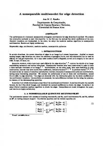
However, classical edge detectors usually fail to handle imanges with strong noise, as shown in Fig. 1.1. Noise is unpredictable contamination on the original image. usually introduced by the transmission or compression of the image.

(a) Lena image

(b) Edges using Canny detector

(c) Lena image with noise (d) Edges from the image with noise Fig. 1.1: Impact of noise on edge detection

It is

1.4 Edge detector with pre-smoothing

4

There are various kinds of noise, but the most widely studied two kinds are white noise and “ salt and pepper” noise. Fig. 1.1 shows the dramatic difference between the result of edge detection from two similar images, with the later one affected by some white noise.

1.4

Edge detector with pre-smoothing

To reduce the influence of noise, two techniques were developed from 1979 to 1984. Marr, et al. suggested filtering the images with the Gaussian before edge detection ( [28]-[30] ); Hueckel [22] and Haralick [33] proposed to approximate the image with a smooth function. The weakness of the above approaches is that the optimal result may not be obtained by using a fixed operator. Canny [4] developed a computational approach to edge detection in 1991. He derived that an optimal detector can be approximated by the first derivative of a Gaussian.

1.5 Development of wavelet analysis

1.5

5

Development of wavelet analysis

The concept of wavelet analysis has been developed since the late 1980’s. However, its idea can be traced back to the Littlewood-Paley technique and Calderón-Zygmund theory [25] in harmonic analysis. Wavelet analysis is a powerful tool for time-frequency analysis. Fourier analysis is also a good tool for frequency analysis, but it can only provide global frequency information, which is independent of time. Hence, with Fourier analysis, it is impossible to describe the local properties of functions in terms of their spectral properties, which can be viewed as an expression of the Heisenberg uncertainty principle [13]. In many applied areas like digital signal processing, time-frequency analysis is critical. That is, we want to know the frequency properties of a function in a local time interval. Engineers and mathematicians developed analytic methods that were adapted to these problems, therefore avoiding the inherent difficulties in classical Fourier analysis. For this purpose, Dennis Gabor [34] introduced a “ sliding-window” technique. He used a Gaussian function g as a “ window” function, and then calculated the Fourier transform of a function in the “ sliding window”. The analyzing function is ga,b (x) = eiax g(x − b), a, b ∈ R. The Gabor transform is useful for time-frequency analysis.

The Gabor transform was

later generalized to the windowed Fourier transform in which g is replaced by a “ timelocal” function called the “ window” function. However, this analyzing function has the disadvantage that the spatial resolution is limited by the fixed size of the Gaussian envelope [13].

1.5 Development of wavelet analysis

6

In 1985, Yves Meyer ( [23], [24] ) discovered that one could obtain orthonormal bases for L2 (R) of the type ψ j,k (x) = 2j/2 ψ(2j x − k),

j, k ∈ Z,

and that the expression f=

X

< f, ψ j,k > ψ j,k ,

j,k∈Z

for decomposing a function into these orthonormal wavelets converged in many function spaces. The most preeminent books on wavelets are those of Meyer ( [23], [24] ) and Daubechies [8]. Meyer focuses on mathematical applications of wavelet theory in harmonic analysis; Daubechies gives a thorough presentation of techniques for constructing wavelet bases with desired properties, along with a variety of methods for mathematical signal analysis [14]. A particular example of an orthonormal wavelet system was introduced by Alfred Haar [35]. However, the Haar wavelets are discontinuous and therefore poorly localized in frequency. Stéphane Mallat ( [36], [37] ) made a decisive step in the theory of wavelets in 1987 when he proposed a fast algorithm for the computation of wavelet coefficients. He proposed the pyramidal schemes that decompose signals into subbands. These techniques can be traced back to the 1970s when they were developed to reduce quantization noise [39]. The framework that unifies these algorithms and the theory of wavelets is the concept of a multi-resolution analysis (MRA). An MRA is an increasing sequence of closed, nested subspaces {Vj }j∈Z that tends to L2 (R) as j increases. Vj is obtained from Vj+1 by a dilation of factor 2. V0 is spanned by a function φ that satisfies

1.6 Edge detector using wavelets

φ(x) = 2

X

hn φ(2x − n).

7

(1.1)

Equation (1.1) is called the “ two-scale equation”, and it plays an essential role in the theory of wavelet bases. In chapter three, Mallat’s wavelet theories are discussed in more detail. In 1997, Chui and Wang [11] further discussed the asymptotically optimal timefrequency localization by scaling functions and wavelets. In their paper they proved the convergence of the time-frequency window sizes of cardinal polynomial B-wavelets, which are used in Mallat’s algorithm and are important in many other wavelet applications.

1.6

Edge detector using wavelets

Now that we have talked briefly about the development of edge detection techniques and wavelet theories, we next discuss how they are related. Edges in images can be mathematically defined as local singularities. Until recently, the Fourier transforms was the main mathematical tool for analyzing singularities. However, the Fourier transform is global and not well adapted to local singularities. It is hard to find the location and spatial distribution of singularities with Fourier transforms. Wavelet analysis is a local analysis, it is especially suitable for time-frequency analysis [1], which is essential for singularity detection. This was a major motivation for the study of the wavelet transform in mathematics and in applied domains. With the growth of wavelet theory, the wavelet transforms have been found to be remarkable mathematical tools to analyze the singularities including the edges, and further, to detect them effectively. This idea is similar to that of John Canny [4]. The Canny

1.7 The purpose of this paper and its organization

8

approach selects a Gaussian function as a smoothing function θ; while the wavelet-based approach chooses a wavelet function to be θ0 .

Mallat, Hwang, and Zhong ( [5], [6] )

proved that the maxima of the wavelet transform modulus can detect the location of the irregular structures. Further, a numerical procedure to calculate their Lipschitz exponents has been provided. One and two-dimensional signals can be reconstructed, with a good approximation, from the local maxima of their wavelet transform modulus. The wavelet transform characterizes the local regularity of signals by decomposing signals into elementary building blocks that are well localized both in space and frequency. This not only explains the underlying mechanism of classical edge detectors, but also indicates a way of constructing optimal edge detectors under specific working conditions.

1.7

The purpose of this paper and its organization

The purpose of this paper is to explain the working mechanism of edge detectors from the point of view of wavelet transforms and to develop a new wavelet-based multi-level edge detection method. Chapter two is an introduction to wavelet transforms.

The relationship between

wavelet transforms and edge detection is discussed in detail in chapter three.

In light

of Mallat’s wavelet theory, we are able to construct a universal wavelet model for edge detection. After a brief review of some classical edge detectors in chapter four, we go on in chapter five to interpret those edge detectors from the point of view of wavelet transforms. Finally, in chapter six, we developed a multiscale wavelet model for edge detection.

1.8 Some notation

9

The fast algorithm suggested by Mallat, et al. ( [5], [6] ) is based on a dyadic scale, which makes it reach large scales quickly. However, when dealing with noisy images, the noise level (SNR) is sensitive to the change of scales. A dyadic sequence of scales cannot always optimally adapt to the effect of noise. With the cascade algorithm developed in chapter four, one can quickly reach a scale of the wavelet that adapts to the scale of signals and the noise level, which minimizes the effect of noise on edge detection.

1.8

Some notation

Before we begin the discussion of wavelet transform, we introduce some notation. L2 (R) denotes the Hilbert space of measurable functions, such that Z +∞ |f (x)|2 dx < +∞.

(1.2)

−∞

For f ∈ L2 (R) , the norm, ||f || , is given by Z +∞ 2 |f (x)|2 dx. ||f || =

(1.3)

−∞

The convolution of two functions f (x) ∈ L2 (R) and g(x) ∈ L2 (R) is denoted by Z +∞ f (u)g(x − u)du. (1.4) f ∗ g(x) = −∞

The Fourier transform of a function f (x) is defined by fb(ω) = lim

N →∞

Z

N

f (x)e−iωx dx,

(1.5)

−N

and the s-dilation of f (x) is defined by

1 ³x´ fs (x) = f , s > 0. s s

(1.6)

1.8 Some notation

10

Similarly, let L2 (R2 ) be the Hilbert space of two-dimensional square-integrable functions. The norm of f ∈ L2 (R2 ) is given by Z +∞ Z 2 ||f || = −∞

+∞

−∞

|f (x, y)|2 dxdy,

(1.7)

and the Fourier transform of f ∈ L2 (R2 ) is defined by fb(ω x , ωy ) =

Z

+∞

−∞

Z

+∞

f (x, y) e−i(ωx x+ωy y) dxdy.

(1.8)

−∞

For any function f ∈ L2 (R2 ) , fs (x, y) denotes the s-dilation of f (x, y) fs (x, y) =

1 ³x y ´ , , s > 0. f s2 s s

(1.9)

Chapter 2 Introduction to Wavelet Transforms

2.1

Continuous wavelet transforms

We know that the Fourier transform of a signal f (t) is defined as fb(ω) =

Z

∞

f (t)e−iωt dt.

−∞

Since e−iωt is globally supported and not in L2 , Fourier analysis is global in nature, which makes it not suitable for detecting local singularities. To obtain the approximate frequency contents of a signal f (t) in the neighborhood of some desired location t = b, we can window the function using an appropriate window function φ(t) to produce the windowed function fb (t) = f (t)φ(t − b) and then take the Fourier transform of fb (t). This is called the short-time Fourier transform (STFT). It can be defined at the location (b, ξ) in the time-frequency plane as Gφ f (b, ξ) =

Z

∞

f (t)φb,ξ (t)dt

(2.10)

−∞

where φb,ξ (t) = φ(t − b)eiξt .

(2.11)

One can recover the time function f (t) by taking the inverse Fourier transform of Gφ f (b, ξ), then multiply by φ(t − b) and integrate with respect to b: Z ∞ Z ∞ 1 iξt f (t) = dξe Gφ f (b, ξ)φ(t − b)db 2π ||φ||2 −∞ −∞

11

(2.12)

2.1 Continuous wavelet transforms

If we use the Gaussian function as the window function, i.e., φ(t) =

12

2

t 1 − 4α e 2πα

(α >

0), the transform is called the Gabor transform [34]. If we use a dilated and translated wavelet function as φb,ξ (t), i.e., φb,ξ (t) = ψ b,ξ (t), the transform is a continuous wavelet transform. Definition 1 The continuous wavelet transform(CWT) of a function f (t) ∈ L2 with respect to some analyzing wavelet ψ is defined as Z

Wψ f (b, a) =

∞

f (t)ψ b,a (t)dt,

−∞

where 1 ψ b,a (t) = √ ψ a

µ

¶ t−b , a

a > 0,

(2.13)

and ψ(t) satisfies the following condition: b ψ(0) =

Z

∞

ψ(t)dt = 0.

(2.14)

−∞

In addition to satisfying (2.14), a wavelet is sometimes constructed such that it has vanishing moments of higher order. A wavelet is said to have vanishing moments of order m if

Z

∞

tp ψ(t)dt = 0,

−∞

p = 0, ..., m − 1.

(2.15)

We often derive ψ(t) from the derivative of a smoothing function φ(t) ∈ L2 (R), Z ∞ φ(t)dt = 1 −∞

ψ(t) =

dφ . dt

2.1 Continuous wavelet transforms

13

Theorem 1 Let φ(t) ∈ L2 (R) be a smoothing function that is n times diﬀerentiable. Let ψ p (t) be the pth derivative of φ(t), i.e. ψ p (t) =

dp φ(t) , p < n, dtp

(2.16)

then ψ p (t) has vanishing moments of order p. Proof. Since

Z

∞

−∞

ψ(t)dt = lim φ(t) − lim φ(t) = 0 t→∞

t→−∞

(2.17)

According to (2.14) and (2.15), ψ(t) is a wavelet with vanishing moments of order 1. Assume that ψ p−1 (t) has vanishing moments of order p − 1, i.e. Z ∞ tp−2 ψ p−1 (t)dt = 0,

(2.18)

−∞

Then Z

∞

−∞

p−1

t

ψ p (t)dt =

Z

∞

−∞

p−1

= t

= 0.

(2.19)

tp−1 dψ p−1 (t) ¯∞ ψ p−1 (t)¯−∞ − (p − 1)

Z

∞

tp−2 ψ p−1 (t)dt

−∞

Thus by induction ψ p (t) has vanishing moments of order p.

Similar to STFT, the inverse wavelet transform involves a two-dimensional integration over the scale parameter a and the translation parameter b : Z ∞ Z ∞ 1 1 db (Wψ f (b, a)) ψ b,a (t) da, f (t) = 2 Cψ −∞ −∞ a

(2.20)

2.2 Multi-resolution analysis

where Cψ is a constant given by Cψ =

Z

∞

−∞

¯2 ¯ ¯ ¯b ¯ψ (ω)¯ |ω|

dω < ∞.

14

(2.21)

The condition (2.21), known as the admissibility condition, restricts the class of functions that can be wavelets. It actually implies (2.14) [1].

2.2

Multi-resolution analysis

A careful choice of the mother wavelet φ is crucial to the Fast Wavelet Transform, (FWT). The mother wavelet should in a certain way “ reproduce itself” when it is subject to scaling. More specifically, the mother wavelet ψ satisfies a linear identity having the following structure: D2 φ(t) =

n X k=0

ck φ(t − k),

(2.22)

where D2 is a scaling operation such that D2 φ(t) = φ( 2t ). In another words, φj (t) forms an MRA.

Definition 2 A multi-resolution analysis, abbreviated MRA, is constituted by the following ingredients (a)-(c). (a) A bilateral sequence (Vj |j ∈ Z) of closed subspaces of L2 . These Vj are ordered by inclusion, ... ⊂ V2 ⊂ V1 ⊂ V0 ⊂ V−1 ⊂ ... ⊂ Vj ⊂ Vj−1 ⊂ ... ⊂ L2

(2.23)

2.2 Multi-resolution analysis

15

(smaller values of j correspond to larger spaces Vj ), with ∩j Vj = {0} (seperation axiom), ∪j Vj = L2

(completeness axiom).

(2.24) (2.25)

(b) The Vj are connected to each other by a rigid scaling property: Vj+1 = D2 (Vj )

∀j ∈ Z

(2.26)

(c) V0 contains one basis vector per base step 1, i.e., there is a function φ ∈ L2 ∩ L1 such that its translates (φ (· − k) |k ∈ Z) form an orthonormal basis of V0 . The function φ is commonly called the scaling function of the MRA and it determines V0 : ( ) X X V0 = f ∈ L2 |f (t) = ck φ(t − k), |ck |2 < ∞ k

k

(2.27)

2.3 Scale of a wavelet function

2.3

16

Scale of a wavelet function

First, we consider some special characteristics of Gaussian filters. A Gaussian function through a Gaussian filter is still a Gaussian function, but with a dilated variance.

Let

gσ (x, y) be a normalized Gaussian function with variance σ 2 ,then (gσ1 ∗ gσ2 )(x, y) Z ∞Z ∞ = gσ1 (x − h, y − k)gσ2 (h, k)dhdk −∞

−∞

1 = 2 4π σ 21 σ 22 1 = 2 4π σ 21 σ 22

=

1 4π 2 σ 21 σ 22

Z

∞

−∞

Z

∞

−∞

Z

∞

−∞

Z

∞

(x−h)2 +(y−k)2 2σ 2 1

−

e

−∞

Z

∞

∞

2 2σ 2 1 σ2

e

Ã

σ2 x h− 2 2 2 σ1 +σ 2

!2

−

x2 +y 2

(

(

)

)

σ2 σ2 2 21 22 σ 1 +σ 2

e Z

x2 +y 2

dhdk

Ã !2 2 2 2 σ2 σ2 x 1 σ 2 x +y + k− 2 2 2 + σ 1 +σ 2 2 2 2 σ2 1 +σ 2

−∞

− 1 2 2 2(σ 2 1 +σ 2 ) = e 4π 2 σ 21 σ 22

dhdk

(σ21 +σ22 )h2 −2σ22 hx+σ22 x2 +(σ21 +σ22 )k2 −2σ22 ky+σ22 y2

−

−∞

Z

2 +k2 2σ 2 2

−h

e

∞

−∞

Z

∞

−

Ã

Ã !2 σ2 y + k− 2 2 2 σ 1 +σ 2 σ2 σ2 1 2 2 2 σ 1 +σ 2 2

σ2 x h− 2 2 2 σ 1 +σ 2

e

dhdk !2

dhdk

−∞

− 1 2 2 2(σ 2 1 +σ 2 ) e = 2π(σ 21 + σ 22 )

= g√σ2 +σ2 (x, y) 1

(2.28)

2

Now, we consider a special class of wavelets, which can be defined as the derivative of a smoothing function, i.e., ψ(x, y) = where

RR

R2

∂ φ(x, y), ∂x

φ(x, y) = 1. If the Gaussian is used as the smoothing function, this class of

wavelets is called a Gaussian wavelet. From (2.28), we can develop a cascade algorithm

2.4 Approximation of the Gaussian filter with B-splines

17

to find the wavelet transform of f (x, y) on a series of scales. W 1 f (ns, x, y) = ψns ∗ f (x, y) ∂φns ∗ f (x, y) ∂x ∂(φ(n−1)s ∗ φs ) ∗ f (x, y) = ∂x ∂(φ(n−1)s ∗ f ) ∗ φs (x, y) = ∂x =

= W 1 f ((n − 1)s, x, y) ∗ φs (x, y)

(2.29)

Thus, for any integer n > 1, W 1 f (ns, x, y) = φs ∗ ... ∗ φs ∗W 1 f (s, x, y) | {z }

(2.30)

W 2 f (ns, x, y) = φs ∗ ... ∗ φs ∗W 2 f (s, x, y) | {z }

(2.31)

n−1

Similarly,

n−1

2.4

Approximation of the Gaussian filter with B-splines

Next, we use cardinal B-splines to approximate the Gaussian filter. Definition 3 The cardinal B-spline of order m, denoted by Nm (x), is inductively defined by the multi-convolution of the box function: N1 (x) = B(x) =

½

1, 0 ≤ x ≤ 1; , 0, otherwise

Nm (x) = Nm−1 ∗ N1 (x)


18

i.e. m z }| { Nm (x) = N1 ∗ N1 ∗ · · · ∗ N1 (x)

(2.32)

Although the cardinal B-spline of order 1 is not an accurate approximation of a Gaussian function, it has been shown in [38] that the cardinal B-spline of order n asymptotically converges to a Gaussian function φn (x) as n goes to infinity. φn (x) ≈ Nn (x), n−2

z }| { = N1 ∗ ... ∗ N1 (x)

(2.33)

where Nn (x) is a B-spline with support n.

We now introduce a cascade algorithm that detects edges continuously on all integer scales. Let H(x) be the Haar wavelet

⎧ ⎨ −1, 0 ≤ x < 12 ; 1, 12 ≤ x ≤ 1; H(x) = ⎩ 0, otherwise. ψ 1 (x) ≈ H(x),

where ψ 1 (x) is the Gaussian wavelet of scale 1. Thus the Gaussian wavelet at integer scale n > 2 can be approximated as n−2

z }| { ψ n (x) ≈ N1 ∗ ... ∗ N1 ∗H(x) = Nn−2 ∗ H(x).


19

We can easily expand this method to calculate the wavelet transform of a discrete 2-D image f (x, y), by defining B(x, y), H 1 (x, y) and H 2 (x, y) as follows: ½ 1, 0 ≤ x ≤ 1, 0 ≤ y ≤ 1; N1 (x, y) = B(x, y) = 0, otherwise. ⎧ ⎨ −1, 0 ≤ x < 12 , 0 ≤ y ≤ 1; 1, 1 ≤ x ≤ 1, 0 ≤ y ≤ 1; H 1 (x, y) = ⎩ 2 0, otherwise. ⎧ ⎨ −1, 0 ≤ x ≤ 1, 0 ≤ y < 12 ; 1, 0 ≤ x ≤ 1, 12 ≤ y ≤ 1; H 2 (x, y) = ⎩ 0, otherwise. And thereby,

n−2

(2.34)

z }| { W 1 f (n, x, y) ≈ N1 ∗ ... ∗ N1 ∗H 1 ∗ f (x, y); n−2

z }| { W 2 f (n, x, y) ≈ N1 ∗ ... ∗ N1 ∗H 2 ∗ f (x, y).

We use (2.34) to calculate the horizental and vertical wavelet transform at scale n. In practice, we sometimes need the wavelet transform with a rotated direction. To do this, we define the approximation for a rotated wavelet: ⎧ ⎨ −1, 0 ≤ x < y ≤ 1; 3 1, 0 ≤ y ≤ x ≤ 1; H (x, y) = ⎩ 0, otherwise. ⎧ ⎨ −1, 0 ≤ x < −y ≤ 1; 4 1, 0 ≤ −y ≤ x ≤ 1; H (x, y) = ⎩ 0, otherwise. Similarly,


20

n−2

z }| { W 3 f (n, x, y) ≈ N1 ∗ ... ∗ N1 ∗H 3 ∗ f (x, y);

(2.35)

n−2

z }| { W 4 f (n, x, y) ≈ N1 ∗ ... ∗ N1 ∗H 4 ∗ f (x, y).

Fig. 2.1 shows how the Gaussian wavelet is approximated by B-spline. Each

(a)

(b)

(c)

(d)

(e) (f) Fig. 2.1: (a),(b): One iteration; (c),(d): 10 iterations; (e),(f): 20 iterations

(2.36)

2.5 Wavelets with vanishing moments of higher order

21

iteration of convolution with N1 raise the order of the B-spline by 1.

2.5

Wavelets with vanishing moments of higher order

Up to this point, only the first-degree derivative of the smoothing function is used as a wavelet. This is usually sufficient for edge detection of normal images. But in some special cases where we wish to detect discontinuities that are less noticeable, wavelets defined by higher degree derivatives may be used. In such cases, we can simply repeat the convolution with H. Each time we do the convolution with H, we increase the order of the derivative by one, and thus increase the order of vanishing moments by 1. This can easily be shown as follows: dk φn dxk ¢ dk ¡ = ∗ φ φ n−1 1 dxk dk−1 φn−1 dφ1 ∗ , (k < n). = dxk−1 dx

ψ (k) =

(2.37)

Thus, by induction and from (2.32), (2.33),

ψ (k)

k z }| { dφ1 dφ1 ∗ ... ∗ = φn−k ∗ dx dx

In 2-D, W(k) f (n, x, y) = ψ (k) ∗ f (x, y) n−k−1

k

z }| { z }| { ≈ N1 ∗ ... ∗ N1 ∗ H ∗ ... ∗ H ∗f (x).

(2.38)

2.5 Wavelets with vanishing moments of higher order

22

Fig. 2.2 shows an approximation of a wavelet with vanishing moments of order two.

(a) (b) Fig. 2.2: Approximation by 30 iterations of convolution with N1 for a wavelet with vanishing moments of order two

Chapter 3 Edge Detection Using Wavelets A remarkable property of the wavelet transform is its ability to characterize the local regularity of functions.

For an image f (x, y), its edges correspond to singularities of

f (x, y), and thus are related to the local maxima of the wavelet transform modulus. Therefore, the wavelet transform is an effective method for edge detection.

3.1

General rules of edge detection

Edge detectors are modified gradient operators. Since an edge is characterized by having a gradient of large magnitude, edge detectors are approximations of gradient operators. Because noise influences the accuracy of the computation of gradients, usually an edge detector is a combination of a smoothing filter and a gradient operator. An image is first smoothed by the smoothing filter and then its gradient is computed by the gradient operator. The 2-norm of the gradient is k∇f k2 =

p 2 fx + fy2 . In order to simplify computation,

in image processing we often use the 1-norm k∇f k1 = |fx | + |fy | instead. Their discrete forms are k∇f k2 =

p (f (i − 1, j) − f (i + 1, j))2 + (f (i, j − 1) − f (i + 1, j))2

k∇f k1 =

1 1 |f (i − 1, j) − f (i + 1, j)| + |f (i, j − 1) − f (i, j + 1)| 2 2

and

respectively.

23

(3.39)

(3.40)

3.2 Mallat0 s wavelet

24

In image processing, the following two ways are used to define edges. (1) Local maxima definition. Let f (x, y) ∈ H 2 (Ω). A point (x, y) ∈ Ω0 is called an edge point of the image f (x, y), if k∇f k has a (strictly) local maximum at (x, y), i.e., k∇f (x, y)k > k∇f (x, y)k in a neighborhood of (x, y). An edge curve in an image is a continuous curve on which all points are edge points. The set of all edge points of f (x, y) is called an edge image of f (x, y). (2) Threshold definition. Let f (x, y) ∈ H 2 (Ω). Assume that max k∇f (x, y)k = M.

(x,y)∈Ω

(3.41)

Choose K, 0 < K < M, as the edge threshold. If k∇f (x, y)k ≥ K, then (x, y) is called an edge point of f (x, y).

3.2

Mallat0s wavelet

We first define a smoothing function φ(x), then we build the wavelet ψ(x), which is associated with φ(x). We know that the Fourier transform of the smoothing function φ(x) can be written as an infinite product φ(ω) = e−i$ω

+∞ Y

H(2−p ω)

(3.42)

p=1

where H(ω) is a 2π periodic differentiable function such that |H(ω)|2 + |H(ω + π)|2 ≤ 1 and |H(0)| = 1 b We define a wavelet ψ(x) whose Fourier transform ψ(ω) is given by

(3.43)

3.2 Mallat0 s wavelet

b b ψ(2ω) = e−i$ω G(ω)φ(ω),

25

(3.44)

where G(ω) is a 2π periodic function.

Let the smoothing function θ(x) be such that ψ(x) is the first-order derivative of θ(x). A family of 2π periodic functions H(ω) and G(ω), that satisfy these constrains, is given by H(ω) = eiω/2 (cos(ω/2))2n+1 ,

(3.45)

G(ω) = 4ieiω/2 sin(ω/2),

(3.46)

From (3.45), we derive ¶2n+1 sin(ω/2) , ω/2 µ ¶2n+2 sin(ω/4) b ψ(ω) = iw . ω/4 b φ(ω) =

µ

The Fourier transform b θ(ω) of the primitive is therefore ¶2n+2 µ sin(ω/4) b θ(ω) = ω/4

(3.47) (3.48)

(3.49)

Equations (3.47), (3.49) prove that ψ(x) is a quadratic spline with compact support, whereas θ(x) is a cubic spline whose integral is equal to 1, as shown in Fig. 3.1.

(a) quadratic spline (b) cubic spline Fig. 3.1: B-splines defined in Mallat0 s wavelet. Now the wavelet is expanded to 2-D. Define

3.3 Construction of wavelets for edge detection

ψ 1 (x, y) = 2ψ(x)φ(2y)and ψ 2 (x, y) = 2φ(2x)ψ(y). Since ψ(x) =

dθ(x) , dx

26

(3.50)

these two wavelets can be rewritten as

ψ 1 (x, y) =

∂θ1 (x, y) ∂θ2 (x, y) and ψ 2 (x, y) = , with ∂x ∂y

(3.51)

θ1 (x, y) = 2θ(x)φ(2y)and θ2 (x, y) = 2φ(2x)θ(y). The functions θ1 (x, y) and θ2 (x, y) are numerically close enough so that they can be considered to be equal to a single function θ(x, y) in a first approximation.

3.3

Construction of wavelets for edge detection

We assume the smoothing function θ(x) is twice differentiable and define, respectively, ψ a (x) and ψ b (x) as the first- and second-order derivatives of θ(x) ψ a (x) =

dθ(x) d2 θ(x) and ψ b (x) = . dx dx2

(3.52)

By the definition in (2.14), the functions ψ a (x) and ψ b (x) can be considered to be wavelets because their integral is equal to 0. Z Z +∞ a ψ (x)dx = 0and −∞

+∞

ψ b (x)dx = 0

−∞

A wavelet transform is computed by convolving the signal with a dilated wavelet. The wavelet transform of f (x) at the scale s and position x, computed with respect to the wavelet ψ a (x), is defined by Wsa f (x) = f ∗ ψ as (x).

(3.53)


27

The wavelet transform of f (x) with respect to ψ b (x) is Wsb f (x) = f ∗ ψ bs (x).

(3.54)

d dθs )(x) = s (f ∗ θs )(x), and dx dx 2 d θs d2 Wsb f (x) = f ∗ (s2 2 )(x) = s2 2 (f ∗ θs )(x). dx dx

(3.55)

It follows that Wsa f (x) = f ∗ (s

(3.56)

Therefore, the wavelet transforms Wsa f (x) and Wsb f (x) are, respectively, the first and second derivative of the signal smoothed at the scale s. The local extrema of Wsa f (x) thus correspond to the zeros of Wsb f (x) and to the inflection points of f ∗ θs (x). Let ψ 1s (x, y) =

1 ψ (x, y) s2 1 s s

and ψ 2s (x, y) =

1 ψ ( x , y ). s2 2 s s

Let f (x, y) ∈ L2 (R2 ). The

wavelet transform of f (x, y) at the scale s has two components defined by Ws1 f (x, y) = f ∗ ψ 1s (x, y)and Ws2 f (x, y) = f ∗ ψ 2s (x, y). It is straight forward that µ 1 ¶ µ Ws f (x, y) =s Ws2 f (x, y)

∂ (f ∂x ∂ (f ∂y

∗ θs )(x, y) ∗ θs )(x, y)

¶

= s∇(f ∗ θs )(x, y)

(3.57)

(3.58)

Hence, edge points can be located from the two components, Ws1 f (x, y) and Ws2 f (x, y), of the wavelet transform. We choose the Gaussian as the smoothing function for Mallat’s wavelet. i.e. θ(x, y) =

1 − (x2 +y2 2 ) e 2σ . 2πσ 2

Thus, the corresponding wavelet ψ 1 (x, y) and ψ 2 (x, y) is given by ψ 1 (x, y) =

∂θ x − (x2 +y2 2 ) e 2σ ; =− ∂x 2πσ 4

(3.59)


ψ 2 (x, y) =

y − (x2 +y2 2 ) ∂θ =− e 2σ . ∂y 2πσ 4

28

(3.60)

Higher degree differentiations of θ also comply with the definition of wavelets in (2.14). ∂ 2θ xy − (x2 +y2 2 ) = e 2σ ; ∂x∂y 2πσ 6 ∂ 4θ (σ 2 − x2 ) (σ 2 − y 2 ) − (x2 +y2 2 ) e 2σ . = ∂ 2 x∂ 2 y 2πσ 10

(3.61) (3.62)

3.4 Edge detection with wavelet maxima

3.4

29

Edge detection with wavelet maxima

In a signal, there are usually four kinds of edges, which can be indicated in one dimension as in Fig. 3.2(a).

f (x) (a) W f(21 , x) W f(22 , x) W f(23 , x) W f(24 , x) W f(25 , x) W f(26 , x) (b) 21 22 Scales 23 24 25 26 (c) Fig. 3.2: Wavelet transform of different types of edges throughout scales : (a) Original signal; (b) wavelet transform computed up to the scale 26 ; (c)At each scale, each Dirac indicates the position of a modulus location.


30

The edges between 0 and 100 are step edges; The edge between 100 and 200 is a smoothed step edge; The edge between 200 and 300 is a Dirac edge; and the edges between 350 and 650 are fractal edges. Fig. 3.2(b) shows the wavelet transform of this signal on different edges in dyadic scales. Fig. 3.2(c) shows the modulus maxima which indicates the location of the edges. By taking the wavelet transform, we can locate all four kinds of edges. Here, we will explain the reason by presenting some theorems. In an image, all edges are not created equal. Some are more significant, and some are blurred and insignificant. The edges of more significance are usually more important and more likely to be kept intact by wavelet transforms. The insignificant edges are sometimes introduced by noise and preferably removed by wavelet transforms. In mathematics, the sharpness of an edge can be described with Lipschitz exponent. We will later show that local Lipschitz regularity can be efficiently measured by wavelet transforms. We first introduce the definition of Lipschitz exponent in 1-D. Definition 4

• Let n be a positive integer and n ≤ α ≤ n + 1. A function f (x) is said to be Lipschitz α, at x0 , if and only if there exists two constants A and h0 > 0, and a polynomial of order n, Pn (x), such that for h < h0 |f (x0 + h) − Pn (h)| ≤ A |h|α .

(3.63)

• the function f (x) is uniformly Lipschitz α over the interval (a, b), if and only if there exists a constant A and for any x0 ∈ (a, b), there exists a polynomial of order n, Pn (h), such that equation (3.63) is satisfied if x0 + h ∈ (a, b).


31

• We call Lipschitz regularity of f (x) at x0 , the superior bound of all values α at x0 . • We say that a function is singular at x0 , if it is not Lipschitz 1 at x0 . The definition is now extended to 2-D. Definition 5 Let 0 ≤ α ≤ 1. For any ε > 0, the function f (x, y) is called uniformly Lipschitz α on the interval of (a + ε, b − ε) × (c + ε, d − ε), if there exists a constant Aε , such that, for (x, y) ∈ (a + ε, b − ε) × (c + ε, d − ε), h2 + k2 < ε2 , the following holds: α

|f (x + h, y + k) − f (x, y)| ≤ Aε (h2 + k 2 ) 2 .

(3.64)

We refer to the Lipschitz uniform regularity of f (x, y) as the upper bound α0 of all α such that f (x, y) is uniformly Lipschitz α. The local Lipschitz regularity of a function f (x, y) is estimated from the evolution across scales of both |Ws1 f (x, y)| and |Ws2 f (x, y)|. The value of each of these components is bounded by q Mf (s, x, y) = |Ws1 f (x, y)|2 + |Ws2 f (x, y)|2 ,

(3.65)

where the function Mf(s, x, y) is called he modulus of the wavelet transform at the scale 2j . It is proportional to the modulus of the gradient vector ∇ (f ∗ θ2j ) (x, y). Theorem 2 Let f (x, y) ∈ L2 (R2 ) and 0 < α < 1. For any ε > 0, f (x, y) is uniformly Lipschitz α over (a + ε, b − ε) × (c + ε, d − ε), if and only if for any ε > 0 there exists a constant Aε such that for (x, y) ∈ (a + ε, b − ε) × (c + ε, d − ε) and any scale s > 0 |Mf (s, x, y)| ≤ Aε sα .

(3.66)


Proof.

32

For the ”only if” part, since f (x, y) ∈ L2 ∩ L1 (R2 ) is uniformly Lipschitz

α over (a + ε, b − ε) × (c + ε, d − ε), there exists an A1 > 0 such that, given any scale s > 0, for (x, y) ∈ (a + ε, b − ε) × (c + ε, d − ε) and any scale h > 0, k > 0, h2 + k2 < min(ε2 , s2 ) α

|f (x + h, y + k) − f (x, y)| ≤ A1 (h2 + k2 ) 2 . According to the definition of ψ 1s (x, y) , for any given (x, y), Z +∞ Z +∞ f (x, y)ψ 1s (h, k)dhdk = 0 −∞

ψ 1s (x, y) = Thus with (3.68), we have

(3.67)

(3.68)

−∞

C 1 1 x y ´ ψ ( , )< ³ 2 2 2 1+ α s s s 2 s2 1 + ( x s+y ) 2

(3.69)

¯ ¯ ¯ ¯ 1 ¯W f (s, x, y)¯ = ¯(ψ 1s ∗ f )(x, y)¯ ¯Z +∞ Z +∞ ¯ ¯ ¯ 1 ¯ = ¯ f (x + h, y + k)ψ s (h, k)dhdk¯¯ −∞ ¯Z−∞ ¯ Z ¯ +∞ +∞ ¯ 1 = ¯¯ (f (x + h, y + k) − f (x, y)) ψ s (h, k)dhdk¯¯ −∞ −∞ Z +∞ Z +∞ ¯ ¯ ≤ |(f (x + h, y + k) − f (x, y))| ¯ψ 1s (h, k)¯ dhdk −∞

−∞

(3.70)

Let Ω = {(h, k) | h2 + k2 < s2 }, thus, we apply (3.67) inside the neighborhood of Ω, Z Z ¯ ¯ |(f (x + h, y + k) − f (x, y))| ¯ψ 1s (h, k)¯ dhdk Z ZΩ ¯ α ¯ A1 (h2 + k 2 ) 2 ¯ψ 1s (h, k)¯ dhdk ≤ Ω

¯¯ ¯¯ ≤ A1 ¯¯ψ 1s ¯¯ sα = A1 sα

(3.71)


33

and we use the decay condition (3.69) of the wavelet outside Ω, Z Z ¯ ¯ |(f (x + h, y + k) − f (x, y))| ¯ψ 1s (h, k)¯ dhdk 2 Z ZR \Ω 1 C1 ¡ ≤ 2 2 1+ α ¢dhdk h s2 1 + ( s+k ) 2 R2 \Ω 2 Z Z 1 = sα C1 α dhdk α 2 s + (h + k2 )1+ 2 R2 \Ω (3.72)

≤ sα C2 . From (3.70),(3.71) and (3.72), we have ¯ 1 ¯ Aε α ¯W f (s, x, y)¯ ≤ √ s , 2 √ 2(A1 + C2 ). where Aε = Similarly,

Thus,

¯ 2 ¯ Aε α ¯Ws f (x, y)¯ ≤ √ s . 2 q |Mf (s, x, y)| = |Ws1 f (x, y)|2 + |Ws2 f (x, y)|2 ≤ Aε sα .

Therefore, the ”only if” part is proved.

For the ”if” part, since |Mf (s, x, y)| ≤ Aε sα , ¯ ¯ 1 ¯Ws f (x, y)¯ ≤ Aε sα ,

¯ 2 ¯ ¯Ws f (x, y)¯ ≤ Aε sα .

(3.73)


34

Moreover, according to the definition of the wavelet ψ 1s , Z +∞ Z +∞ Z +∞ ¢ ¡ 1 1 f (x, y) = dh1 dk1 Ws1 f (h1 , k1 ) ψ 1s1 (x + h1 , y + k1 )ds1 , (3.74) Cψ −∞ −∞ 0

where Cψ is a constant and is given by Z +∞ Z +∞ c1 ψ s (ωx , ω y ) Cψ = 1 dω x dω y < ∞. 2 2 −∞ −∞ (ω x + ω y ) 2 Therefore, from (3.73) and (3.74), we have

|f (x + h, y + k) − f (x, y)| Z +∞ Z +∞ 1 ≤ dh1 dk1 Cψ −∞ −∞ Z +∞ ¯ ¯ Aε sα ¯ψ 1s1 (x + h + h1 , y + k + k1 ) − ψ 1s1 (x + h1 , y + k1 )¯ ds1 0

Since s is arbitrary, without loss of generality, we choose s such that s2 = h2 +k2 . Using the mean value theorem, Z +∞ Z +∞ dh1 dk1 −∞ −∞ Z +∞ ¯ ¯ Aε sα ¯ψ 1s1 (x + h + h1 , y + k + k1 ) − ψ 1s1 (x + h1 , y + k1 )¯ ds1 s

α

≤ Aε s

Z

+∞

⎛s

⎜ ⎜ sup ⎜ ⎝ 2

1+

µ³ 2

≤ Aε (h + k ) Furthermore,

1

(h2 + k2 ) 2 C ds1 s31

α 2

Z

1 h1 +h s1

Z

s

´2

+∞

+

³

k1 +k s1

+∞

−∞

Z

+∞

−∞

´2 ¶1+α ,

⎟ ⎟ ³ 2 2 ´1+α ⎟ dh1 dk1 h1 +k1 ⎠ 1

1+

⎞

α C1 ds1 ≤ Aε C2 (h2 + k2 ) 2 3 s1

s21


Z

+∞

Z−∞ s

dh1

Z

35

+∞

dk1

−∞

¯ ¯ Aε sα ¯ψ 1s1 (x + h + h1 , y + k + k1 ) − ψ 1s1 (x + h1 , y + k1 )¯ ds1 Z0 +∞ Z +∞ ≤ dh1 dk1 −∞ −∞ Z s ¢ ¡ Aε sα |ψ 1s1 (x + h + h1 , y + k + k1 )| + |ψ 1s1 (x + h1 , y + k1 )| ds1 0 Z s Z +∞ Z +∞ 2Cs21 α ≤ Aε s dh1 dk1 ds1 2 2 1+ α 2 0 −∞ −∞ 1 + (h1 + k1 ) α

≤ Aε C3 (h2 + k 2 ) 2 Therefore,

α

|f (x + h, y + k) − f (x, y)| ≤ A1 (h2 + k2 ) 2 , where A1 = Aε (C2 + C3 )

Theorem 3 Let n be a positive integer and α ≤ n. Let f (x, y) ∈ L2 (R2 ). If f (x, y) is Lipschitz α at (x0 , y0 ), then there exists a constant A > 0 such that for all point (x, y) in a neighborhood of (x0 , y0 ) and any scale s |Mf (s, x, y)| ≤ A(sα + |x − x0 |α )

(3.75)

Conversely, let α < n be a noninteger value. The function f (x, y) is Lipschitz α at (x0 , y0 ), if the following two conditions hold.

3.5 2-D discrete convolution

36

• There exists some ε > 0 and a constant A such that for all points (x, y) in a neighborhood of (x0 , y0 ) and any scale s |Mf(s, x, y)| ≤ Asε .

(3.76)

• There exists a constant B such that for all points (x, y) in a neighborhood of (x0 , y0 ) and any scale s ! α ¡ 2 2¢ 2 ) + (y − y ) (x − x 0 0 ¢¯ |Mf(s, x, y)| ≤ B sα + 1 ¯ ¡ ¯log (x − x0 )2 + (y − y0 )2 ¯ 2 Ã

(3.77)

Theorem 3 is an extension of Theorem 2 and the proof is similar. Theorem 2 and Theorem 3 prove that the wavelet transform is particularly well adapted to estimating the local regularity of functions. Because edges are singularities characterized by Lipschitz exponent, it is appropriate to locate edges by finding local singularities with the wavelet transform. Fig. 3.3 shows how the coefficients of the wavelet transform change across scales.

3.5

2-D discrete convolution

The convolution of two bi-variate functions f (x, y) and g(x, y) is defined by (f ∗ g)(x, y) =

Z

∞

−∞

Z

∞

−∞

f (x − u, y − v)g(u, v)dudv,

provided that the integral on the right hand side exists. Data from digital images are discrete. So to deal with such image data, we need discrete filters, which can be applied by discrete convolutions. Definition 6 The 2-D discrete convolution of two sequences g and x is a 2-D sequence


37

g ∗ x given by (g ∗ x)(i, j) =

X k,l

g(k, l)x(i − k, j − l), i ∈ Z, j ∈ Z

(3.78)

provided the series in (3.78) is convergent for each i, j ∈ Z. Continuous wavelet models can be converted into discrete edge detectors by discretizing the wavelet with appropriate scales. Suppose the support of a wavelet ψ(x, y) is within an n by n grid (n = 2k + 1, k ∈ Z+ ), then the discrete edge detector defined by the wavelet is g(i, j) =

Z

j+ 12

j− 12

Z

i+ 12

i− 12

ψ(x, y)dxdy, i = −k..k, j = −k..k.

(3.79)


38

(a)

(b) Fig. 3.3: (a) An image with different type of edges. A sample of pixels is taken across the indicated line in the middle; (b) Modulus of the continuous wavelet transform from scale 1 to 26 (brighter color indicates edges).

Chapter 4 Review of Classical Edge Detectors Classical edge detectors use a pre-defined group of edge patterns to match each image segments of a fixed size. 2-D discrete convolutions are used here to find the correlations between the pre-defined edge patterns and the sampled image segment. (f ∗ m)(x, y) =

XX i

j

f (i, j)m(x − i, y − j),

(4.80)

where f is the image and m is the edge pattern defined by m =

m(−1, −1) m(−1, 0) m(−1, 1) m(0, −1) m(0, 0) m(0, 1) , m(1, −1) m(1, 0) m(1, 1)

m(i, j) = 0, if (i, j)is not in the defined grid. These patterns are represented as filters, which are vectors (1-D) or matrices (2-D). For fast performance, usually the dimension of these filters are 1×3 (1-D) or 3×3 (2-D). From the point of view of functions, filters are discrete operators of directional derivatives. Instead of finding the local maxima of the gradient, we set a threshold and consider those points with gradient above the threshold as edge points. Given the source image f (x, y), the edge image E(x, y) is given by E=

p (f ∗ s)2 + (f ∗ t)2 ,

where s and t are two filters of different directions.

39

(4.81)

4.1 Roberts edge detector

4.1

40

Roberts edge detector 0 0 0 s= 0 1 0 0 0 -1

0 0 0 t= 0 1 0 -1 0 0

The edge patterns are shown in Fig. 4.1.

(a)

(b)

Fig. 4.1. Edge patterns for Roberts edge detector: (a) s; (b) t These filters have the shortest support, thus the position of the edges is more accurate. On the other hand, the short support of the filters make it very vulnerable to noise. The edge pattern of this edge detector makes it especially sensitive to edges with a slope around π . 4

Some computer vision programs use the Roberts edge detector to recognize edges of

roads.

4.2

Prewitt edge detector -1 -1 -1 s= 0 0 0 , 1 1 1

-1 0 1 t = -1 0 1 -1 0 1


(a)

(b)

Fig. 4.2: Edge patterns for Prewitt and Sobel edge detectors: (a)s; (b)t These filters have longer support. They differentiate in one direction and average in

4.3 Sobel edge detector

41

the other direction. So the edge detector is less vulnerable to noise. However, the position of the edges might be altered due to the average operation.

4.3

Sobel edge detector -1 -2 -1 s= 0 0 0 , 1 2 1

-1 0 1 t = -2 0 2 -1 0 1

The edge patterns are similar to those of the Prewitt edge detector as shown in Fig. 4.2. These filters are similar to the Prewitt edge detector, but the average operator is more like a Gaussian, which makes it better for removing some white noise.

4.4

Frei-Chen edge detector

A 3×3 subimage b of an image f may be thought of as a vector in R9 . For example, ⎡ ⎤ b0 b4 b3 b2 ⎢ b1 ⎥ ⎥ → b=⎢ b = b5 b0 b1 ⎣ : ⎦ b6 b7 b8 b8

Let V denote the vector space of 3 × 3 subimages. BV , an orthogonal basis for V,

is used for the Frei-Chen method. The subspace E of V that is spanned by the subimages v1 , v2 , v3 and v4 is called the edge subspace of V . The Frei-Chen edge detection method bases its determination of edge points on the size of the angle between the subimage b and its projection on the edge subspace. √ -1 1 2 1 √1 0 √ 0 √ 0 0 2 0 - 2 1 0 -1 -1 - 2 -1 v1 v2

0 -1 1 0 √ - 2 1 v3

√ 2 -1 0

√ 2 -1 0 -1 0 √ 1 0 1 - 2 v4

4.5 Canny edge detection

0 1 0 -1 0 -1 0 1 0 v5

-1 0 1 0 0 0 1 0 -1 v6

1 -2 1 -2 4 -2 1 -2 1 v7

θE = cos−1

ÃP

-2 1 -2 1 4 1 -2 1 -2 v8

4 2 i=1 (vi · b) P9 2 i=1 (vi · b)

42

1 1 1 1 1 1 1 1 1 v9

! 12

(4.82)


(a)

(b)

(c)

(d)

(e)

(f)

(g)

(h)

(i)

Fig. 4.3: Edge Patterns for the Frei-Chen edge detector: (a) v1; (b) v2; (c) v3; (d) v4; (e) v5; (f) v6; (g) v7; (h) v8; (i) v9. As you can see from the patterns, the subimages in the edge space are typical edge patterns with different directions; the other subimages resemble lines and blank space. Therefore, the angle θE is small when the subimage contains edge-like elements, and θE is large otherwise.

4.5

Canny edge detection

Canny edge detection [4] is an important step towards mathematically solving edge detection problems. This edge detection method is optimal for step edges corrupted by white noise. Canny used three criteria to design his edge detector. The first requirement is reliable


43

detection of edges with low probability of missing true edges, and a low probability of detecting false edges. Second, the detected edges should be close to the true location of the edge. Lastly, there should be only one response to a single edge. To quantify these criteria, the following functions are defined: ¯R ¯ ¯ 0 ¯ f (x)dx ¯ −∞ ¯ A SNR(f ) = ·h i 12 , n0 R ∞ 2 f (x) dx −∞ Loc(f ) =

|f 0 (0)| A ·h i 12 , n0 R ∞ 02 f (x)dx −∞

where A is the amplitude of the signal and n20 is the variance of noise. SNR(f ) defines the signal-to-noise ratio and Loc(f ) defines the localization of the filter f (x). Now, by scaling f to fs , we get the following “ uncertainty principle”: SNR(fs ) =

√ sSNR(f ),

1 Loc(fs ) = √ Loc(f ). s That is, increasing the filter size increases the signal-to-noise ratio but also decreases the localization by the same factor. This suggests maximizing the product of the two. So the object function is defined as:

¯R ¯ ¯ 0 ¯ ¯ −∞ f (x)dx¯ |f 0 (0)| J(f ) = h · i 12 hR i 12 , R∞ ∞ f 2 (x)dx f 02 (x)dx −∞ −∞

(4.83)

where f (x) is the filter for edge detection. The optimal filter that is derived from these requirements can be approximated with the first derivative of the Gaussian filter, f (x) = −

x − x22 e 2σ . σ2

The choice of the standard deviation for the Gaussian filter, σ, depends on the size,


44

or scale, of the objects contained in the image. For images with multiple size objects, or unknown size one approach is to use Canny detectors with different σ values. The outputs of the different Canny filters are combined to form the final edge image.

Chapter 5 The Wavelet Point of View of Some Classical Edge Detectors From the definition of the wavelet transform (2.14), we see that the edge detectors are actually discretized wavelet functions. The convolution with edge detectors gives the wavelet transform of the image at a certain scale. Here,we approximate the continuous wavelet models, which will result in the classical edge detectors when discretized. Once we have a continuous model, we can then change the scales and detect edges on different scale levels.

5.1

Roberts edge detector

The Roberts edge detector finds edges using the Roberts approximation to the derivative. It directly discretizes the gradient operator as follows.

R(i, j) = r 1 [(f (i − 1, j − 1) − f (i + 1, j + 1))2 + (f (i − 1, j + 1) − f (i + 1, j − 1))2 ]. 8 (5.84) The Roberts edge detector can be described as a discretized model of the following two orthogonal wavelets: Roberts-s : ψ 1 (x, y) = (y − x)e− Roberts-t : ψ 2 (x, y) = (x + y)e−

45

x2 +y 2 2

x2 +y2 2

, .

5.2 Prewitt edge detector

46

Fig. 5.1 shows a 3-D plot of the wavelets.

(a) (b) Fig. 5.1: Continuous wavelet model for the Roberts edge detector (a) Roberts-s; (b) Roberts-t.

5.2

Prewitt edge detector

The Prewitte edge detector finds edges using the Prewitt approximation to the derivative. Let B(x) be the box function: B(x) = χ[−1,1] (x) and B(x, y) = B(x)B(y). The Prewitt detector P is constructed as follows: Pf = ||∇(B ∗ f )|| Pf (i, j) =

1 |[f (i − 1, j − 1) + f (i − 1, j) + f (i − 1, j + 1)] − 6 [f (i + 1, j − 1) + f (i + 1, j) + f (i + 1, j + 1)]| + 1 [f (i − 1, j − 1) + f (i, j − 1) + f (i + 1, j − 1)] − 6 [f (i − 1, j + 1) + f (i, j + 1) + f (i + 1, j + 1)]|

(5.85)

5.3 Sobel edge detector

47

The Prewitt edge detector can be described as a discretized model of the following two orthogonal Haar wavelets:

⎧ ⎨ −1, − 1.5 ≤ x < 0; − 1.5 ≤ y ≤ 1.5, 1 1, 0 ≤ x < 1.5; − 1.5 ≤ y ≤ 1.5, ψ (x, y) = ⎩ 0, otherwise ⎧ ⎨ −1, − 1.5 ≤ y < 0; − 1.5 ≤ x ≤ 1.5 2 1, 0 ≤ y < 1.5; − 1.5 ≤ x ≤ 1.5 . ψ (x, y) = ⎩ 0, otherwise


(a) (b) Fig. 5.2: Wavelet model for the Prewitt edge detector (a) Prewitt-s; (b) Prewitt-t.

5.3

Sobel edge detector

Let L(x) be the central cardinal linear B-spline, L(c, y) = L(x)L(y). The Sobel edge detector S is constructed as Sf = k∇(L ∗ f )k . If the 1-norm is chosen, then its discrete form is

Sf (i, j) =

1 |[f (i − 1, j − 1) + 2f (i − 1, j) + f (i − 1, j + 1)] − 8 [f (i + 1, j − 1) + 2f (i + 1, j) + f (i + 1, j + 1)]| +

5.4 Frei-Chen edge detector

48

1 |[f (i − 1, j − 1) + 2f (i, j − 1) + f (i + 1, j − 1)] − 8 [f (i − 1, j + 1) + 2f (i, j + 1) + f (i + 1, j + 1)]|.

(5.86)

The Sobel edge detector can be described as a discretized model of the two orthogonal wavelets: ψ 1 (x, y) = −xe− ψ 2 (x, y) = −ye−

x2 +y 2 2

x2 +y2 2

(5.87)

, .


(a) (b) Fig. 5.3: Continuous wavelet model for the Sobel edge detector (a) Sobel-s; (b) Sobel-t.

5.4

Frei-Chen edge detector

The Frei-Chen edge detector actually uses a combination of 4 pairs of wavelets.

Two

pairs are the first degree partial derivatives of the Gaussian smoothing function, which are sensitive to step edges. The other two pairs are second and fourth mixed partial derivatives of the Gaussian smoothing function, which are sensitive to Dirac edges.

They can be


49

described with wavelets as follows: x2 +y 2 ∂φ 1 = − ye− 2 , ∂y 2π x2 +y 2 ∂φ 1 ψ 2 (x, y) = = − xe− 2 , ∂x 2π 3 x2 +y2 φ ∂ 1 x+y ψ 3 (x, y) = 03 = √ (6(x + y) − (x + y)3 )e− 2 , where y 0 = √ ∂y 4 2π 2 3 2 +y2 x ∂ φ 1 y−x ψ 4 (x, y) = 03 = √ (6(y − x) − (y − x)3 )e− 2 , where x0 = √ ∂x 4 2π 2 2 2 2 2 2 ∂ φ (x − y ) − x +y e 2 , ψ 5 (x, y) = 0 0 = ∂x ∂y 4π x2 +y2 ∂2φ 1 ψ 6 (x, y) = = xye− 2 , ∂x∂y 2π 4 x2 +y 2 1 ∂ φ (1 − x2 )(1 − y 2 )e− 2 , ψ 7 (x, y) = 2 2 = ∂ x∂ y 2π 4 ∂ φ ψ 8 (x, y) = 2 0 2 0 ∂ x∂ y x2 +y 2 1 4 = (x + y 4 − 2x2 y 2 − 4x2 − 4y 2 + 4)e− 2 , 4π 1 − x2 +y2 e 2 . φ(x, y) = 2π

v1 : ψ 1 (x, y) = v2 : v3 : v4 : v5 : v6 : v7 : v8 :

v9 :

Fig. 5.4 shows a 3-D plot of the wavelets and the smoothing function.

(a) v1

(b) v2


50

(c) v3

(d) v4

(e) v5

(f) v6

(g) v7

(h) v8

(i)v9 Fig. 5.4: Continuous wavelet model for the Frei-Chen edge detector.


5.5

51

Canny edge detection

Since Canny edge detection uses the first derivative of a Gaussian as as its filter, it is very close to the method of wavelet transforms. However, from the point of view of wavelet transforms, we can use a more effective algorithm to adjust the scale of the filters. The function in (5.87) is also an explicit form of the wavelet model for Canny edge detection.

Chapter 6 A Multiscale Wavelet Model for Edge Detection The continuous wavelet model we constructed here not only explains the working mechanism of most classical edge detectors, but also has several significant advantages in practical applications. The scale of the wavelet used in our model can be adjusted to detect edges of different levels of scale. Also, the smoothing function used in the construction of a wavelet reduces the effect of noise. Thus, the smoothing step and edge detection step are combined together to achieve the optimal result.

6.1

Scales of edges

The resolution of an image is directly related to the proper scale for edge detection. High resolution and small scale will result in noisy and discontinuous edges; low resolution and large scale will result in undetected edges. The scale is not adjustable with classical edge detectors, but with the wavelet model, we can construct our own edge detectors with proper scales. Because image data is always discrete, the practical scale in images is usually integer. With the cascade algorithm in chapter two and the wavelet-based edge detection method in chapter three, we can detect edges of a series of integer scales in an image. This can be useful when the image is noisy, or when edges of certain detail or texture are to be neglected.

52

6.2 Effect of noise on edge detection

53

The scale controls the significance of edges to be shown. Edges of higher significance are more likely to be kept by the wavelet transform across scales. Edges of lower significance are more likely to disappear when the scale increases. Fig. 6.1 shows edges of different significance on a dyadic sequence of scales. The significance of an edge can be mathematically measured by its Lipschitz exponent using Theorem 2 and Theorem 3. scale: 10

scale: 20

scale: 40

scale: 80

scale: 160 Fig. 6.1: The left column is the thresholded edge of different scales, and the right column is the corresponding edges from high resolution; The first row indicates the result from classical edge detectors, and the following rows show the result when scales of edges are increased in the continuous model.


6.2

54

Effect of noise on edge detection

Noise is broadly defined as an additive (or possibly multiplicative) contamination of an image. Noise is not predictable. Hence we often use the term “ random noise” to describe an unknown contamination added to an image. Assume the image without noise is u, and the noise is n, then the contaminated image u0 can be represented as u0 = u + n. We can measure the effect of noise by the signal-to-noise ratio (SNR). RR 2 u (x, y)dxdy ||u||2 R RΩ SNR = 2 = n2 (x, y)dxdy ||n|| Ω

If the noise is a Gaussian white noise, and the normalized low-pass filter is f (x, y) ,

the filter output given image u(x, y) is Hu = ||u ∗ f ||2 If the noise variance is n20 , the noise output is Hn = ||n ∗ f ||2 ,

(6.88)

and signal-to-noise ratio is: SNR =

Hu . Hn

(6.89)

It is reasonable to assume that the image signal has a power spectrum that concentrates on the lower frequencies, and the noise has a bounded uniform distribution in its power spectrum, i.e. Z

ω0

−ω0

Z

ω0

−ω 0

2

|b u(ωx, ω y )| dω x dω y

||b u||2 > 4

(6.90)


¢ ¡ E |b n(ω x , ωy )|2 =

⎧ ⎪ ⎨

||b n||2 , 16ω 20

− 2ω0 < ωx < 2ω 0 −2ω0 < ωy < 2ω 0 ⎪ ⎩ 0, otherwise.

55

(6.91)

where ω 0 is a parameter for an ideal low-pass filter such that ⎧ 1 ¯ ¯2 ⎨ 4ω20 , − ω 0 < ωy < ω0 ¯b ¯ ¯f (ω x , ωy )¯ = − ω0 < ωy < ω0 ⎩ 0, otherwise. Thus,

¯¯ ¯¯ ¯¯ b¯¯2 b · f ¯¯ Hu = ||u ∗ f ||2 = ¯¯u Z ω0 Z ω0 1 = |b u(ω x , ω y )|2 dω x dω y 2 4ω −ω 0 −ω0 0 1 2 ≥ ||b u|| . 16ω20 ¯¯ ¯¯ ¯¯ b¯¯2 2 b · f ¯¯ Hn = ||n ∗ f || = ¯¯n Z ω0 Z ω0 ¯ ¯2 ¯ ¯ b(ωx , ωy )fb(ω x , ω y )¯ dω x dω y = ¯n −ω 0 −ω0 2 Z ω0

||b n|| = 16ω20

2

≤

||b n|| 16ω20

−ω0

Z

ω0

−ω0

¯ ¯2 ¯b ¯ ¯f (ωx , ω y )¯ dωx dω y

(6.92)

(6.93)

From (6.92) and (6.94), we have Hu ≥ Hn

1 16ω 20 1 16ω20

||b u||2

||u||2 = ||b n||2 ||n||2

(6.94)

From (6.94), we see that SNR is increased by applying the low-pass filter. The probabilities of both Type I error (missed detection) and Type II error (false alarm) in edge detection are minimized when the signal-to-noise ratio of the detection filter is maximized. J. Canny [4] showed that the optimal filter can be approximated by the derivative of Gaussian functions. Some of the classical edge detectors do not work well with noisy images, because their SNR is not maximized through the detection filter.


56

Mallat, et. al. [6] have provided a method of signal denoising based on wavelet maxima. If we assume the presence of a white noise, it creates singularities with negative Lipschitz regularity. Thus, by looking at the amplitude of modulus maxima across scales, we can keep edges that propagate to a certain coarser scale and remove other edges which are dominated by noise. scale: 2

scale: 4

scale: 6

scale: 8

scale: 10 Fig. 6.2: The left column shows the results of edge detection with different scales for a noisy image; The right column shows the denoised images under corresponding edge scales; The first row is the result from classical edge detectors, and the following rows shows the results when scales of edges are increased by the continuous algorithm

6.3 Multiscale edge detection

6.3

57

Multiscale edge detection

We have explained how to obtain edges of different scales and how the effect of noise can be reduced by adjusting the scale of the edge detection wavelets. We now give a method of edge detection on a series of scales to obtain satisfactory results on an image contaminated by white noise. Wavelet filters of large scales are more effective for removing noise, but at the same time increase the uncertainty of the location of edges.

Wavelet filters of small scales

preserve the exact location of edges, but cannot distinguish between noise and real edges. From Theorem 2 and Theorem 3, we can use the coefficients of the wavelet transform across scales to measure the local Lipschitz regularity. That is, when the scale increases, the coefficients of the wavelet transform are likely to increase where the Lipschitz regularity is positive, but they are likely to decrease where the Lipschitz regularity is negative. We know that locations with lower Lipschitz regularities are more likely to be details and noise. As we can see from Fig.3.3, when the scale increases, the coefficients of the wavelet transform increase for step edges, but decrease for Dirac and fractal edges. So we can use a larger-scale wavelet at positions where the wavelet transform decreases rapidly across scales to remove the effect of noise, while using a smaller-scale wavelet at positions where the wavelet transform decreases slowly across scale to preserve the precise position of the edges.

Using the cascade algorithm in chapter two, we can observe the change of the

wavelet transform coefficient between each adjacent scales, and distinguish different kind


58

of edges. Then we can keep the scales small for locations with positive Lipschitz regularity and increase the scales for locations with negative Lipschitz regularity. Fig. 6.3 shows that for a image without noise, the result of our method is similar to that of Canny’s edge detection. For images with white noise in Fig. 6.4 - 6.8, our method gives more continuous and precise edges.

Table 6.1 shows that the SNR of the edges

obtained by the multiscale wavelet transform is significantly higher than others.

(a) (b) (c) Fig. 6.3: Edge detection for Lena image: (a) The Lena image; (b) Edges by the Canny edge detector; (c) Edges by the multiscale edge detection using wavelet transform

(a)

(b) (c) (d) (e) Fig. 6.4: Edge detection for a block image with noise: (a) A block image (SNR=10db); (b) Edges by the Sobel edge detector; (c) Edges by Canny edge detection with default variance; (d) edges by Canny edge detection with adjusted variance; (e) Edges by the multiscale edge detection using wavelet transform


(a)

59

(b)

(c) (d) Fig. 6.5: Edge detection for a Lena image with noise: (a) Lena image (SNR=30db); (b) Edges by the Sobel edge detector; (c) Edges by Canny edge detection with adjusted variance; (d) Edges by multi-level edge detection using wavelets Table 6.1: False rate of the detected edges Image Canny Canny (SNR=10db) (default variance) (adjusted variance) Sobel Multiscale Lena Image

114.3%

57.5% 60.8%

43.9%

Bridge Image

78.2%

72.3% 86.5%

68.8%

Pepper Image

188.3%

71.7% 69.2%

68.0%

Wheel Image

307.3%

63.8% 43.4%

36.7%

Block Image

197.8%

17.9%

6.0%

0.8%


(a)

60

(b)

(c) (d) Fig. 6.6: Edge detection for a bridge image with noise: (a) Bridge image (SNR=30db); (b) Edges by the Sobel edge detector; (c) Edges by Canny edge detection with adjusted variance; (d) Edges by multi-level edge detection using wavelet


(a)

61

(b)

(c) (d) Fig. 6.7: Edge detection for a pepper image with noise: (a) Pepper image (SNR=10db); (b) Edges by the Sobel edge detector; (c) Edges by Canny edge detection with adjusted variance; (d) Edges by multi-level edge detection using wavelet


(a)

62

(b)

(c) (d) Fig. 6.8: Edge detection for a wheel image with noise: (a) Wheel image (SNR=10db); (b) Edges by the Sobel edge detector; (c) Edges by Canny edge detection with adjusted variance; (d) Edges by multi-level edge detection using wavelet

References [1] J. C. Goswami, A. K. Chan, 1999, “ Fundamentals of wavelets: theory, algorithms, and applications,” John Wiley & Sons, Inc. [2] G. X. Ritter, J. N. Wilson, 1996, “ Handbook of computer vision algorithms in image algebra,” CRC Press, Inc. [3] R. C. Gonzalez, R. E. Woods, 1993, “ Digital image processing,” Addison-Wesley Publishing Company, Inc. [4] J. Canny, 1986, “ A computational approach to edge detection,” IEEE Trans. Pattern Anal. Machine Intell., vol. PAMI-8, pp. 679-698. [5] S. Mallat, S. Zhong, 1992, “ Characterization of signals from multiscale edges,” IEEE Trans. Pattern Anal. Machine Intell., vol.14, no.7, pp. 710-732. [6] S. Mallat, W. L. Hwang, 1992, “ Singularity detection and processing with wavelets,” IEEE Trans. Inform. Theory, vol.38, no.2, pp. 617-643. [7] Y. Y. Tang, L. Yang, J. Liu, 2000, “ Characterization of Dirac-Structure Edges with Wavelet Transform,” IEEE Trans. Sys. Man Cybernetics-Part B: Cybernetics, vol.30, no.1, pp. 93-109. [8] I. Daubechies, 1992, “ Ten lectures on Wavelets,” CBMS-NSF Series in Appl. Math., #61, SIAM, Philadelphia. [9] M. Unser, A. Aldroubi, M. Eden, 1992, “ On the asymptotic convergence of B-spline wavelets to Gabor functions,” IEEE Trans. Inform. pp. 864-871. [10] C.K. Chui, 1992, “ An Introduction to Wavelets,” Academic Press, Boston. [11] C.K. Chui, J. Z. Wang, 1997, “ A study of asymptotically optimal time-frequency localization by scaling functions and wavelets,” Annals of Numerical Mathematics 4(1997), pp. 193-216. [12] C. K. Chui, J. Z. Wang, 1993, “ An analysis of cardinal spline-wavelets,” J. Approx. pp. 54-68. [13] A. Cohen, R. D. Ryan, 1995, “ Wavelets and Multiscale Signal Processing,” Chapman & Hall.

63

References

64

[14] J. J. Benedetto, M. W. Frazier, 1994, “ Wavelets-Mathematics and Applications,” CRC Press, Inc. [15] R. J. Beattie, 1984, “ Edge detection for semantically based early visual processing,” dissertation, Univ. Edinburgh, Edinburgh, U.K.. [16] B. K. P. Horn, 1971, “ The Binford-Horn line-finder,” Artificial Intell. Lab., Mass. Inst. Technol., Cambridge, AI Memo 285. [17] L. Mero, 1975, “ A simplified and fast version of the Hueckel operator for finding optimal edges in pictures,” Pric. IJCAI, pp. 650-655. [18] R. Nevatia, 1977, “ Evaluation of simplified Hueckel edge-line detector,” Comput., Graph., Image Process., vol. 6, no. 6, pp. 582-588. [19] Y. Y. Tang, L.H. Yang, L. Feng, 1998, “ Characterization and detection of edges by Lipschitz exponent and MASW wavelet transform,” Proc. 14th Int. Conf. Pattern Recognit., Brisbane, Australia, pp. 1572-1574. [20] K. A. Stevens, 1980, “ Surface perception from local analysis of texture and contour,” Artificial Intell. Lab., Mass. Instr. Technol., Cambridge, Tech. Rep. AI-TR-512. [21] K. R. Castleman, 1996, “ Digital Image Processing,” Englewood Cliffs, NJ: PrenticeHall. [22] M. Hueckel, 1971, “ An operator which locates edges in digital pictures,” J. ACM, vol. 18, no. 1, pp. 113-125. [23] Y. Meyer, 1987, “ Ondelettes, fonctions splines et analyses graduées,” Rapport Ceremade 8703. [24] Y. Meyer, 1987, “ Ondelettes et Opérateurs”, Paris: Hermann. [25] A. Zygmund, 1968, “ Trigonometric Series,” 2nd ed., Cambridge: Cambridge Univ. Press. [26] G. Beylkin, R. Coifman, V. Rokhlin, 1991, “ Fast wavelet transform and numerical algorithms: I,” Commun. Pure and Appl. Math. 44, pp. 141-183. [27] M. Ruskai, G. Beylkin, R. Coifman, I. Daubechies, S. Mallat, Y. Meyer, L. Raphael, 1992, “ Wavelets and Their Applications,” Boston, MA: Jones and Bartlett.

References

65

[28] D. Marr, E. C. Hildreth, 1980, “ Theory of edge detection,” Proc. R. Soc., B 207, pp. 187-217, London, U.K.. [29] D. Marr, S. Ullman, 1981, “ Directional selectivity and its use in early visual processing,” Proc. R. Soc. Lond. B, vol. 208. [30] D. Marr, T. Poggio, 1979, “ A theory of human stereo vision,” Proc. R. Soc., London, U.K., B 204, pp. 301-328. [31] E. C. Hildreth, 1980, “ Implementation of a theory of edge detection,” M.I.T. Artificial Intell. Lab., Cambridge, MA, Tech. Rep. AI-TR-579. [32] M. A. Shah, R. Jain, 1984, “ Detecting time-varing corners,” Proc. 7th IJCPR, pp. 2-4. [33] R. M. Haralick, 1984, “ Digital step edges from zero crossing of second directional derivatives,” IEEE Trans. Pattern Anal. Machine Intell., vol. PAMI-6, no. 1, pp. 58-68. [34] D. Gabor, 1946, “ Theory of communication,” JIEE (London) 93, pp. 429-457. [35] A. Haar, 1910, “ Zur theorie der orthogonalen Funktionensysteme,” Math. Ann. 69: pp. 331-371. [36] S. Mallat, 1989, “ Multiresolution approximations and wavelet orthonormal bases of L2 (R),” Trans. Amer. Math. Soc. 315: pp. 69-87. [37] S. Mallat, 1998, “ A Wavelet Tour of Signal Processing,” New York: Academic. [38] C. K. Chui, J. Z. Wang, 1991, “ A cardinal spline approach to wavelets,” Proc. Amer. Math. Soc., 113: pp. 785-793. [39] D. Esteban, C. Galand, 1977, “ Applications of quadrature mirror filters to split-band voice coding schemes,” Int. Conf. Acoust. Speech Signal Process., Hartford, CT, pp. 191-195. [40] C. K. Chui, 1992, “ Wavelets: A tutorial in Theory and Applications,” Academic Press.

Appendix A Matlab code for the cascade algorithm for the wavelet model %y=psi(axis,a,h) %axis: %

1 for x, 2 for y, 3 for (x+y), 4 for (x-y)

%a:

variance

%h:

order of derivative

%

support = (a+h+1)x(a+h+1)

%e.g. % % % %

y=psi(1,10,0) gives you a Gaussian with support of 11 by 11 y=psi(3,6,4) give you a 4th derivative of Gaussian rotated pi/4.

function y=psi(axis,a,h) v=[1 1; 1 1]/4; d1=[0 0 0; 0 1 -1; 0 0 0]/2; d2=[0 0 0; 0 1 0; 0 -1 0]/2; d3=[0 0 0; 0 1 0; 0 0 -1]/2; d4=[0 0 0; 0 1 0; -1 0 0]/2; d=eval([0 d0 0 00 +axis]);

66

Appendix A Matlab code for the cascade algorithm for the wavelet model

if h>0 y=d; for i=1:h-1 y=conv2(y,d); end else y=v; a=a-1; end for i=1:a y=conv2(y,v); end

67

Appendix B Matlab code for multiscale edge detection %y=multiedge(a,s) %a:

original image

%s:

maximum level of wavelet scale

function y=multiedge(a,s); h1=[1 0 -1; 2 0 -2; 1 0 -1]; h2=[1 2 1;0 0 0;-1 -2 -1]; v=[1 2 1;2 4 2; 1 2 1]; a1=filter2(h1,a); a2=filter2(h2,a); [m n]=size(a); ns=h1; for ii=1:s nsh=conv2(ns,v); p=max(max(ns))/max(max(nsh)); % Increase scale of the wavelet ah1=filter2(v,a1)*p; ah2=filter2(v,a2)*p; ns=nsh; % Distinguish noise and real edges

68

Appendix B Matlab code for multiscale edge detection

a1=a1.*(abs(a1)abs(ah1)); a2=a2.*(abs(a2)abs(ah2)); end e=(a1.^2+a2.^2); % Threshold y=(e>(filter2(ones(10))/100,e)).*(e>mean2(e));

69

Vita Jun Li was born in Shanghai, China, on July 31st, 1977. In 1994, he attended Tongji University in Shanghai, China, and received a Bachelor of Engineering Degree in Urban Planning in 1999. In August 2001, he entered Sam Houston State University and in August 2003 received his Master of Science Degree in Mathematics.

70

A Wavelet Approach to Edge Detection - CiteSeerX

A Wavelet Approach to Edge Detection - CiteSeerX

Suggest Documents