tial number throughout the course of the computation. ... Second SIAM Conference on Vector and Parallel Processing in Scientific Computing, Norfolk, Virginia,.
... ...
A Fully Parallel Algorithm for the Symmetric Eigenvalue Problem J.J. Dongarra and D. C. Sorensen Mathematics and Computer Science Division Argonne National Laboratory 9700 South Cass Avenue Argonne, Illinois 60439
In this paper we present a parallel algorithm for the symmetric algebraic eigenvalue problem. The algorithm is based upon a divide and conquer scheme suggested by Cuppen for computing the eigensystem of a symmetric tridiagonal matrix. We extend this idea to obtain a parallel algorithm that retains a number of active parallel processes that is greater than or equal to the initial number throughout the course of the computation. We give a new deflation technique which together with a robust root finding technique will assure computation of an eigensystem to full accuracy in the residuals and in the orthogonality of eigenvectors. A brief analysis of the numerical properties and sensitivity to round off error is presented to indicate where numerical difficulties may occur. The algorithm is able to exploit parallelism at all levels of the computation and is well suited to a variety of architectures. Computational results are presented for several machines. These results are very encouraging with respect to both accuracy and speedup. A surprising result is that the parallel algorithm, even when run in serial mode, can be significantly faster than the previously best sequential algorithm on large problems, and is effective on moderate size problems when run in serial mode. 1. Introduction The symmetric eigenvalue problem is one of the most fundamental problems of computational mathematics. It arises in many applications and therefore represents an important area for algorithmic research. The problem has received considerable attention in the literature and was probably the first algebraic eigenvalue problem for which reliable methods were obtained. It would be surprising therefore, if a new method were to be found that would offer a significant improvement in execution time over the fundamental algorithms available in standard software packages such as EISPACK [12]. However, it is reasonable to expect that eigenvalue calculations might be accelerated through the use of parallel algorithms for parallel computers that are becoming available. We shall present such an algorithm in this paper. The algorithm is able to exploit parallelism at all levels of the computation and is well suited to a variety of architectures. Work supported in part by the Applied Mathematical Sciences subprogram of the Office of Energy Research, U.S. Department of Energy under Contracts W-31-109-Eng-38, DE-AC05-840R21400 and DE-FG02-85ER25001. Presented at the Second SIAM Conference on Vector and Parallel Processing in Scientific Computing, Norfolk, Virginia, November 20, 1985.
-2However, the surprising result is that the parallel algorithm, even when run in serial mode, is significantly faster than the previously best sequential algorithm on large problems, and is effective on moderate size (order ≥ 30) problems when run in serial mode. The problem we consider is the following: Given a real n ×n symmetric matrix A , find all of the eigenvalues and corresponding eigenvectors of A . It is well known [14] that under these assumptions (1.1)
A = QDQ T , with Q T Q = I ,
so that the columns of the matrix Q are the orthonormal eigenvectors of A and D = diag (δ1 , δ2 , ..., δn ) is the diagonal matrix of eigenvalues. The standard algorithm for computing this decomposition is first to use a finite algorithm to reduce A to tridiagonal form using a sequence of Householder transformations, and then to apply a version of the QR -algorithm to obtain all the eigenvalues and eigenvectors of the tridiagonal matrix[14]. The primary purpose of this paper is to describe a method for parallelizing the computation of the eigensystem of the tridiagonal matrix. However, the method we present is intended to be used in conjunction with the initial reduction to tridiagonal form to compute the complete eigensystem of the original matrix A . We, therefore, briefly touch upon the issues involved in parallelizing this initial reduction and suggest a way to combine the parallel initial reduction with the tridiagonal algorithm to obtain a fully parallel algorithm for the symmetric eigenvalue problem. The method is based upon a divide and conquer algorithm suggested by Cuppen[3]. A fundamental tool used to implement this algorithm is a method that was developed by Bunch, Nielsen, and Sorensen[2] for updating the eigensystem of a symmetric matrix after modification by a rank one change. This rank-one updating method was inspired by some earlier work of Golub[4] on modified eigenvalue problems. The basic idea of the new method is to use rank-one modifications to tear out selected off-diagonal elements of the tridiagonal problem in order to introduce a number of independent subproblems of smaller size. The subproblems are solved at the lowest level using the subroutine TQL2 from EISPACK and then results of these problems are successively glued together using the rank-one modification routine SESUPD that we have developed based upon the ideas presented in [2]. In the following discussion we describe the partitioning of the tridiagonal problem into smaller problems by rank-one tearing. Then we describe the numerical algorithm for gluing the results back together. The organization of the parallel algorithm is laid out, and finally some computational results are presented. Throughout this paper we adhere to the convention that capital Roman letters represent matrices, lower case Roman letters represent column vectors, and lower case Greek letters represent scalars. A superscript T denotes transpose. All matrices and vectors are real, but the results are easily extended to matrices over the complex field.
-32. Partitioning by Rank-One Tearing The crux of the algorithm is to divide a given problem into two smaller subproblems. To do this, we consider the symmetric tridiagonal matrix T 1 βek e 1T (2.1) T = βe 1ekT T 2 ˆ ˆ eke 1 (ekT , θ−1e 1T ) = T01 T02 + θβ θ−1 where 1 ≤ k ≤ n and e j represents the j −th unit vector of appropriate dimension. The k −th diagonal element of T 1 has been modified to give Tˆ 1 and the first diagonal element of T 2 has been modified to give Tˆ 2. Potential numerical difficulties associated with cancellation may be avoided through the appropriate choice of θ. If the diagonal entries to be modified are of the same sign then θ = ± 1 is chosen so that −θβ has this sign and cancellation is avoided. If the two diagonal entries are of opposite sign, then the sign of θ is chosen so that −θβ has the same sign as one of the elements and the magnitude of θ is chosen to avoid severe loss of significant digits when θ−1β is subtracted from the other. This is perhaps a minor detail, but it does allow the partitioning to be selected solely on the basis of position and without regard to numerical considerations. Now we have two smaller tridiagonal eigenvalue problems to solve. According to equation (1.1) we compute the two eigensystems Tˆ 1 = Q 1D 1Q 1T ,
Tˆ 2 = Q 2D 2Q 2T .
This gives
Q 1D 1Q 1T eke 1 (ekT , θ−1e 1T ) (2.2) T = Q 2D02Q 2T + θβ θ−1 0 Q 1T 0 q q1 2 (q 1T , θ−1q 2T ) = Q01 Q02 D01 D02 + θβ θ−1 0 Q 2T where q 1 = Q 1Tek and q 2 = Q 2Te 1. The problem at hand now is to compute the eigensystem of the interior matrix in equation (2.2). A numerical method for solving this problem has been provided in [2] and we shall discuss this method in the next section. It should be fairly obvious how to proceed from here to exploit parallelism. One simply repeats the tearing on each of the two halves recursively until the original problem has been divided into the desired number of subproblems and then the rank one modification routine may be applied from bottom up to glue the results together again. 3. The Updating Problem The general problem we are required to solve is that of computing the eigensystem of a matrix of the form (3.1)
QˆDˆQˆ T = D + ρzz T
where D is a real n ×n diagonal matrix, ρ is a nonzero scalar, and z is a real vector of order n . It is assumed without loss of generality that z has Euclidean norm 1.
-4We seek a formula for an eigen-pair for the matrix on the right hand side of (3.1) . Let us assume for the moment that D = diag (δ1 , δ2 , . . . ,δn ) with δ1 < δ2 < . . . < δn and that no component ζi of the vector z is zero. In Section 4 we discuss how this may always be arranged. If q , λ is such an eigen-pair then (D + ρzz T )q = λq and a simple rearrangement of terms gives (D − λI )q = −ρ(z T q )z . If λ = δi for some i then our assumption that the i −th component of z is nonzero implies z T q = 0. This together with the assumption of distinct eigenvalues implies that q is the eigenvector ei of D , but then 0 = z T ei would contradict the original assumption. Thus, multiplying on the left by z T (D − λI )−1 is valid and gives z T q = − ρ(z T q )z T (D − λI )−1z . Our assumptions again imply that z T q ≠ 0, hence 1 + ρz T (D − λI )−1z = 0 must be satisfied by λ. Starting with a λ that is a root to this last equation and putting q = θ(D − λI )−1z for some scalar θ , one may easily verify that q , λ is an eigen-pair for D + ρzz T . If we write this equation in terms of the components ζi of z then λ must be a root of the equation (3.2)
n δ j ζ− j2 λ = 0. f (λ) ≡ 1 + ρ jΣ =1
Golub[4] refers to this as the secular equation and the behavior of its roots is pictorially described by the following graph:
-5-
Figure 1. The Secular Equation Moreover, as shown in [2] the eigenvectors (i.e. the columns of Qˆ in (3.1)) are given by the formula (3.3)
qˆi = γi ∆i−1z
with γi chosen to make qˆi = 1 , and with ∆i = diag (δ1−ˆδ i , δ2−ˆδ i , . . . , δn −ˆδ i ). Due to this structure, an excellent numerical method may be devised to find the roots of the secular equation and as a by-product to compute the eigenvectors to full accuracy. It must be stressed, however, that great care must be exercised in the numerical method used to solve the secular equation and to construct the eigenvectors from formula (3.3). In the following discussion we assume that ρ > 0 in (3.2). A simple change of variables may always be used to achieve this, so there is no loss of generality. The method we shall describe was inspired by the work of More′ [9] and Reinsch[10,11], and relies on the use of simple rational approximations to construct an iterative method for the solution of equation (3.2). Given that we wish to find the i −th root ˆδ i of the function f in (3.2) we may write this function as f (λ) = 1 + φ (λ) + ψ (λ) where
-6j2 λ ψ (λ) = ρ jΣ =i 1 δ j ζ−
and ni +1 δ j ζ− j2 λ . φ (λ) ≡ ρ j =Σ
From the graph in Figure 1 it is seen that the root ˆδ i lies in the open interval (δi , δi +1) and for λ in this interval all of the terms of ψ are negative and all of the terms of φ are positive. We may derive an iterative method for solving the equation −ψ (λ) = 1 + φ (λ) by starting with an initial guess λ0 in the appropriate interval and then constructing simple rational interpolants of the form q p− λ , r + δ −s λ where δ is fixed at the current value of ˆδ interpolation conditions (3.4)
i +1
, and the parameters p , q , r , s are defined by the
q −p λ0 = ψ (λ0) , r + δ −s λ0 = φ (λ0) (q −pλ0)2 = ψ ′(λ0) , (δ −sλ0)2 = φ ′(λ0) .
The new approximate λ1 to the root ˆδ i is then found by solving (3.5)
q−−pλ = 1 + r + δ −s λ .
It is possible to construct an initial guess which lies in the open interval (δi , ˆδ i ). A sequence of iterates {λk } may then be constructed as we have just described with λk +1 being derived from λk as λ1 was derived from λ0 above. The following theorem, proved in [2] then shows that this iteration converges quadratically from one side of the root and does not need any safeguarding. THEOREM (3.6) Let ρ > 0 in (3.2). If the initial iterate λ0 lies in the open interval ( δi , ˆδ i ) then the sequence of iterates { λk } as constructed in equations (3.4)−(3.5) are well defined and satisfy λk < λk +1 < ˆδ i for all k ≥ 0. Moreover, the sequence converges quadratically to the root ˆδ i . In our implementation of this scheme equation (3.5) is cast in such a way that we solve for the iterative correction τ = λ1−λ0 . The quantities δ j − λk which are used later in the eigenvector calculations are maintained and these iterative corrections are applied directly to them as well as to the eigenvalue approximation. Cancellation in the computation of these differences is thus avoided because the corrections become smaller and smaller and are eventually applied to the lowest order bits. These values are then used directly in the calculation of the updated eigenvectors to obtain the highest possible accuracy. The rapid convergence of the iterative method allows the specification of very stringent convergence criteria that will ensure a relative residual and orthogonality of eigenvectors to full machine accuracy. The stopping criterion used is (i ) f (λ) ≤ η max ( δ1 , δ2 ) and (ii ) τ ≤ η min( δi − λ , δi − λ ), where λ is the current iterate and τ is the last iterative correction that was computed. The
-7condition on τ is very stringent. The purpose of such a stringent stopping criteria will be clarified in the next section when we discuss orthogonality of computed eigenvectors. Let it suffice at this point to say that condition (i ) assures a small residual and that (ii ) assures orthogonal eigenvectors. In most problems these criteria are easily satisfied. However, there are pathological situations involving nearly equal eigenvalues that make (ii ) very difficult to satisfy. It is here that the basic root finding method described above must be modified. The problem stems from the fact that the iterative corrections cease to modify the value of f due to round off error. When working in single precision, this situation can be rectified through the use of extended precision accumulation of inner products in the evaluation of f and its derivative. However, this becomes less attractive when working in 64-bit arithmetic as is done in most scientific calculations. Whether or not we shall be able to provide a root finder that will satisfy these stringent requirements in 64-bit arithmetic for very pathological cases remains to be seen. This has been a brief description of the rank-one updating scheme. Full theoretical details are available in [2]. This calculation represents the workhorse of the parallel algorithm. The method seems to be very robust in practice and exhibits high accuracy. It does not seem to suffer the effects of nearly equal roots as Cuppen suggests [3] but instead was able to solve such ill con+ +1 [15 p.308] to full machine precision and with ditioned problems as the Wilkinson matrices W 2k slightly better residual and orthogonality properties than the standard algorithm TQL2 from EISPACK. In the next section we offer some reasons for this behavior. 4. Deflation and Orthogonality of Eigenvectors At the outset of this discussion we made the assumption that the diagonal elements of D were distinct and that no component of the vector z was zero. These conditions are not satisfied in general, so deflation techniques must be employed to ensure their satisfaction. A deflation technique was suggested in [2] to provide distinct eigenvalues which amounts to rotating the basis for the eigenspace corresponding to a multiple eigenvalue so that only one component of the vector z corresponding to this space is nonzero when represented in the new basis. Those terms in (3.2) corresponding to zero components of z may simply be dropped. The eigenvalues and eigenvectors corresponding to these zero components remain static. In finite precision arithmetic the situation becomes more interesting. Terms corresponding to small components of z may be dropped. This can have a very dramatic effect upon the amount of work required in our parallel method. As first observed by Cuppen[3], there can be significant deflation in the updating process as the original matrix is rebuilt from the subproblems. This deflation can occur in two ways in exact arithmetic, either through zero components of z or through multiple eigenvalues. In order to obtain an algorithm suitable for finite precision arithmetic, we must refine these notions to include "nearly zero" components of z and "nearly equal" eigenvalues. Analysis of the first situation is straightforward. The second situation can be quite delicate in certain pathological cases, however, so we shall discuss it here in some detail. It
-8turns out that the case of nearly equal eigenvalues may be reduced to the case of small components of z . It is straightforward to see that when z T ei = 0 the i −th eigenvalue and corresponding eigenvector of D will be an eigen-pair for D + ρzz T . Let us ask the question "when is an eigen-pair of D a good approximation to an eigen-pair for the modified matrix?" This question is easily answered. Recall that z = 1, so (D + ρzz T )ei − δi ei = ρζi z = ρζi . Thus we may accept this eigen-pair as an eigen-pair for the modified matrix whenever ρζi ≤ tol
where tol > 0 is our error tolerance. Typically tol = macheps ( η A ) , where macheps is machine precision and η is a constant of order unity. However, at each stage of the updating process we may use tol = macheps η ( max( δ1 , δn ) + ρ ) since at every stage this will represent a bound on the spectral radius of a principal submatrix of A . Let us now suppose there are two eigenvalues of D separated by ε so that ε = δi +1 − δi . Consider the 2 × 2 submatrix i (ζi , ζi +1) δi δi +1 + ρ ζζi +1 of D + ρzz T and let us construct a Givens transformation to introduce a zero in one of the two corresponding components in z . Then γ −γσ i (ζi , ζi +1) σ −γσ σγ δi δi +1 + ρ ζζi +1 = ˆδ i ˆδ i +1 + ρ 0τ (τ , 0) + ε σ γ 10 01 where γ2 + σ2 = 1 , ˆδ i = δi γ2 + δi +1σ2 , ˆδ i +1 = δi σ2 + δi +1γ2 and τ2 = ζi2+ζi2+1. Now, if we put Gi equal to the n ×n Givens transformation constructed from the identity by replacing the appropriate diagonal block with the 2×2 rotation just constructed, we have
(4.1)
Gi ( D + ρzz T )GiT = Dˆ + ρzˆzˆ T + Ei
with eiTzˆ = τ and eiT+1zˆ = 0, eiTDˆei = δ , eiT+1Dˆei +1 = δ , and Ei = ε σ γ . If we choose, instead, to zero out the i −th component of z then we simply apply Gi on the right and its transpose on the left in equation(4.1) to obtain the desired similar result. The only exception to the previous result is that the sign of the matrix Ei is reversed. Of course this deflation is only done when ε γ σ ≤ tol
-9is satisfied. The result of applying all of the deflations is to replace the updating problem (3.1) with one of smaller size. When appropriate, this is accomplished by applying similarity transformations consisting of several Givens transformations. If G represents the product of these transformations the result is G ( D + ρzz T )G T = D 1 −0ρz 1z 1T D02 + E , where E ≤ tol η2 with η2 of order unity . The cumulative effect of such errors is additive and thus the final computed eigensystem QˆDˆQˆ T which satisfies A − QˆDˆQˆ T ≤ η3tol where η3 is again of order 1 in magnitude. The reduction in size of D 1 − ρz 1z 1T over the original rank 1 modification can be spectacular in certain cases. The effects of such deflation can be dramatic, for the amount of computation required to perform the updating is greatly reduced. Let us now consider the possible limitations on orthogonality of eigenvectors due to nearly equal roots. Our first result is a perturbation lemma that will indicate the inherent difficulty associated with nearly equal roots. LEMMA (4.2) Let (4.3) q Tλ ≡ ( δ1ζ−1λ , δ2ζ−2λ , . . . δnζn−λ ) f ′(ρλ) 1⁄2, where f is defined by formula (3.2). Then for any λ,µ ∈/ {δi : i = 1,...,n } 1µ q Tλ q µ = λ −
(4.4)
PROOF : Note that (4.5)
(λ) − f (µ)1⁄2 . f ′(λ)f ′(µ)
n ( δ j − λ ζ)(j2 δ j − µ ) f ′(λ)fρ ′(µ) 1⁄2 . q Tλ q µ = jΣ =1
But, − δµj − µ ) = ( δ j − λ )(
( δ j 1− λ ) − ( δ j 1− µ ) .
Thus n ( δ j − λ ζ)(j2 δ j − µ ) = ρ jΣ n δ j ζ− n δ j ζ− j2 λ − ρ jΣ j2 µ = f (λ) − f (µ) (λ − µ)ρ jΣ =1 =1 =1
and the result follows . Note that in (4.3) q λ is always a vector of unit length, and the set of n vectors selected by setting λ equal to the roots of the secular equation is the set of eigenvectors for D + ρzz T . Moreover, equation (4.4) shows that those eigenvectors are mutually orthogonal whenever λ and µ are set to distinct roots of f . Finally, the term λ − µ appearing in the denominator of (4.4) sends up a warning that it may be difficult to attain orthogonal eigenvectors when the roots λ and µ are
- 10 close. We wish to examine this situation now. We will show that, as a result of the deflation process, the {δi } are sufficiently separated, and the weights ζi are uniformly large enough that the roots of f are bounded away from each other. This statement is made explicit in the following LEMMA (4.6) Let λ be the root of f in the i −th sub interval (δi ,δi +1 ). If the deflation test is satisfied then either (i)
δi +1 − λ ≥ 1⁄2 δi +1 − δi and δi − λ ≥ ρ( δi +1−tol δi 2) + 2ρ2 ,
or (ii)
δi − λ ≥ 1⁄2 δi +1 − δi and δi +1 − λ ≥ tol 2ρ22 (δi +1 − δi )
PROOF : In case (i) the fact that f (λ) = 0 provides i λ− ζ j2δ j = 1 + ρ j =i ρ jΣ =1 Σn+1 δ jζ−j2 λ .
From this equation we find that 2 ρ− δi , ρ λ ζ−i2δi ≤ 1+ δi +1ρ− λ ≤ 1+ δi +1 and it follows readily that
δi +1 − δi δi +1 −ρδiζi2+ 2 ρ ≤ δi − λ
The deflation rules assure us that ρ ζi2 ≥ tol 2/ ρ and the result follows. Case (ii) is similar. The form of the result given in (4.6) will have importance in the following lemma which gives better insight to the quality of numerical orthogonality attainable with this scheme. The bounds obtained are certainly less than one would hope for. Moreover, it is unfortunate that only the magnitude of the weights enter into the estimate. This obviously does not take into account the deflation due to nearly equal eigenvalues. Unfortunately, we have not been able to improve these estimates by other means and are left with this crude bound. LEMMA (4.7) Suppose that ˆλ and µˆ are numerical approximations to exact roots λ and µ of f . Assume that these roots are distinct and let the relative errors for the quantities δi − λ and δi − µ be denoted by θi and ηi respectively. That is, the computed quantities (4.8)
δi − ˆλ = (δi − λ)(1 + θi ) and δi − µˆ = (δi − µ)(1 + ηi ),
for i = 1,2,...,n . Let q λˆ and q µˆ be defined according to formula (4.3) using the computed quantities given in (4.8). If θi , ηi ≤ ε