Dyson's equation in solid state physics [Economou 2006], or the calculation of. ACM Transactions ..... [Duff and Reid 1987; George and Liu 1981]. They can be ...
SelInv – An Algorithm for Selected Inversion of a Sparse Symmetric Matrix LIN LIN Princeton University CHAO YANG and JUAN C. MEZA Lawrence Berkeley National Laboratory JIANFENG LU Courant Institute of Mathematical Sciences LEXING YING University of Texas at Austin and WEINAN E Princeton University
We describe an efficient implementation of an algorithm for computing selected elements of a general sparse symmetric matrix A that can be decomposed as A = LDLT , where L is lower triangular and D is diagonal. Our implementation, which is called SelInv, is built on top of an efficient supernodal left-looking LDLT factorization of A. We discuss how computational efficiency can be gained by making use of a relative index array to handle indirect addressing. We report the performance of SelInv on a collection of sparse matrices of various sizes and nonzero structures. We also demonstrate how SelInv can be used in electronic structure calculations. Categories and Subject Descriptors: G.4 [Mathematical Software]: —Algorithm design and analysis; I.1.2 [Symbolic and Algebraic Manipulation]: Algorithms—Algebraic algorithms General Terms: Design, Performance Additional Key Words and Phrases: Electronic structure calculation, elimination tree, selected inversion, sparse LDLT factorization, supernodes
1.
INTRODUCTION
In some scientific applications, we need to calculate a subset of the entries of the inverse of a given matrix. A particularly important example is in the electronic structure analysis of materials using algorithms based on pole expansion [Lin et al. 2009a; 2009c] where the diagonal and sometimes sub-diagonals of the discrete Green’s function or resolvent matrices are needed in order to compute the electron density. Other examples in which particular entries of the Green’s functions are needed can also be found in the perturbation analysis of impurities by solving Dyson’s equation in solid state physics [Economou 2006], or the calculation of ACM Transactions on Mathematical Software, Vol. V, No. N, Month 20YY, Pages 1–0??.
2
·
Lin Lin et al.
retarded and less-than Green’s function in electronic transport [Datta 1997]. We will call this type of calculations a selected inversion of a matrix. From a computational viewpoint, it is natural to ask whether one can develop algorithms for selected inversion that is faster than inverting the whole matrix. This is possible at least in some cases, for example, when A is obtained from a finite difference discretization of a Laplacian operator or from lattice models in statistical or quantum mechanics with a local Hamiltonian. For such matrices, a fast sequential algorithm has been proposed to extract the diagonal or sub-diagonal elements of their inverse matrices [Lin et al. 2009b]. The complexity of the fast algorithm is O(n1.5 ) for two dimensional (2D) problems and O(n2 ) for three dimensional (3D) problems, with n being the dimension of A. This is lower than the O(n3 ) complexity associated with a direct inversion of the full matrix. This fast algorithm contains two steps. The first step produces an LDLT factorization of the input matrix A. The second step uses L and D matrices to compute the selected components of A−1 . In the following, we will simply refer to the first step as factorization, and the second step as selected inversion. The parallelization of this algorithm on a distributed memory machine is described in the recent work [Lin et al. 2009d]. We have used the parallel algorithm to perform a selected inversion a 2D Laplacian of dimension 4.3 billion on 4,096 processors. The design and implementation of the fast algorithms proposed in [Lin et al. 2009b; 2009d] depend explicitly on the domain shape and discretization stencil for the Laplacian operator. This leads to an efficient implementation, but restricts the application of the algorithm. On the other hand, LDLT factorization is a general concept. Therefore, it is natural to ask whether it is possible for the selected inversion algorithm to be generalized to any nonsingular symmetric matrix. This question was investigated in [Erisman and Tinney 1975], and discussed recently in [Li et al. 2008; Petersen et al. 2009]. However, no efficient software package is currently available for computing a selected inversion of a general sparse symmetric matrix that admits an LDLT factorization. The present paper intends to fill such a gap by describing an efficient algorithm and its implementation for such a task. The algorithm and its implementation described here will be called SelInv. Our paper is organized as follows. We begin with the description of some basic concepts underlying a selected inversion algorithm in section 2, and discuss why the complexity of the algorithm can be made lower than O(n3 ) when A is sparse. We discuss the use of supernodes and block algorithms in section 3, which is key to achieving high performance. The implementation details of SelInv are provided in section 4. In particular, we show how a relative index array similar to that used in a sparse LDLT factorization is set up to handle indirect addressing efficiently. In section 5, we report the performance of SelInv on a collection of sparse matrices. We also demonstrate how SelInv can be used in electronic structure calculations in section 6. Standard linear algebra notation is used for vectors and matrices throughout the paper. We use Ai,j to denote the (i, j)-th element of A. Block indices are denoted by uppercase script letters I, J etc.. Occasionally, we use a MATLAB [Moler 2004] script to describe a simple algorithm. In particular, we use the MATLAB-style notation A(i:j,k:l) to denote a submatrix of A that consists of rows i through ACM Transactions on Mathematical Software, Vol. V, No. N, Month 20YY.
SelInv – An Algorithm for Selected Inversion of a Sparse Symmetric Matrix
·
3
j and columns k through l. Another notion we use to denote such a submatrix is Ai:j,k:l . Furthermore, we use Ai,∗ and A∗,j to denote the i-th row and the j-th column of A respectively. Similarly, AI,∗ and A∗,J are used to denote the I-th block row and the J -th block column of A respectively. 2.
SELECTED INVERSION: BASIC IDEA
An obvious way to obtain selected components of A−1 is to compute A−1 first and then simply pull out the needed entries. The standard approach for computing A−1 is to first decompose A as A = LDLT ,
(1)
where L is a unit lower triangular matrix and D is a diagonal matrix. Equation (1) is often known as the LDLT factorization of A. Given such a factorization, one can obtain A−1 = (x1 , x2 , . . . , xn ) by solving a number of triangular systems Ly = ej , Dw = y, LT xj = w,
(2)
for j = 1, 2, . . . , n, where ej is the jth column of the identity matrix I. The alternative algorithms presented in [Lin et al. 2009b; 2009d] and summarized below also performs an LDLT factorization of A first. However, the algorithm does not require solving (2) directly. Before we present this algorithm, it will be helpful to first review the major operations involved in the LDLT factorization of A. Let � � α aT A= , (3) a Aˆ be a nonsingular symmetric matrix. The first step of an LDLT factorization produces a decomposition of A that can be expressed by �� � � �� α 1 1 `T A= , ` I I Aˆ − aaT /α where α is often referred to as a pivot, ` = a/α and S = Aˆ − aaT /α is known as the Schur complement. The same type of decomposition can be applied recursively to the Schur complement S until its dimension becomes 1. The product of lower triangular matrices produced from the recursive procedure, which all have the form I , 1 `(i) I where `(1) = ` = a/α, yields the final L factor. The (1, 1) entry of each Schur complement together with α become the diagonal entries of the D matrix. To simplify our discussion, we assume here that all pivots produced in the LDLT factorization are sufficiently large so that no row or column permutation (pivoting) is needed during the factorization. The key observation made in [Lin et al. 2009b; 2009d] is that A−1 can be expressed by � � −1 α + `T S −1 ` −`T S −1 A−1 = . (4) −S −1 ` S −1 ACM Transactions on Mathematical Software, Vol. V, No. N, Month 20YY.
4
·
Lin Lin et al.
This expression suggests that once α and ` are known, the task of computing A−1 can be reduced to that of computing S −1 . Because a sequence of Schur complements are produced recursively in the LDLT factorization of A, the computation of A−1 can be organized in a recursive fashion also. Clearly, the reciprocal of the last entry of D is the (n, n)-th entry of A−1 . Starting from this entry, which is also the 1 × 1 Schur complement produced in the (n − 1)-th step of the LDLT factorization procedure, we can construct the inverse of the 2 × 2 Schur complement produced at the (n − 2)-th step of the factorization procedure, using the recipe given by (4). This 2 × 2 matrix is the trailing 2 × 2 block of A−1 . As we proceed from the lower right corner of L and D towards their upper left corner, more and more elements of A−1 are recovered. The complete procedure can be easily described by a MATLAB script shown in Algorithm 1. Algorithm 1 A MATLAB script for computing the inverse of a dense matrix A given its LDLT factorization. Ainv(n,n) = 1/D(n,n); for j = n-1:-1:1 Ainv(j+1:n,j) = -Ainv(j+1:n,j+1:n)*L(j+1:n,j); Ainv(j,j+1:n) = Ainv(j+1:n,j)’; Ainv(j,j) = 1/D(j,j) - L(j+1:n,j)’*Ainv(j+1:n,j); end;
For clarity purpose, we use a separate array Ainv in Algorithm 1 to store the computed A−1 . In practice, A−1 can be computed in place. That is, we can overwrite the array used to store L and D with the lower triangular and diagonal part of A−1 incrementally. It is not difficult to observe that if A is a dense matrix, the complexity of Algorithm 1 is O(n3 ) because a matrix vector multiplication involving a j × j dense matrix is performed at the jth iteration of this procedure, and (n − 1) iterations are required to fully recover A−1 . Therefore, when A is dense, this procedure does not offer any advantage over the standard way of computing A−1 . Furthermore, all elements of A−1 are needed and computed. No computation cost can be saved if we just want to extract selected elements (e.g., the diagonal elements) of A−1 . However, when A is sparse, a tremendous amount of saving can be achieved if we are only interested in the diagonal components of A−1 . If the vector ` in (4) is sparse, computing `T S −1 ` does not require all elements of S −1 to be obtained in advance. Only those elements that appear in the rows and columns corresponding to the nonzero rows of ` are required. Therefore, to compute the diagonal elements of A−1 , we can simply modify the procedure shown in Algorithm 1 so that at each iteration we only compute selected elements of A−1 that will be needed by subsequent iterations of this procedure. It turns out that the elements that need to be computed are completely determined by the nonzero structure of the lower triangular factor L. To be more specific, at the jth step of the selected inversion process, we compute A−1 i,j for all i such that Li,j 6= 0. Therefore, our algorithm for computing the diagonal of A−1 can be easily ACM Transactions on Mathematical Software, Vol. V, No. N, Month 20YY.
SelInv – An Algorithm for Selected Inversion of a Sparse Symmetric Matrix
·
5
described by a MATLAB script (which is not the most efficient implementation) shown in Algorithm 2.
Algorithm 2 A MATLAB script for computing selected matrix elements of A−1 for a sparse symmetric matrix A. for j = n-1:-1:1 % find the row indices of the nonzero elements in % the j-th column of L inz = j + find(L(j+1:n,j)~=0); Ainv(inz,j) = -Ainv(inz,inz)*L(inz,j); Ainv(j,inz) = Ainv(inz,j)’; Ainv(j,j) = 1/d(j) - Ainv(j,inz)*L(inz,j); end;
To see why this type of selected inversion is sufficient, we only need to examine the nonzero structure of the kth column of L for all k < j since such a nonzero structure tells us which rows and columns of the trailing sub-block of A−1 are needed to complete the calculation of the (k, k) entry of A−1 . In particular, we would like to find out which elements in the jth column of A−1 are required for computing A−1 i,k for any k < j and i ≥ j. Clearly, when Lj,k = 0, the jth column of A−1 is not needed for computing the kth column of A−1 . Therefore, we only need to examine columns k of L such that Lj,k 6= 0. A perhaps not so obvious but critical observation is that for these columns, Li,k 6= 0 and Lj,k 6= 0 implies Li,j 6= 0 for all i > j. Hence computing the kth column of A−1 will not require more matrix elements from the jth column of A−1 than those that have already been computed (in previous iterations,) i.e. elements A−1 i,j such that Li,j 6= 0 for i ≥ j. These observations are well known in the sparse matrix factorization literature [Duff and Reid 1987; George and Liu 1981]. They can be made more precise by using the notion of elimination tree [Liu 1990]. In such a tree, each node or vertex of the tree corresponds to a column (or row) of A. Assuming A can be factored as A = LDLT , a node p is the parent of a node j if and only if p = min{i > j|Li,j 6= 0}. If Lj,k 6= 0 and k < j, then the node k is a descendant of j in the elimination tree. An example of the elimination tree of a matrix A and its L factor are shown in Figure 1. Such a tree can be used to clearly describe the dependency among different columns in a sparse LDLT factorization of A. In particular, it is not too difficult to show that constructing the jth column of L requires contributions from descendants of j that have a nonzero matrix element in the jth row. Similarly, we may also use the elimination tree to describe which selected elements within the trailing sub-block A−1 are required in order to obtain the (j, j)-th element of A−1 . In particular, it is not difficult to show that the selected elements must belong to the rows and columns of A−1 that are among the ancestors of j. ACM Transactions on Mathematical Software, Vol. V, No. N, Month 20YY.
6
·
Lin Lin et al. j i
a B b B B• c B B d B B • e L=B B f B B • • g B B• • • • h B @ • • • i • • • • • j 0
1 C C C C C C C C C C C C C C A
(a) The L factor.
c
h
e
g
b
d
f
a
(b) The elimination tree.
Fig. 1. The lower triangular factor L of a sparse 10×10 matrix A and the corresponding elimination tree.
3.
BLOCK ALGORITHMS AND SUPERNODES
The selected inversion procedure described in Algorithm 1 and its sparse version can be modified to allow a block of rows and columns to be modified simultaneously. A block algorithm can be described in terms a block factorization of A. For example, if A is partitioned as � � T A11 B21 A= , B21 A22 its block LDLT factorization has the form � �� � �� A11 I I LT21 , A= T L21 I I A22 − B21 A−1 11 B21
(5)
−1 T where L21 = B21 A−1 11 and S = A22 − B21 A11 B21 is the Schur complement. The corresponding block version of (4) can be expressed by � −1 � A11 + LT21 S −1 L21 −LT21 S −1 A−1 = . −S −1 L21 S −1
There are at least two advantages of using a block algorithm: (1) It allows us to use level 3 BLAS (Basic Linear Algebra Subroutine) to develop an efficient implementation by exploiting memory hierarchy in modern microprocessors; (2) When applied to sparse matrices, it tends to reduce the amount of indirect addressing overhead. When A is sparse, the columns of A and L can be partitioned into supernodes. A supernode is a maximal set of contiguous columns {j, j + 1, ..., j + s} of L that have the same nonzero structure below the (j + s)-th row, and the lower triangular part of Lj:j+s,j:j+s is completely dense. An example of a supernode partition of ACM Transactions on Mathematical Software, Vol. V, No. N, Month 20YY.
SelInv – An Algorithm for Selected Inversion of a Sparse Symmetric Matrix
·
7
the lower triangular factor L associated with a 49 × 49 sparse matrix A is shown in Figure 2. The definition of a supernode can be relaxed to include columns whose nonzero structures are nearly identical with adjacent columns. However, we will not be concerned with such an extension in this paper. We will use upper case script letters such as J to denote a supernode. Following the convention introduced in [Ng and Peyton 1993], we will interpret J either as a supernode index or a set of column indices contained in that supernode depending on the context.
Fig. 2.
A supernode partition of L.
We denote the set of row indices associated with the nonzero rows below the diagonal block of the J th supernode by SJ . These row indices are further partitioned into nJ disjoint subsets I1 , I2 , ..., InJ such that Ii contains a maximal set of contiguous row indices and Ii ⊂ K for some supernode K > J . Here K > J means k > j for all k ∈ K and j ∈ J . In Figure 3, we show how the nonzero rows associated with one of the supernodes (the 26-th supernode which begins at column 27) are partitioned. The purpose of the partition is to create dense submatrices of L that can be easily accessed and manipulated. The reason we impose the constraint Ii ⊂ K, which is normally not required in the LDLT factorization of A, will become clear in section 4. We should also note that, under this partitioning scheme, it is possible that Ii and Ij belong to the same supernode even if i 6= j. The use of supernodes leads to a necessary but straightforward modification of the elimination tree. All nodes associated with columns within the same supernode are collapsed into a single node. The modified elimination tree describes the dependency among different supernodes in a supernode LDLT factorization of A (see [Ng and Peyton 1993; Rothberg and Gupta 1994]). Such dependency also defines the order by which selected blocks of A−1 are computed. ACM Transactions on Mathematical Software, Vol. V, No. N, Month 20YY.
·
8
Lin Lin et al.
Using the notion of supernodes, we can modify the selected inversion process described by the MATLAB script shown in Algorithm 2 to make it more efficient. If columns of L can be partitioned into nsup supernodes, a supernode based block selected inversion algorithm can be described by the pseudocode shown in Algorithm 3. Algorithm 3 A supernode-based algorithm for computing the selected elements of A−1 . Input: Output:
(1) The supernode partition of columns of A: {1, 2, ..., nsup }; (2) A supernode LDLT factorization of A; Selected elements of A−1 , i.e. (A−1 )i,j such that Li,j 6= 0.
−1 1: Compute A−1 nsup ,nsup = Dnsup ,nsup ; 2: for J = nsup − 1, nsup − 2, ..., 1 do 3: Identify the non-zero rows in the J th supernode SJ ; 4: Perform Y = A−1 SJ ,SJ LSJ ,J ; −1 T Calculate A−1 J ,J = DJ ,J + Y LSJ ,J ; −1 6: Set ASJ ,J ← −Y ; 7: end for
5:
4.
IMPLEMENTATION DETAILS
We now describe some of the implementation details that allow the selected inversion process described schematically in Algorithm 3 to be carried out in an efficient manner. We assume a supernode LDLT factorization has been performed using, for example, an efficient left-looking algorithm described in [Ng and Peyton 1993; Rothberg and Gupta 1994]. Such an algorithm typically stores the nonzero elements of L in a contiguous array using the compressed column format [Duff et al. 1992]. This array will be overwritten by the selected elements of A−1 . The row indices associated with the nonzero rows of each supernode are stored in a separate integer array. Several additional integer arrays are used to mark the supernode partition and column offsets. As we illustrated in Algorithm 2, the selected inversion process proceeds backwards from the last supernode nsup towards the first supernode. For all supernodes J < nsup , we need to perform a matrix-matrix multiplication of the form Y = (A−1 )SJ ,SJ LSJ ,J ,
(6)
where J serves the dual purposes of being a supernode index and an index set that contains all column indices belonging to the J th supernode, and SJ denotes the set of row indices associated with nonzero rows within the J th supernode of L. Recall that the row indices contained in SJ are partitioned into a number of disjoint subsets I1 , I2 , ..., InJ such that Ii ⊂ K for some supernode K > J . Such a partition corresponds to a row partition of the dense matrix block associated with the J th supernode into nJ submatrices. The same partition is applied to the rows and columns of the submatrix (A−1 )SJ ,SJ except that this submatrix is not stored ACM Transactions on Mathematical Software, Vol. V, No. N, Month 20YY.
SelInv – An Algorithm for Selected Inversion of a Sparse Symmetric Matrix
·
9
in a contiguous array. For example, the nonzero row indices of the 26-th supernode in Figure 2, which consists of columns 27, 28 and 29, can be partitioned as S26 = {30} ∪ {40, 41} ∪ {43, 44, 45}. This partition as well as the corresponding partition of the blocks in the trailing A−1 that are used in (6) is highlighted in Figure 3.
Fig. 3. The partition of the nonzero rows in S26 and the matrix elements needed in A−1 30:49,30:49 for the computation of A−1 30:49,30:49 L30:39,27:29 .
In order to carry out the matrix-matrix multiplication (6) we must identify the location of each subblock of A−1 SJ ,SJ (within the storage allocated for L) one by one as we accumulate the products of these subblocks and the corresponding subblocks of LSJ ,J in a work array which we denote by Y . Furthermore, because A−1 is symmetric, we store only the selected nonzero elements in the lower triangular part of the matrix. Hence, our implementation of (6), which is carefully described in Algorithm 4, makes uses of the transposes of the subblocks in the lower triangular part of A−1 SJ ,SJ (line 10). To identify the location of each subblock of A−1 SJ ,SJ required in (6), we use an integer array indmap with n entries to record the relative row positions of the first row of Ii in Y , for i = 2, 3, ..., nJ . To be specific, the indmap array is initialized to have zeros in all its entries. If k is an element in Ii (all elements in Ii are sorted in an ascending order), then indmap[k] is set to be the relative distance of row k from the last row of in the diagonal block of the J th supernode in L. For example, S26 contains columns 27, 28, 29 and is shown as the leftmost supernode in Figure 3. The nonzero entries of the indmap array for S26 are ACM Transactions on Mathematical Software, Vol. V, No. N, Month 20YY.
10
·
Lin Lin et al.
indmap[30] indmap[40] indmap[41] indmap[43] indmap[44] indmap[45]
= = = = = =
1, 2, 3, 4, 5, 6.
A similar indirect addressing scheme is used in [Ng and Peyton 1993] for the gathering and scattering operations used in the LDLT factorization of A. Once the indmap array is properly set up, the subblock searching process indicated in line 7 of the pseudocode shown in Algorithm 4 goes through the row indices k of the nonzero rows of the Kth supernode until a nonzero indmap[k] is found. A separate pointer p to the floating point array allocated for L is incremented at the same time. When a nonzero indmap[k] is found, the position in the floating point array pointed by p gives the location of (A−1 )Ij ,Ij required in line 9 of the special matrix-matrix multiplication procedure shown in Algorithm 4. Meanwhile, the value of indmap[k] gives the location of the target work array Y at which the product of (A−1 )Ij ,Ij and LIj ,J is accumulated.
Algorithm 4 Sparse matrix-matrix multiplication. Input:
Output:
(1) The J th supernode of L, LSJ ,J , where SJ contains the indices of the nonzero rows in J . The index set SJ is partitioned into disjoint nJ subsets of contiguous indices, i.e. SJ = {I1 , I2 , ..., InJ }; (2) The nonzero elements of A−1 that have been computed previously. These elements are stored in LSK ,K for all K > J ; Y = (A−1 )SJ ,SJ LSJ ,J ;
1: Construct an indmap array for nonzero rows in the J th supernode; 2: for j = 1, 2, ..., nJ do 3: Identify the supernode K that contains Ij ; 4: Let R1 = indmap(Ij ); 5: Calculate YR1 ,∗ ← YR1 ,∗ + (A−1 )Ij ,Ij LIj ,J ; 6: for i = j + 1, j + 2, ...nJ do 7: Use indmap to find the first nonzero row in the Kth supernode that belongs to Ii 8: 9: 10: 11: 12: 13:
so that (A−1 )Ii ,Ij can be located; Let R2 = indmap(Ii ); Calculate YR2 ,∗ ← YR2 ,∗ + (A−1 )Ii ,Ij LIj ,J ; Calculate YR1 ,∗ ← YR1 ,∗ + [(A−1 )Ii ,Ij ]T LIi ,J ; end for end for Reset the nonzero entries of indmap to zero;
Before we copy Y to the appropriate location in the array that stores the J th supernode of L, we need to compute the diagonal block of A−1 within this supernode by the following update: (A−1 )J ,J = (A−1 )J ,J + Y T LSJ ,J , ACM Transactions on Mathematical Software, Vol. V, No. N, Month 20YY.
SelInv – An Algorithm for Selected Inversion of a Sparse Symmetric Matrix
·
11
where (A−1 )J ,J , which is stored in the diagonal block of the storage allocated for L, contains the inverse of the diagonal block DJ ,J produced by the supernode LDLT factorization before the update is performed. 5.
PERFORMANCE
In this section we report the performance of our selected inversion algorithm SelInv. Our performance analysis is carried out on the Franklin cluster maintained at NERSC. Each compute node consists of a 2.3 GHz single socket quad-core AMD Opteron processor (Budapest) with a theoretical peak performance of 9.2 GFlops/sec per core (4 flops/cycle if using SSE128 instructions). Each core has 2 GB of memory. Our test problems are taken from Harwell-Boeing Test Collection [Duff et al. 1992] and the University of Florida Matrix Collection[Davis 1997]. These matrices are widely used benchmark problems for sparse direct methods. The names of these matrices as well as some of their characteristics are listed in Table I and II. All matrices are real and symmetric. The multiple minimum degree (MMD) matrix reordering strategy [Liu 1985] is used to minimize the amount of nonzero fills in L. We used the supernodal left-looking algorithm and code provided by the authors of [Ng and Peyton 1993] to perform the LDLT factorization of A. Table III gives the performance result in terms of computational time as well as floating point operations per second (flops) for both the factorization and the selected inversion algorithms respectively. We also report the average flops. The dimension of the matrices we tested ranges from problem size ranges from 2, 000 to 1.5 million, and the number of non-zero elements in the L factor ranges from 0.1 million to 0.2 billion. For the largest problem G3 circuit, the overall computation takes only 350s. Among these problems, the best performance is obtained with the problem pwtk. For this particular problem, the factorization part attains 26% of the peak performance of the machine, and the selected inversion part attains 68% of the peak flops. The average flops ratio is 46%. To demonstrate how much we can gain by using the selected inversion algorithm instead of the naive approach of inverting A directly through (2), which we will refer to as the direct inversion, we list the timing statistics for both approaches in Table IV as well as the speedup factor. The speedup factor is defined by the time for selected inversion divided by the time for direct inversion. In this comparison selected inversion just refers to the second part of SelInv. The time for factorization part is not counted, since factorization is shared between both algorithms. Even for the smallest problem bcsstk14, the speedup factor is 108. For the largest problem, selected inversion uses 219s, while the direct inversion requires an estimated 21.8 days. Among these problems, the largest speedup gain is achieved for problem ecology2. In this case the selected inversion is 18, 000 times faster than the direct full inversion.
ACM Transactions on Mathematical Software, Vol. V, No. N, Month 20YY.
12
·
Lin Lin et al.
problem bcsstk14 bcsstk24 bcsstk28 bcsstk18 bodyy6 crystm03 wathen120 thermal1 shipsec1 pwtk parabolic fem tmt sym ecology2 G3 circuit
description Roof of the Omni Coliseum, Atlanta. Calgary Olympic Saddledome arena. Solid element model, linear statics. R.E. Ginna Nuclear Power Station. NASA, Alex Pothen. FEM crystal free vibration mass matrix. Gould,Higham,Scott: matrix from Andy Wathen, Oxford Univ. Unstructured FEM, steady state thermal problem, Dani Schmid, Univ. Oslo. DNV-Ex 4 : Ship section/detail from production run-1999-01-17. Pressurized wind tunnel, stiffness matrix. Diffusion-convection reaction, constant homogeneous diffusion. Symmetric electromagnetic problem, David Isaak, Computational EM Works. Circuitscape: circuit theory applied to animal/gene flow, B. McRae, UCSB. Circuit simulation problem, Ufuk Okuyucu, AMD, Inc. Table I. problem bcsstk14 bcsstk24 bcsstk28 bcsstk18 bodyy6 crystm03 wathen120 thermal1 shipsec1 pwtk parabolic fem tmt sym ecology2 G3 circuit Table II.
problem bcsstk14 bcsstk24 bcsstk28 bcsstk18 bodyy6 crystm03 wathen120 thermal1 shipsec1 pwtk parabolic fem tmt sym ecology2 G3 circuit
factorization time(sec) 0.007 0.019 0.023 0.080 0.044 0.452 0.251 0.205 18.48 16.43 6.649 10.64 6.789 136.5
Test problems
n 1,806 3,562 4,410 11,948 19,366 24,696 36,441 82,654 140,874 217,918 525,825 726,713 999,999 1,585,478
|A| 32,630 81,736 111,717 80,519 77,057 304,233 301,101 328,556 3,977,139 5,926,171 2,100,225 2,903,837 2,997,995 4,623,152
|L| 112,267 278,922 346,864 662,725 670,812 3,762,633 2,624,133 2,690,654 40,019,943 56,409,307 34,923,113 41,296,329 38,516,672 197,137,253
Characteristic of the test problems factorization flops(G/sec) 1.43 1.75 1.63 1.80 1.49 2.26 2.12 1.53 2.38 2.48 2.34 2.35 2.32 2.24
selected inversion time(sec) 0.010 0.020 0.024 0.235 0.090 0.779 0.344 0.443 17.66 14.55 20.06 13.98 16.04 218.7
selected inversion flops(G/sec) 2.12 3.65 3.46 1.54 1.68 2.95 3.47 1.66 5.45 6.28 1.91 4.02 2.35 3.27
average flops(G/sec) 1.85 2.71 2.54 1.60 1.61 2.70 2.90 1.62 3.88 4.26 2.02 3.30 2.34 2.88
Table III. The time cost, and flops result for factorization and selected inversion process respectively. The last column reports the average flops reached by SelInv. ACM Transactions on Mathematical Software, Vol. V, No. N, Month 20YY.
SelInv – An Algorithm for Selected Inversion of a Sparse Symmetric Matrix problem bcsstk14 bcsstk24 bcsstk28 bcsstk18 bodyy6 crystm03 wathen120 thermal1 shipsec1 pwtk parabolic fem tmt sym ecology2 G3 circuit
selected inversion time 0.010 sec 0.020 sec 0.024 sec 0.235 sec 0.090 sec 0.779 sec 0.344 sec 0.443 sec 17.66 sec 14.55 sec 20.06 sec 13.98 sec 16.04 sec 218.7 sec
direct inversion time 1.080 sec 5.360 sec 8.930 sec 53.37 sec 104.6 sec 577.9 sec 655.9 sec 0.539 hr 8.933 hr 19.56 hr 1.521 day 2.486 day 3.374 day 21.78 day
·
13
speedup 108 268 372 227 1162 742 1906 4308 1820 4839 6551 15364 18174 8604
Table IV. Time cost comparison between selected inversion and direct inversion. The speedup factor is defined by the time cost of direct inversion divided by the time cost of selected inversion.
6.
APPLICATION TO ELECTRONIC STRUCTURE CALCULATION OF ALUMINUM
In this section, we show how SelInv can be applied to electronic structure calculations within the density functional theory (DFT) framework [Hohenberg and Kohn 1964; Kohn and Sham 1965]. The most time consuming part of these calculations is the evaluation of the electron density ρ = diag (fβ,µ (H)),
(7)
where fβ,µ (t) = 1/(1 + eβ(t−µ) ) is the Fermi-Dirac distribution function with β being a parameter that is proportional to the reciprocal of the temperature and µ being the chemical potential. The symmetric matrix H in (7) is a discretized Kohn-Sham Hamiltonian [Martin 2004] defined as 1 H = − ∆ + Vpse (r) + VH (r) + Vxc (r), 2
(8)
where ∆ is the Laplacian, VH is the Hartree potential, Vxc is the exchange-correlation potential constructed via the local density approximation (LDA) theory [Martin 2004] and Vpse is the real space Troullier-Martins ionic pseudopotential [Chelikowsky et al. 1994]. The standard approach for evaluating (7) is to compute the invariant subspace associated with a few smallest eigenvalues of H. This approach is used in, for example, PARSEC [Alemany et al. 2004], which is a real space electronic structure calculation software package. An alternative way to evaluate (7) is to use a recently developed pole expansion technique [Lin et al. 2009a; 2009c] to approximate fβ,µ . The pole expansion technique expresses electron density ρ as a linear combination of the diagonal of (H − (µ + zi )I)−1 , i.e. ρ≈
P X i=1
� Im
ωi diag H − (µ + zi )I
� .
(9)
ACM Transactions on Mathematical Software, Vol. V, No. N, Month 20YY.
14
·
Lin Lin et al.
Here Im (H) stands for the imaginary part of H. The parameters zi and ωi are the complex shift and weight associated to the i-th pole respectively. They can be chosen so that the total number of poles P is minimized for a given accuracy requirement. At room temperature, the number of poles required in (9) is relatively small (less than 80). In addition to temperature, the pole expansion (9) also requires an explicit knowledge of the chemical potential µ, which must be chosen so that the condition trace(fβ,µ (H)) = ne
(10)
is satisfied. This can be accomplished by solving (10) using the standard Newton’s method. In order to use (9), we need to compute the diagonal of the inverse of a number of complex symmetric (non-Hermitian) matrices H − (zi + µ)I (i = 1, 2, ..., P ). A fast implementation of the SelInv algorithm described in section 4 can be used to perform this calculation efficiently, as the following example shows. The example we consider here is a quasi-2D aluminum system with a periodic boundary condition. For simplicity, we only use a local pseudopotential in (8), i.e. Vpse (r) is a diagonal matrix. The Laplacian operator ∆ is discretized using a second-order seven-point stencil. A room temperature of 300K (which defines the value of β) is used. The aluminum system has a face centered cubic (FCC) crystal structure. We include 5 unit cells along both x and y directions, and 1 unit cell along the z direction in our computational domain. Each unit cell is cubic with A. Therefore, there are altogether 100 aluminum atoms a lattice constant of 4.05˚ and 300 valence electrons in the experiment. The position of each aluminum atom is perturbed from its original position in the crystal by a random displacement around 10−3 ˚ A so that no point group symmetry is assumed in our calculation. The grid size for discretization is set to 0.21˚ A. The resulting Hamiltonian matrix size is 159, 048. We compare the density evaluation (7) performed by both PARSEC and the pole expansion technique. In PARSEC, the invariant subspace associated with the smallest 310 eigenvalues is computed using ARPACK. This calculation takes 2, 490 seconds. In the pole expansion approach, we use 60 poles in (9), which gives a comparable relative error in electron density on the order of 10−5 (in L1 norm.) The MMD reordering scheme is used to reduce the amount of fill in the LDLT factorization. In addition to using the selected inversion algorithm to evaluate each term in (9), an extra level of coarse grained parallelism can be utilized by assigning each pole to a different processor. The evaluation of each term in (9) takes roughly 1, 950 seconds. Therefore, the total amount of time required to evaluate (7) on a single core is 1, 950 × 60 seconds. As a result, the performance of the selected inversion based pole expansion approach is only comparable to the invariant subspace computation approach used in PARSEC if the extra level of coarse grained parallelism is used. A 3D isosurface plot of the electron density as well as the electron density plot restricted on the z = 0 plane are shown in Figure 4. We also remark that the efficiency of selected inversion can be further improved. One of the factors that have prevented the SelInv from achieving even higher performance is that most of the supernodes produced from the MMD ordering of H ACM Transactions on Mathematical Software, Vol. V, No. N, Month 20YY.
SelInv – An Algorithm for Selected Inversion of a Sparse Symmetric Matrix
·
15
Fig. 4. (a)3D isosurface plot of the electron density together with the electron density restricted to z = 0 plane. (b) The electron density restricted to z = 0 plane.
contains only 1 column even though many of these supernodes have similar (but not identical) nonzero structures. Consequently, both the factorization and inversion are dominated by level-1 BLAS operations. Further performance gain is likely to be achieved if we relax the definition of a supernode and treat some of the zeros in L as non-zeros. This approach has been demonstrated to be extremely helpful in [Ashcraft and Grimes 1989]. 7.
CONCLUDING REMARKS
We presented an efficient sequential algorithm for computing selected components of the inverse of a general sparse symmetric matrix A, and described its implementation SelInv. Our algorithm consists of two steps. In the first step, we perform an LDLT factorization of the matrix A using a supernodal left-looking LDLT factorization algorithm developed in [Ng and Peyton 1993]. This step can also be implemented using other existing software packages such as [Ng and Peyton 1993; Amestoy et al. 2001; Schenk and Gartner 2006; Ashcraft and Grimes 1999; Gupta et al. 1997; Gupta 1997]. In the second step, a selected inversion algorithm specifically designed for the supernodal nonzero structure of L is used to compute the nonzero blocks of A−1 that have a corresponding nonzero block in L. The use of supernodes enables us to exploit the memory hierarchy of modern microprocessors to achieve high performance. We demonstrated the efficiency of our implementation of the selected inversion algorithm by applying our code SelInv to a variety of benchmark problems with dimension as large as 1.5 million. We were able to achieve a relatively high percentage of the peak performance on the high performance machine we used to conduct our experiments. In one case, we were able to achieve 68% of the peak performance. We also demonstrated how SelInv can be applied to the electronic structure calculation of an aluminum system using a pole expansion technique [Lin et al. 2009a; 2009c]. We compared the efficiency of our algorithm with the standard real space electronic structure calculation software PARSEC. Our comparison showed that the performance of the pole expansion approach is comparable to that of ACM Transactions on Mathematical Software, Vol. V, No. N, Month 20YY.
16
·
Lin Lin et al.
PARSEC if a coarse-grained parallelization of the poles expansion is used. To solve problems with more degrees of freedom, the selected inversion algorithm itself must be parallelized on distributed memory parallel computers. This is a research direction that we plan to pursue in the near future. ACKNOWLEDGMENTS
This work was partially supported by DOE under Contract No. DE-FG02-03ER25587 and by ONR under Contract No. N00014-01-1-0674 (L. L., J. L. and W. E), by an Alfred P. Sloan fellowship and a startup grant from the University of Texas at Austin (L. Y.), and by the Director, Office of Science, Division of Mathematical, Information, and Computational Sciences of the U.S. Department of Energy under contract number DE-AC02-05CH11231 (C. Y. and J. C. M.). The computational results presented were obtained at the National Energy Research Scientific Computing Center (NERSC), which is supported by the Director, Office of Advanced Scientific Computing Research of the U.S. Department of Energy under contract number DE-AC02-05CH11232. We would like to thank Esmond Ng and Sherry Li for helpful discussion. REFERENCES Alemany, M., Jain, M., Kronik, L., and Chelikowsky, J. 2004. Real-space pseudopotential method for computing the electronic properties of periodic systems. Phys. Rev. B 69, 075101. Amestoy, P., Duff, I., L’Excellent, J.-Y., and Koster, J. 2001. A fully asynchronous multifrontal solver using distributed dynamic scheduling. SIAM J. Matrix Anal. and Appl. 23, 15–41. Ashcraft, C. and Grimes, R. 1989. The influence of relaxed supernode partitions on the multifrontal method. ACM Trans. Math. Software 15, 291–309. Ashcraft, C. and Grimes, R. 1999. SPOOLES: An object-oriented sparse matrix library. In Ninth SIAM Conference on Parallel Processing. San Antonio, TX. Chelikowsky, J., Troullier, N., and Saad, Y. 1994. Finite-difference-pseudopotential method: Electronic structure calculations without a basis. Phys. Rev. Lett. 72, 1240–1243. Datta, S. 1997. Electronic transport in mesoscopic systems. Cambridge University Press. Davis, T. 1997. University of Florida sparse matrix collection. NA Digest 97, 7. Duff, I., Grimes, R., and Lewis, J. 1992. Users guide for the Harwell-Boeing sparse matrix collection. Research and Technology Division, Boeing Computer Services, Seattle, Washington, USA. Duff, I. and Reid, J. 1987. Direct Methods for Sparse Matrices. Oxford University, London. Economou, E. 2006. Green’s functions in quantum physics. Springer Berlin. Erisman, A. and Tinney, W. 1975. On computing certain elements of the inverse of a sparse matrix. Comm. ACM 18, 177. George, J. and Liu, J. 1981. Computer Solution of Large Sparse Positive Definite systems. Prentice-Hall, Englewood Cliffs, NJ. Gupta, A. 1997. WSMP: the Watson Sparse Matrix Package. IBM Research Report RC 21886(98462). Gupta, A., Karypis, G., and Kumar, V. 1997. Highly scalable parallel algorithms for sparse matrix factorization. IEEE Trans. Parallel Distrib. Syst. 8, 502–520. Hohenberg, P. and Kohn, W. 1964. Inhomogeneous electron gas. Phys. Rev. 136, B864. Kohn, W. and Sham, L. 1965. Self-consistent equations including exchange and correlation effects. Phys. Rev. 140, A1133. Li, S., Ahmed, S., Klimeck, G., and Darve, E. 2008. Computing entries of the inverse of a sparse matrix using the FIND algorithm. J. Comput. Phys. 227, 9408 – 9427. ACM Transactions on Mathematical Software, Vol. V, No. N, Month 20YY.
SelInv – An Algorithm for Selected Inversion of a Sparse Symmetric Matrix
·
17
Lin, L., Lu, J., Car, R., and E, W. 2009a. Multipole representation of the Fermi operator with application to the electronic structure analysis of metallic systems. Phys. Rev. B 79, 115133. Lin, L., Lu, J., Ying, L., Car, R., and E, W. 2009b. Fast algorithm for extracting the diagonal of the inverse matrix with application to the electronic structure analysis of metallic systems. Comm. Math. Sci, accepted. Lin, L., Lu, J., Ying, L., and E, W. 2009c. Pole-based approximation of the Fermi-Dirac function. Chinese Ann. Math Ser. B, in press. Lin, L., Yang, C., Lu, J., Ying, L., and E, W. 2009d. A fast parallel algorithm for selected inversion of structured sparse matrices with application to 2D electronic structure calculations. in preparation. Liu, J. 1985. Modification of the minimum degree algorithm by multiple elimination. ACM Trans. Math. Software 11, 141–153. Liu, J. 1990. The role of elimination trees in sparse factorization. SIAM J. Matrix Anal. Appl. 11, 134. Martin, R. 2004. Electronic Structure – Basic Theory and Practical Methods. Cambridge University Press. Moler, C. 2004. Numerical Computing with MATLAB. SIAM. Ng, E. and Peyton, B. 1993. Block sparse Cholesky algorithms on advanced uniprocessor computers. SIAM J. Sci. Comput. 14, 1034. Petersen, D., Li, S., Stokbro, K., Sørensen, H., Hansen, P., Skelboe, S., and Darve, E. 2009. A hybrid method for the parallel computation of Green’s functions. J. Comput. Phys. 228, 5020 – 5039. Rothberg, E. and Gupta, A. 1994. An efficient block-oriented approach to parallel sparse choleskyfactorization. SIAM J. Sci. Comput. 15, 1413–1439. Schenk, O. and Gartner, K. 2006. On fast factorization pivoting methods for symmetric indefinite systems. Elec. Trans. Numer. Anal. 23, 158–179.
ACM Transactions on Mathematical Software, Vol. V, No. N, Month 20YY.