A Fuzzy Goal Programming Model for Efficient Portfolio Selection

Journal of Optimization in Industrial Engineering 22 (2017) 61-71 DOI: 10.22094/joie.2017.277

A Fuzzy Goal Programming Model for Efficient Portfolio Selection Abolfazl Kazemia,*, Ali Shakourloob, Alireza Alinezhadc a

Assistant Professor, Faculty of Industrial and Mechanical Engineering, Qazvin Branch, Islamic Azad University, Qazvin, Iran b MSc, Faculty of Industrial and Mechanical Engineering, Qazvin Branch, Islamic Azad University, Qazvin, Iran c Associate Professor, Faculty of Industrial and Mechanical Engineering, Qazvin Branch, Islamic Azad University, Qazvin, Iran Received 17 November 2014; Revised 26 February 2015; Accepted 18 March 2015

Abstract This paper considers a multi-objective portfolio selection problem imposed by gaining portfolio, divided yield, and risk control in an ambiguous investment environment, in which return and risk are characterized by probabilistic numbers. Based on the theory of possibility, a new multi-objective portfolio optimization model with portfolio, divided yield, and risk control is proposed, and then the proposed model is solved as a fuzzy goal programming model to fulfill aspiration level of each objective. Furthermore, numerical example of an efficient portfolio selection is provided to illustrate that the proposed model is versatile enough to be applicable to various unexpected conditions. Keywords: Multi-objective portfolio selection, Theory of possibility, Fuzzy goal programming model, Issues in finance.

1.

Introduction

Optimal portfolio selection is one of the most important issues in finance. It is concerned with managing the portfolio of assets that minimizes the risk objectives subjected to the constraint for guaranteeing a given level of returns. The traditional mean variance model developed by Markowitz (Markowitz 1952) was the first model that established relationship between the mean and variance of investment in the framework of risk-return trade-off. It takes into accounts the uncertainty involved in the performance of financial markets and combines it with optimization techniques to represent the behavior of investments under uncertainty. After Markowitz’s model, most of the existing portfolio selection models are based on the probability distributions, in which uncertainty is equated with randomness (Perlod 1984; Sharp 1970; Merton 1972; Voros 1986). A model of creating efficient portfolio was developed by Markowitz. In this model, the return of portfolio is the mean return, and the risk is the standard deviation of the returns; recent research studies have investigated fuzzy portfolio selection; some studies have used fuzzy decision theory in portfolio selection process (Len et al. 2002; Watada 1997). Inuiguchi and Tanino (2000) proposed a possibilistic programming approach to the portfolio selection problem based on the Minimax Regret criterion. Zhang and Xiao (2012) proposed the portfolio selection models based on the lower and upper possibilistic means and possibilistic variances of fuzzy numbers. Mohiuddin Rather (2012) developed portfolio selection model using mean-risk model and mean-risk diversification. Dastakhan et al. (2013) presented a fuzzy portfolio management in order to obtain a series of satisfying portfolios. During the last few years, the lack of consideration for investor preference has led the basic model getting criticized due to its disregard for individual investor’s preferences. Hallerbach et al (2004) found that there is a gap between objectives in Markowitz model and investor preferences. After introducing ‘Goal programming’ (Charnes and Cooper 1961),

decision makers used more indices in the process of decisionmaking and could approximately fill this gap. Though probability is one of the most important techniques used for the portfolio selection, the financial market is also affected by several non-probabilistic factors such as vagueness and ambiguity. The concept of the fuzzy set theory, first introduced by Zadeh (1965), enables one to consider the concept of vagueness and ambiguity in decision-making problems. Sharpe (1967; 1971) and Stone (1973) used linear programming (LP) approach to solve portfolio selection problems, and demonstrated that LP models for portfolio selection could provide acceptable results while avoiding limitations of meanvariance models. Portfolio selection problems typically involve multiple and often conflicting objectives such as the maximization of returns and minimization of risk. As a result of multiple and conflicting objectives, the conventional LP model becomes less adequate to handle mutual fund portfolio selection problems, as it was developed to handle a single objective function. However, the complexity of problems resulting from multiple and conflicting objectives can be handled efficiently and effectively with a multi-objective decision making (MODM) technique such as a lexicographic goal programming (LGP). Modiri et al. (2010) presented a goal programming model for optimizing production. Lee and Lerro (1973) developed LGP portfolio selection model for mutual funds. Kumar et al. (1978) developed a conceptual LGP model for portfolio selection of dual-purpose funds. Lee and Chesser (1980) demonstrated how linear beta coefficient from finance theory reflecting risk in alternative investments could be incorporated into a LGP model. Levary and Avery (1984) also introduced a LGP model, representing the investor’s priorities and also compared the use of linear programming to GP for the selection of optimal portfolio. Schniederjans et al. (1992) illustrated the use of LGP as an aid to investors, planning

* Corresponding author Email address: [email protected]

61

Abolfazl Kazemi et al./ A Fuzzy Goal Programming...

investment portfolios for themselves. Sharma et al. (2002) presented LGP as an aid to investors or financial planners, planning investment portfolios for individuals and/or companies using beta coefficients and other important parameters. Recently, Pendaraki et al. (2004) applied LGP to a sample of Greek mutual funds. Watada (1997) developed a model for portfolio selection, using fuzzy numbers. Having used LP models, Dash and Kajiji (2002) modeled the complex portfolio problem by the NLGP method. The mentioned models tried to solve the portfolio selection with multi-objective approach through considering the ambiguity that all portfolio selections included it. Alinezhad et al. (2011) presented a fuzzy goal programming model for fuzzy allocated portfolio under an uncertain condition. Gupta et al. (2012) presented a multiobjective credibilistic portfolio selection with fuzzy chanceconstraints. Fang and Qu (2014) developed a two-stage stochastic mixed-integer program modeling and hybrid solution approach to portfolio selection problems. Wu et al. (2013) considered a multi-period portfolio selection problem with uncertain time-horizon, where the conditional distribution of the time-horizon is assumed to be stochastic and dependent on market statements as the returns of risky assets do. In the last research studies, the major concentrations have been placed on maximizing mean of return and minimizing variances of return which are Markowitz objectives. In this paper, we added the objective of divided yield to the constraints of the presented model aimed at covering more financial indices. Also, the majority of the last studies have considered the two concepts of fuzziness and probability separately. In this research, it has been attempted to consider these two concepts simultaneously in order to gain more flexibility in the face of the vagueness of modern financial environments. The goal of this paper is to present a model to help decisionmakers in portfolio selection problems to make better decisions; by using the concept of fuzzy sets and probability theorem, this study presents a Goal programming model in order to select the best portfolio with three objectives of return, risk, and divided yield; decision-makers will specify the levels of objectives and maximum or minimum probabilities preferably attainable, and we will use fuzzy set concept and probability to specify the ideal level of objectives. To measure risk, we will use sharp coefficient. A fuzzy goal programming model for selecting optimal portfolio with three objectives of risk, return, and divided yield has been presented in this model; decision-makers can use the concept of probability as the risk of approaching the value which is desired to attain; we will also use the model to select optimal portfolio in New York Stock Exchange Market NYSE. The scientific contributions of this paper are: 1) presenting a scenario-based model to be applied to portfolio selection problem; 2) using Vagueness and ambiguity along with probability in portfolio selection process; 3) considering two aspects of risk together, first, the level of probability that DM wants to attain, second, the sharp ratio for computing the risk of the portfolio. The remainder of the paper was organized as follows: In Section 2, the materials and methods for the problem definition and mathematical formulation are presented. Section 3 presents the experimental results in NYSE. And, finally, discussions and conclusions appear in Section 4.

2.

Material and Method

2.1. Fuzzy set The classical logic focuses on duality of yes or no, and most discrete events are solvable through traditional means. Therefore, the value of outcome can only be measured as zero and one. Obviously, when in an event the value of outcome stands between zero and one, the duality cannot be applied. Event of this kind is called continuous event and can be solved by fuzzy theory, which measures the relationship between elements and set using membership function, and the result is the degree of membership (Chen 2000; Chen 2001). A fuzzy set can be defined as in Eq. (1): } = {( , ( ))| (1) ( ) is the degree of Where X is a fuzzy set, and membership of element x to the fuzzy set A. 2.2. Fuzzy number A fuzzy number is a fuzzy subset of the real number, and it is actually the extension of the concept of confidence interval. The characteristics of fuzzy number can be stated by a triangle membership function as below (Chen 2000; Chen 2001; Fan and Zhang 2002; Wang 2002). 1. Let A be a fuzzy number, then the following features can be applied: (1) A is convex, and the inequality of Eq. (2) holds, [

(

)

,

∈ ,

]

[

(

),

(

(2)

)]

[0,1]

(3)

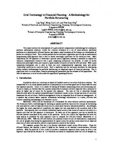
(2). If A is a Trapezoid Fuzzy Number with four elements such as: A = (T, L, M, U), then its membership function can be expressed as in Eq. (3) and Fig. 1. ( )

1 x 0

T

L

M

U

Fig.1. Trapezoid membership function

≤ ≤ ( )= ≤ ⎨ ≤ ⎪ ⎩ ≥ ⎧ ⎪

62

0 ≤ ≤ 1 ≤ 0

(4)

Journal of Optimization in Industrial Engineering 22 (2017) 61-71

2.3. Objectives description

2.3.2. Risk

The objectives for this model are defined as follows:

one of the objectives for which DM wants to attain the desired value is risk. So, we will describe as a risk:

2.3.1. Capital gain/loss

=∑

An increase/decrease in capital asset in a defined period of time. The decision-makers will try to maximize probability of the expected gaining of portfolio. It is assumed that is the expected return of portfolio, so: =∑

= 1, … ,

n

(5)

=

( ,

)⁄

(

)

(12)

Sharp risk coefficient. Capital percentage that is allocated to the stock i. The number of stocks in portfolio. The rate of return of stock i. The rate of return of market. ( )

Expected return of i th stock of portfolio. Capital percentage that is allocated to the i th stock. n the number of stocks in portfolio. is the minimum value that DM desired to attribute to , while tolerance of and is minimum probability risked for this value If we want to consider the probability that DM prefers to attain, we can formulate the objective as: (∑

≥

)≥

1

x 0

(6)

=∑

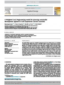
Fig. 3. fuzzy number of constraints (13)

(7)

is the minimum value that DM desired to attribute to while the tolerance of and is minimum probability risked for this value, so we attain (13):

Based on the central limit theorem, if N is sizable enough, then has normal distribution, and we attain (7): ( )

( )

(

( )

≥ )

~ (0,1)

( )+

(8)

( )≤

(13)

The fuzzy number of these objectives is depicted in Fig.3. ( ) ( ( ) ( )

)

≤

≥

( ) ( )

≥

⟷ ( )+

⟷

( )

≤

(9)

( )≥

(10)

( )

2.3.3. divided yield another objective that we will use is divided yields, a financial ratio that shows how much a company pays out in dividends each year, depending on its share price in the absence of any capital gains, while the divided yield is the return on investment for a stock, and here we show it with .

( )

=∑

(14)

1

Divided yields of stock i Capital percentage that is allocated to the stock i. x

0

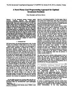
( ) Fig. 2. fuzzy number of constraints (10)

1

If we consider the minimum value that DM desires to attain, we can add fuzziness concept to our objective and rewrite (9). ( )+

( )≥

x

0

(11)

Fig. 4. fuzzy number of constraints (14)

The fuzzy number of this objective is depicted in Fig 2.

Desirable level for objective

63

is

, so:


∑

≥

objectives. According to the fuzzy decision proposed by Bellman and Zadeh (1970), all the fuzzy objectives are combined to form a fuzzy decision H which is a fuzzy set, resulting from the intersection of all the fuzzy objectives, characterized by its membership function as follows:

(15)

The fuzzy number of this objective is depicted in Fig 4 2.4. FGP Formulation

=

The multiple-objective optimization problems are often described as follows: ( ) = 1, … ,

(17)

(18)

( )≥

=

+ 1, … , .

(19)

( )=

=

+ 1, … ,

(20)

∈ ( )⊂

(21)

( )

0 1 =

( )

0

≤ ( )≤

= 1, … ,

+ 1, … ,

(22)

(23)

( )

≤ ( )≤

,..,

Considering the explanation above, we can formulate our model as below:

Where is the aspiration level of the ith objective; ( ) ≤ (≥ =) means that the ith objective is approximately less than or equal to (approximately greater than or equal to, Or approximately equal to) the aspiration level . The fuzzy objectives can be identified as fuzzy sets defined over the feasible set with the membership functions. For the above three types of fuzzy objectives, linear membership functions, according to Zimmermann (1978-1983), are defined as follows: 1 ( )≤ =

,

The above model uses the min-operator to aggregate all the fuzzy objectives to determine a decision set, and then maximizes the min-operator to simultaneously optimize all the fuzzy objectives for obtaining a higher overall satisfaction grade. However, if some particular objectives are difficult to achieve, then achievement degrees of the other objectives may decrease by this approach. Chen and Tsai (2001) illustrated this situation by an example given by Narasimhan (1980).

= 1, … ,

=

. . ℎ ≤ , = 1, … , ∈ ( )⊂

Where ''opt' 'means finding the optimal solution x which satisfies all the objectives; ( , , … , ) is decision vector, ( ) is the ith objective, and ( ) includes the constraints. In a fuzzy environment, goal programming problems can, in general, be represented by a FGP model and contain three kinds of fuzzy goals as follows:

s.t. ( ) ≤

⋀ … ⋀

Then, the resulting linear programming formulation of Eq. (20) is

(16)

. . ∈ ( ) ⊂

⋀

= , … ,

3.

A Numerical Example

In order to show the efficiency of our proposed model more clearly, we have considered a numerical example based on the data of securities on the NYSE. Four portfolios have been created that have eighteen stocks, the information of which has been summarized in Tables (1),(2),(3),(4). The last column of tables shows the average price of each stock in the last fifty days.

(24) Where (or ) is the lower (or upper) tolerance limit for the i th fuzzy objective. The membership functions can be regarded as the achievement degrees of the fuzzy

64


Table 1

Table 3 Portfolio three, having been made based on Google finance information (www.google.com/finance)

Portfolio one, having been made based on Google finance information (www.google.com/finance) Num ber

Company name

1

ARMOUR Residential REIT, Inc.

Symbol 50d avg price

Number

Company name

Symbol

50d avg price

1

Addus Homecare Corporation

ADUS

9.8

ARR

7.51

2

Adecoagro SA

AGRO

8.18

2

Alcoa Inc.

AA

8.85

3

Adept Technology Inc

ADEP

3.3

3

Belo Corp.

BLC

7.57

4

Advanced Micro Devices, Inc.

AMD

2.59

4

AEGON N.V. (ADR)

AEG

5.26

5

Actuate Corporation

BIRT

6.04

5

Gerdau SA (ADR)

GGB

9.55

6

Anthera Pharmaceuticals Inc

ANTH

0.65

6

FXCM Inc

FXCM

9.71

7

Grupo Radio Centro SAB de CV (ADR)

RC

8.23

7

Anworth Mortgage Asset Corporation

ANH

6.19

8

Cryolife Inc

CRY

5.7

8

Artio Global Investors Inc.

ART

2.51

Arts-Way Manufacturing Co. Inc. ARTW

6.66

9

KeyCorp

KEY

8.51

9

10

Roundy's Inc

RNDY

7.72

10

Asanko Gold Inc

AKG

3.34

11

Silvercorp Metals Inc. (USA)

SVM

5.92

11

BFR

4.47

12

Pengrowth Energy Corp (USA)

PGH

6.86

BBVA Banco Frances S.A. (ADR)

13

Whiting USA Trust I

WHX

8.63

12

BBX Capital Corp

BBX

7.99

14

Xerox Corporation

XRX

7.35

13

BRT Realty Trust

BRT

7.04

6.22

14

BSD Medical Corporation

BSDM

1.44

15

BSQUARE Corporation

BSQR

3.16

16

BTU International, Inc.

BTUI

2.73

17

Alpha and Omega Semiconductor Ltd

AOSL

8.2

18

Ballantyne Strong Inc

BTN

3.8

15

Box Ships Inc

TEU

16

Noranda Aluminum Holding Corporation

NOR

6.54

17

Safe Bulkers, Inc.

SB

6.08

18

CSX Corporation

CSX

7.57

Table 2 Portfolio two, having been made based on Google finance information (www.google.com/finance) Number

Company name

Symbol

50d avg price

1

1-800-FLOWERS.COM, Inc.

FLWS

4.49

2

1st Century Bancshares, Inc.

FCTY

5.26

3

1st Constitution Bancorp

FCCY

4

1st United Bancorp Inc (Florida)

5 6

Table 4 Portfolio four, having been made based on google finance information (www.google.com/finance) Number

Company name

Symbol

50d avg price

1

Ballard Power Systems Inc. (USA)

BLDP

0.89

8.92

2

Baltic Trading Ltd

BALT

3.62

FUBC

6.29

3

Banco Bilbao Vizcaya Argentaria SA (ADR)

BBVA

9.67

21Vianet Group Inc

VNET

9.57

4

Banco Santander, S.A. (ADR)

SAN

7.65

8x8, Inc.

EGHT

6.73

5

Bank of Virginia

BVA

5.47

6

Bank of the James Financial Group, Inc.

BOTJ

7.47

7

BankFinancial Corporation

BFIN

7.9

8

Banro Corporation (USA)

BAA

2.22

9

Belo Corp

BLC

9.06

10

Beneficial Intrst of Invsc Snr Incm Trst

VVR

5.56

Beneficial Mutual Bancorp Inc

BNCL

9.69

7

A. H. Belo Corporation

AHC

5.38

8

ACADIA Pharmaceuticals Inc.

ACAD

6.59

9

ACCO Brands Corporation

ACCO

7.62

10

ADDvantage Technologies Group, Inc.

AEY

11

AEterna Zentaris Inc. (USA)

AEZS

2.38

12

AMREP Corporation

AXR

9.65

11

13

ANADIGICS, Inc.

ANAD

2.24

12

Acquity Group Ltd

AQ

6.81

14

API Technologies Corp

ATNY

2.65

13

Berkshire Bancorp Inc

BERK

8.3

15

ARC Document Solutions Inc

ARC

2.56

14

Brookline Bancorp, Inc.

BRKL

9.1

15

Brooks Automation, Inc.(USA)

BRKS

9.93

16

DWS Global High Income Fund

LBF

9.02

17

Daegis Inc

DAEG

1.26

18

Danaos Corporation

DAC

3.74

2.24

16

AU Optronics Corp. (ADR)

AUO

4.17

17

AVEO Pharmaceuticals, Inc.

AVEO

7.3

18

AXT Inc

AXTI

2.92

65


The data for this section have been picked out from the Google finance, and they refer to the S&P 500 index, daily stock returns of each portfolio dating from 7 Mar 2012 to 10 Sep 2012 which has been used. DM preferences for each portfolio have been presented in Table 5. For instance, as for DM, the best preferable return for portfolio one is higher than 0.02 with membership function of one, and the worst condition is zero that has membership of zero. Preferable risk is lower than 0.5 with membership function of 1, and the unacceptable range is higher than 1.2. For divided yield, the range higher than 0.034 has membership function of 1 and lower than 0.01 with membership function of zero.

The model is solved as a non-linear goal programming by Lingo11 software and the results of which are summarized in Table 7. Table 7 shows percentage of the investment in each stock in defined portfolio considering the related scenarios, defined as well. Table 8 shows the objective and membership functions values of the defined objective. After solving model with each scenario, we can use this information in the decision process. With regard to the results, it is assumed that DM has decided to invest in portfolio one considering the scenario two, in portfolio two considering the scenario one, in portfolio three considering the scenario one, in portfolio four considering the scenario one, during a period of one month from 10 Sep 2012 to 19 Oct. Using the real data from google finance database, we calculated the real value of objectives represented in Table 9.

Table 5 DM preferences about parameters of the model Portfolio 1 objectives

Minimum

Maximum

Return

0

Upper than 0.02

Risk

Lower than 0.5

1.2

Divided yield

0.01

Upper than 0.034

We compared the presented model with Markowitz basic model; as we know, Markowitz’s mean variance approach requires minimizing the risk of the selected asset portfolio while guaranteeing a pre-established return rate as well as the total use of the available capital. If we add the objective of divided yield to the Markowitz model, we have: (Markowitz 1952):

Portfolio 2 Objectives

Minimum

Maximum

Return

-0.003

Upper than 0.01

Risk

Lower than 0.3

0.8

Divided yield

0.01

Upper than 0.02

= (∑ ) (40) = (∑ ) (41) =∑ (42) . ∶ ≤ (43) Expected return of i th stock of portfolio. Divided yields of stock i Capital percentage having been allocated to the i th stock. n the number of stocks in portfolio. Expected return for portfolio The risk of portfolio Divided yield A Constraint matrix b maximum level of constraints


Minimum

Maximum

Return

0

Upper than 0.02

Risk

Lower than 0

0.5

Divided yield

0.01

Upper than 0.03


Minimum

Maximum

Return

-0.01

Upper than 0.03

Risk

Lower than 0

0.5

Divided yield

0.01

Upper than 0.04

Five scenarios were defined for goals of risk and return; each scenario explains the probability that DM prefers to attain for each portfolio which is presented in table 6. For instance, in scenario one, DM prefers to attain a defined level with probability of fifty percent.

1

2

3

4

5

Risk

50%

40%

60%

50%

40%

Return

50%

50%

70%

40%

80%

= (

=

=

. ∶

Table 6 Scenarios for risk and return defined by DM Number

66

≤

) (

)

Table 7 Results of solving model for each portfolio considering defined scenarios scenarios Number Portfolio 1 2 3 4 5 6 7 8 9 10 11 12 13 14 15 16 17 18

1 P1 ARR 0.2 AA 0 BLC 0 AEG 0.087 GGR 0 FXCM 0 RC 0.081 CRY 0.22 KEY 0.042 RNDY 0.006 SVM 0.069 PGH 0 WHX 0.020 XRX 0.004 TEU 0.035 NOR 0 SB 0 CSX 0.1

P2 FLWS 0 FCTY 0 FCCY 0 FUBC 0 VNET 0.48 EGHT 0 AHC 0.29 ACAD 0 ACCO 0.095 AEY 0.020 AEZS 0 AXR 0 ANAD 0 ATNY 0 ARC 0 AUO 0 AVEO 0 AXTI 0.1

2 P3 ADUS 0 AGRO 0.09 ADEP 0.07 AMD 0 BIRT 0 ANTH 0 ANH 0.20 ART 0 ARTW 0 AKG 0.41 BFR 0 BBX 0 BRT 0.21 BSDM 0 BSQR 0 BTUI 0 AOSL 0 BTN 0

P4 BLDP 0 BALT 0 BBVA 0 SAN 0.090 BVA 0 BOTJ 0 BFIN 0 BAA 0.65 BLC 0 VVR 0 BNCL 0.030 AQ 0.020 BERK 0 BRKL 0.19 BRKS 0 LBF 0 DAEG 0.004 DAC 0

P1 ARR 0.32 AA 0 BLC 0 AEG 0.087 GGR 0 FXCM 0 RC 0.081 CRY 0.22 KEY 0.042 RNDY 0.006 SVM 0.069 PGH 0 WHX 0.020 XRX 0.0004 TEU 0.035 NOR 0 SB 0 CSX 0.1

P2 FLWS 0.033 FCTY 0.040 FCCY 0.028 FUBC 0.032 VNET 0.043 EGHT 0.033 AHC 0.16 ACAD 0.032 ACCO 0.091 AEY 0.064 AEZS 0.046 AXR 0.034 ANAD 0.041 ATNY 0.043 ARC 0.041 AUO 0.043 AVEO 0.043 AXTI 0.14

3 P3 ADUS 0.023 AGRO 0.1 ADEP 0.048 AMD 0.053 BIRT 0.075 ANTH 0.049 ANH 0.044 ART 0.049 ARTW 0.12 AKG 0.049 BFR 0.052 BBX 0.009 BRT 0.05 BSDM 0.05 BSQR 0.05 BTUI 0.057 AOSL 0 BTN 0.1

P4 BLDP 0.091 BALT 0.027 BBVA 0.036 SAN 0.021 BVA 0.045 BOTJ 0.069 BFIN 0.052 BAA 0.091 BLC 0.022 VVR 0.020 BNCL 0.12 AQ 0.1 BERK 0.036 BRKL 0.026 BRKS 0.025 LBF 0.022 DAEG 0.087 DAC 0.091

P1 ARR 0.2 AA 0.099 BLC 0 AEG 0.0002 GGR 0.5 FXCM 0 RC 0 CRY 0 KEY 0 RNDY 0 SVM 0.099 PGH 0 WHX 0 XRX 0 TEU 0 NOR 0 SB 0 CSX 0.1

P2 FLWS 0 FCTY 0 FCCY 0 FUBC 0 VNET 0 EGHT 0 AHC 0 ACAD 0 ACCO 0.050 AEY 0.020 AEZS 0 AXR 0 ANAD 0 ATNY 0 ARC 0 AUO 0 AVEO 0 AXTI 0.93

4 P3 ADUS 0.09 AGRO 0 ADEP 0 AMD 0.0002 BIRT 0.08 ANTH 0 ANH 0 ART 0 ARTW 0 AKG 0.0001 BFR 0 BBX 0.001 BRT 0 BSDM 0 BSQR 0 BTUI 0.0002 AOSL 0 BTN 0.82

P4 BLDP 0 BALT 0 BBVA 0 SAN 0 BVA 0 BOTJ 0 BFIN 0.34 BAA 0 BLC 0 VVR 0 BNCL 0.03 AQ 0.23 BERK 0 BRKL 0 BRKS 0 LBF 0 DAEG 0 DAC 0.28

P1 ARR 0.2 AA 0 BLC 0 AEG 0 GGR 0.6 FXCM 0 RC 0 CRY 0 KEY 0 RNDY 0 SVM 0 PGH WHX 0 XRX 0 TEU 0 NOR 0.1 SB 0 CSX 0.1

P2 FLWS 0 FCTY 0.83 FCCY 0 FUBC 0 VNET 0 EGHT 0 AHC 0 ACAD 0 ACCO 0.050 AEY 0.020 AEZS 0 AXR 0 ANAD 0 ATNY 0 ARC 0 AUO 0 AVEO 0 AXTI 0.1

5 P3 ADUS 0.85 AGRO 0 ADEP 0 AMD 0.005 BIRT 0.08 ANTH 0.006 ANH 0 ART 0 ARTW 0.008 AKG 0 BFR 0.004 BBX 0 BRT 0 BSDM 0 BSQR 0 BTUI 0.036 AOSL 0 BTN 0

P4 BLDP 0.85 BALT 0 BBVA 0.019 SAN 0.07 BVA 0 BOTJ 0.001 BFIN 0 BAA 0 BLC 0 VVR 0 BNCL 0.03 AQ 0.02 BERK 0.0003 BRKL 0 BRKS 0 LBF 0 DAEG 0 DAC 0

P1 ARR 0.34 AA 0 BLC 0 AEG 0.081 GGR 0 FXCM 0 RC 0.079 CRY 0.22 KEY 0.042 RNDY 0.0066 SVM 0.065 PGH 0 WHX 0.019 XRX 0.0034 TEU 0.034 NOR 0 SB 0 CSX 0.1

P2 FLWS 0 FCTY 0.49 FCCY 0.20 FUBC 0 VNET 0 EGHT 0 AHC 0 ACAD 0 ACCO 0.084 AEY 0.020 AEZS 0 AXR 0 ANAD 0.030 ATNY 0 ARC 0.035 AUO 0 AVEO 0 AXTI 0.13

P3 ADUS 0.09 AGRO 0 ADEP 0 AMD 0.013 BIRT 0.08 ANTH 0.001 ANH 0 ART 0 ARTW 0 AKG 0.006 BFR 0 BBX 0.084 BRT 0 BSDM 0 BSQR 0 BTUI 0.026 AOSL 0 BTN 0.69

P4 BLDP 0 BALT 0 BBVA 0 SAN 0 BVA 0 BOTJ 0 BFIN 0.17 BAA 0 BLC 0 VVR 0 BNCL 0.03 AQ 0.2 BERK 0 BRKL 0 BRKS 0 LBF 0 DAEG 0 DAC 0.77


Table 8 Value of objective function following the solving model considering the defined scenarios 1 P1 V 0 1.19 0.01

Objectives Return Risk Divided yield

P2 M 0.01 0.02 0.02

P3

V 0 0.68 0.012

M 0.34 0.34 0.34

V 0 0.5 0.02

M 0.34 0 0

V 0 0.7 0.0077

M 0.34 0.34 0

V 0 0.5 0

M 0.34 0.34 0

V 0 0.5 0.00012

M 0.34 0.34 0

V 0 0.5 0

P4 M 0 0 0

V 0 1.27 0.017

M 0 0 0

V 0 1.15 0.012

M 0 0 0

V 0 1.15 0.017

M 0 0 0

V 0 0.87 0.0091

M 0 0 0

V 0 0.87 0.0089

M 0.35 0 0.35

2 P1 V 0.016 0.63 0.017


P2 M 0.81 0.81 0.33

P3

V 0 0.91 0.0067

P4 M 0.35 0.35 0.08

3 P1

P2

V 0 1.2 0.01


M 0 0 1

P3

V 0 0.68 0

P4 M 0.35 0 0.15

4 P1 V 0.0012 1.15 0.01


P2 M 0.07 0.07 0.02

P3

V 0 0.68 0

P4 M 0.35 0.35 0

5 P1

P2

V 0 1.2 0.01


P1: Portfolio 1

M 0 0 0

P2: Portfolio 2

V 0 0.68 0

P3: Portfolio 3

P3

P4: Portfolio 4

P4

V: Value

M 0.35 0.35 0

M: Membership functions

Table 9 Real value of objectives after one month P1

P2

P3

P4

Return

Risk

Divided yield

Return

Risk

Divided yield

Return

Risk

Divided yield

Return

Risk

Divided yield

0.012

0.60

0.015

0.11

0.63

0.012

0.0063

1.35

0.019

0.007

1.08

0.014

The objectives of the model are calculated, considering the real data extracted from google finance that the values of objectives are presented in Table 10 for each portfolio. The basic difference between the first model (presented model) and the last one is the risk. In the first model, risk

has been calculated based on sharp coefficient; in the second one, we have variance of return. We used the result of the presented model and Markowitz constraints, calculated the risk and compared it with each other based on the model. The results are in Table11.

Table 10 Value of objectives after one month P1 Return

Risk

-0.025

0.0057

P2 Divided yield

Return

Risk

0.032

0.00019

0.00020

P3 Divided yield

Return

Risk

0.026

0.00056

0.000066

68

P4 Divided yield

Return

Risk

0.088

0.00038

0.00073

Divided yield 0.11


Table 11 Comparing risk measure in the presented model and Markowitz basic one P1 Base on Variance of return

Base on sharp coefficient

1

0.000074

0.60

2

0.0001

0.13

Risk Model

P2 Base on Variance of return


1

0.00015

0.63

2

0.00020

0.66

Risk Model



1

0.00026

1.35

2

0.000091

1.68

Risk Model



1

0.0015

1.08

2

0.00047

1.33

Risk Model

Model 1: Presented model 4.

Model 2: Markowitz basic model compared with Markowitz basic model. Comparing between Tables 8 and 9, we found that the results after a period of one month indicate to be close to or even better than what DM preferred; so, we can use this model as a reliable model. Comparing between Tables 9 and 10, we found that return has better value in model 1 (the presented model), and divided yield has better value in Markowitz basic model, but the results have values that are close together. The presented model measures the risk with sharp coefficient and Markowitz basic model with variance of return. These two models have been compared considering the risk in Table 11. In this paper, we discussed the fuzzy goal programming model with probabilistic constraints. It was assumed that the returns of risky assets were random variables and the level of objectives’ attainability had fuzzy concept. Also, three objectives of risk, return, and divided yields were defined considering the definition of objectives. We assumed that the two objectives of risk and return had

Discussion and Conclusion

Briefly, in this paper, firstly, the survey about past research studies in portfolio selection using goal programming model were discussed. Following that, the methodology used in the model was explained. Four experimental portfolios by the experts' opinion were selected in NYSE, and then DMs were asked about the scenarios and preferences of objectives for each portfolio. For testing the efficiency of the model, we invested using the output of the model. Finally, the presented model was compared with Markowitz basic one, and the risk measures in Markowitz basic model as well as the presented model were compared accordingly In this study, after presenting the goal programming model, four portfolios have been constructed using the experts' views in NYESE market; the presented model has been tested in one month, following which it has been

69


Dastkhan , H. Golmakani, H. & Gharneh , N. (2013). How to obtain a series of satisfying portfolios : a fuzzy portfolio management approach . Int j of industerial and systems Engineering,14,333-351. Fan, Z. P. Ma, J. A. & Zhang, Q. (2002). An approach to multiple attribute decision making based on fuzzy preference information on alternative. Fuzzy Sets and Systems,131, 101-106. Fan He, & Rong Qu. (2014). A two-stage stochastic mixedinteger program modelling and hybrid solution approach to portfolio selection problems. Information Sience. DOI: http://dx.doi.org/10.1016/j.ins.2014.08.028. Gupta, P. Inuiguchi, M. Mehlawat, M, K. & Mittal, G. (2012). Multiobjective credibilistic portfolio selection model with fuzzy chance-constraints. Information Science. 229 (2013), 1-17. Hallerbach, W. Ning, H. Soppe, A. & Spronk, J. (2004). A framework for managing a portfolio of socially responsible investments. European Journal of Operational Research, 153,517-529. Inuiguchi, M. & Tanino, T. (2000). Portfolio selection under independent possibilistic information. Fuzzy Sets and Systemsm,115,83-92. Jamalnia, A. & Soukhakian, M.A. (2009). A hybrid fuzzy goal programming approach with different goal priorities to aggregate production planning. Compute. Ind. Eng, 56, 1474–1486. Kumar, P. C. Philippatos, G. C. & Ezzell, J. R. (1978). Goal Programming and Selection of Portfolio by Dual-Purpose Funds . Journal of Finance, 33,303-310. Lee, S. M. & Chesser, D. L. (1980). Goal programming for portfolio selection . Journal of Portfolio Management, 6, 2226. Lee, S. M. & Lerro, A. J. (1973). Optimizing the portfolio selection for mutual funds. Journal of Finance, 28, 10861101. Le َ◌n, T. Liem,V. & Vercher. E. (2002). Viability of infeasible portfolio selection problems a fuzzy approach. European Journal of Operational Research,139, 178-189. Levary, R. R. & Avery, M. L. (1984). On the practical application of weighting equities in a portfolio via goal programming. Op research, 21, 246-261. Markowitz, H.H. (1952). Portfolio selection. Journal of Finance, 7, 77-91. Merton, RC. (1972). An analytic derivation of the efficient frontier. Journal of Finance and Quantitative Analysis, 7, 1851-1872. Mohiuuddin Rather, A. (2012). Portfolio selection using meanrisk model and mean risk diversification model. Int. J. of operational Research,14,324-342. Modirii, M. Moheb, S. & Heidari,H. (2010). Influence of fuzzy goal programming production optimization case study: Cement industry. Journal of optimization in industrial engineering. Number 6, 2010, 43-52. Narasimhan, R. (1980) .Goal programming in a fuzzy environment . Decis. Sci, 11,325-336. Pendaraki, K. Doumpos, M. & Zopounidis,C. (2004) . Towards a goal programming methodology for constructing equity mutual fund portfolios. Journal of Asset Management, 4, 415-428. Perold, AF. (1984). Large-scale portfolio optimization. Management Science, 3,1143-1160. Schniederjans, M. J., (1992). Allocating total wealth: A goal programming approach. Computers & Operations Research, 20, 679-685.

normal distributions, and that divided yield was discrete. We solved the model with different probabilities considering DM preference. DM accepted one of these patterns for investment. Here, probability can be described as the risk of attaining the objectives. We used the objectives of Markowitz (risk and return) and added the objective of divided yield to it, then we tried to maximize return and divided yield and minimize the risk. After one month, we measured our objectives in represented model and Markowitz’s constraint -based model, in which the basic difference between these two models was risk measure. In our model, risk measure is based on sharp coefficient; in Markowitz’s, risk is based on variance of return. We calculated the risk with two patterns of sharp coefficient and variance of return using the result of the presented model and Markowitz’s constraint-based one. The results are presented in Table 10. Obviously, the results of the presented model are better when we calculate the risk based on variance of return and coefficient measure of sharp. Also, we can see that the result of divided yield in our model is better than Markowitz’s constraint-based model; mean of return in Markowitz’s basic model is a little better than that of our model. In the presented model, we also used two definitions of risk: one is related to sharp coefficient and another to the probability of attaining the objectives of risk and return. For future studies, we recommend using stochastic programming with fuzzy concept, recognizing more objectives and presenting one decision support system (DSS) for selecting portfolio, recognizing the indices that have effect on the risk and return of portfolio, and using fuzzy logic for selecting portfolio.

References Alinezhad, A., Zohrebandian, M., Kian, M., Ekhtiari, M., & Esfandiari, N. (2011). Extension of portfolio selection problem with fuzzy goal programming: A fuzzy allocated portfolio approach. Journal of optimization in industrial engineering. Number 9, 2011, 69-76. Bellman, R.E., & Zadeh, L.A.(1970). Decision-making in a fuzzy environment. J.Manag. Sci,17,141-164. Charnes, A., & Cooper, WW. (1961). Management model and industrial application of linear programming.Wiley, Newyork,1. Chen, C. T. (2001). A fuzzy approach to select the location of the distribution center. Fuzzy Sets and Systems, 118,65-73. Chen, C.T. (2000) . Extensions of the TOPIS for group decisionmaking under fuzzy environment. Fuzzy Sets and Systems,114,1-9. Chen, L.H., & Tsai, F.C. (2001). Fuzzy goal programming with different importance and priorities .Eur. J. Oper. Res,133, 548-556. Dash, G. H. & Kajiji, N. (2002). Evolving Economy Bank Asset-Liability and Risk Management Under Uncertainty with Hierarchical Objectives and Nonlinear Pricing. Journal of Multi Criteria Decision Analysis, 11, 247-260.

70


manufacturing system. European Journal of Operational Research,154, 563-572. Watada, J. (1997). Fuzzy portfolio selection and its applications to decision making. Tatra Mountains Mathematical Publication,13, 219-248. Wu, H. Zeng, Y. & Yao, H. (2013). Multi-period Markowitz's mean–variance portfolio selection with state-dependent exit probability. Economic Modeling. 36 (2014), 69-78. Zadeh, L.A. (1965). Fuzzy Sets. Inform and Control, 8,338-353. Zhang, W.G. Xiao, W.L. (2007). On weighted lower and upper possibilistic means and variances of fuzzy numbers and its application in decision. Knowledge and Information Systems,10, 1007-10115. Zimmermann, H.J. (1983). Fuzzy mathematical programming. Fuzzy Sets Syst, 10,291-298. Zimmermann, H.J. (1978). Fuzzy programming and linear programming with several objective functions. Fuzzy Sets Syst,1, 45-56.

Sharma, J. K. Dinesh, K. & John, O. (2002). Optimal portfolio selection: A goal programming approach. Indian Journal of Finance and Research,7, 67-76. Sharpe, W. F. (1971) A linear programming approximation for the general portfolio analysis problem. Journal of Financial and Quantitative Analysis, 6, 1263–75. Sharpe, W. F. (1967) .A linear programming algorithm for mutual funds portfolio selection. Management Science, 13, 499-510. Sharpe, WF. (1970). Portfolio theory and capital markets. ( New York: McGraw-Hill). Stone, B. K. (1973). A linear programming formulation of the general portfolio selection problem. Journal of Financial and Quantitative Analysis, 8,621-636. Voros, J. (1986). Portfolio analysis-An analytic derivation of the efficient portfolio frontier. European Journal of Operational Research, 23,294-300. Wang, J. & Lin, Y. I. (2003). A fuzzy multi-criteria group decision making approach to select configuration items for software development. Fuzzy Sets and Systems,134,343-363. Wang, R. C. & Chuu, S. J. (2004). Group decision-making using a fuzzy linguistic approach for evaluating the flexibility in a

This article can be cited: Kazemi, A., Shakourloo, A. & Alinezhad, A. (2017). A Fuzzy Goal Programming Model for Efficient Portfolio Selection. Journal of Optimization in Industrial Engineering.10 (22), 61-71. URL: http://qjie.ir/article_277.html

DOI: 10.22094/joie.2017.277

71