A Fuzzy Goal Programming model for solving ...

Energy Economics 45 (2014) 196–204

Contents lists available at ScienceDirect

Energy Economics journal homepage: www.elsevier.com/locate/eneco

A Fuzzy Goal Programming model for solving aggregate production-planning problems under uncertainty: A case study in a Brazilian sugar mill Aneirson Francisco da Silva ⁎, Fernando Augusto Silva Marins Sao Paulo State University, Department of Production, Brazil

a r t i c l e

i n f o

Article history: Received 11 February 2012 Received in revised form 6 May 2014 Accepted 12 July 2014 Available online 24 July 2014 JEL classification: C61 C63 C65

a b s t r a c t This paper proposes a Fuzzy Goal Programming model (FGP) for a real aggregate production-planning problem. To do so, an application was made in a Brazilian Sugar and Ethanol Milling Company. The FGP Model depicts the comprehensive production process of sugar, ethanol, molasses and derivatives, and considers the uncertainties involved in ethanol and sugar production. Decision-makings, related to the agricultural and logistics phases, were considered on a weekly-basis planning horizon to include the whole harvesting season and the periods between harvests. The research has provided interesting results about decisions in the agricultural stages of cutting, loading and transportation to sugarcane suppliers and, especially, in milling decisions, whose choice of production process includes storage and logistics distribution. © 2014 Elsevier B.V. All rights reserved.

Keywords: Aggregate production planning Goal Programming Fuzzy Goal Programming Sugar and ethanol mills

Brazilian Sugar and Ethanol Milling Companies have recently faced a major organizational change, and industry management is changing due to the international importance of their products, especially ethanol and electricity. The evolution of the sugarcane plantation in Brazil: an increase in the 2010 harvest compared to the previous year was noted, being the Central-South region responsible for more than 80% of the Brazilian national production (Conab, National Supply Company, 2011). Unfortunately, few quantitative models and optimization methods can be applied in the planning of industrial tasks of sugar and ethanol milling companies (Paiva and Morabito, 2009). Moreover, Jamalnia and Soukhakian (2009) pointed that traditional Mathematical Programming techniques are not suitable to solve realworld aggregate production planning problems. Özcan and Toklu (2009) commented that Goal Programming (GP) is a useful branch of the Multiple Criteria Decision-Making (MCDM), perhaps, the oldest and the most widely used MCDM technique to solve

multi-objective problems. Caballero et al. (2009) also commented that GP has been successfully applied in many different areas. As discussed by Wang and Liang (2004) real-world problems related to aggregate production planning are usually ill-defined, with more than one (and, eventually, conflicting) important objective. Besides, decisionmakers are not generally able to specify precise goal values (baselines) to the objectives to be optimized, to the coefficients in the objective functions and to the constraints. The same is occurring with righthand side coefficients associated with available resource quantities. In fact, according to Chang (2007), imprecise aspiration levels (goals, baselines) may exist to the enterprise objectives, a typical situation in the sugarcane agro-industry where many uncertainties, such as: commodity markets, raw material quality, and results of production processes are inherent to their planning process. Thus, all these indicate that GP and Fuzzy Logic are very interesting decision tools to be used to solve this kind of problems. Next, we present a few characteristics of this research that differ from those found in specialized literature on aggregate productionplanning under uncertainty:

⁎ Corresponding author at: Sao Paulo State University, Av. Ariberto Pereira da Cunha, 333, CEP 12.516-410 Guaratingueta, SP, Brazil. Tel.: +55 12 3123 2866. E-mail addresses: [email protected] (A.F. da Silva), [email protected] (F.A.S. Marins).

– Development of a Fuzzy Goal Programming model for the aggregate production problem under uncertainty in a sugar mill company; – Integration of the agricultural, industrial, and logistics phases into a unique model, to support decision-makings during harvest seasons and periods between harvests.

1. Introduction

http://dx.doi.org/10.1016/j.eneco.2014.07.005 0140-9883/© 2014 Elsevier B.V. All rights reserved.

A.F. da Silva, F.A.S. Marins / Energy Economics 45 (2014) 196–204

197

This paper is organized into Sections. In Section 2 we present the GP and Fuzzy Logic concepts. In Section 3 we present the adopted research method. Section 4 refers to the description of the aggregate production-planning problem and its FGP model. Section 5 summarizes the model optimization, and, finally, the conclusions and suggestions for future researches are in the Section 6, followed by the references. 2. Fuzzy Goal Programming One of the benefits of using multi-objective optimization models is the possibility of extracting a set of meaningful information related to the analyzed problem, enabling different analysis (Bellman and Zadeh, 1970; Chang, 2007; Deb, 2001). Zimmermann (1978) was the first to solve a Linear Programming problem with several objectives through a fuzzy programming approach that used the concept of the membership function introduced by Zadeh (1965). The Fuzzy Set (FS) theory, proposed by Zadeh (1965), is based on the extension of the classical definition of set A, where each element x of a given universe X, either belongs to set A or not, whereas in the FS theory an element belongs to set A with a certain “degree of membership”. In classic models of GP, the decision maker has to specify a precise aspiration level (goal) for each of the objectives. In general, especially in large-scale problems, this is a very difficult task, and the use of the Fuzzy Set theory in GP models can overcome such problem, allowing decision makers to work with imprecise aspiration levels (Yaghoobi and Tamiz, 2007). Therefore, an objective with an imprecise aspiration level can be regarded as a fuzzy goal. There are three most common types of fuzzy goals to work with triangular fuzzy numbers (Jamalnia and Soukhakian, 2009; Yaghoobi and Tamiz, 2007). These types are given by expressions (1)–(3), where the symbol ~ is a fuzzifier that represents the imprecise fashion in which the goals are stated, and gk is the aspiration level for kth goal: e k; k ¼ 1; …; m Gk ðxÞ ≤g

e k. Fig. 2. Gk ðxÞ ≥g

of tolerance limits is very important as they directly influence the performance of the model optimization. Fuzzy goals can be identified as fuzzy sets defined over the feasible set with a membership function. Linear membership functions are the most adopted functions, both in theoretical and in practical works (Jamalnia and Soukhakian, 2009). For the above three types of fuzzy goals here are the following linear membership functions: 8 1 > > > > U k −Gk ðxÞ < μ Zk ðxÞ ¼ U k −g k > > > > : 0

ð2Þ

Gk ðxÞ≅g k ; k ¼ n þ 1; …; l

ð3Þ

A fuzzy goal can be identified as the fuzzy sets defined over the feasible set with the membership function. The three fuzzy goals above are illustrated from Figs. 1 to 3, where Lk (Uk) is the lower (upper) limit for the kth fuzzy goal Gk(x). Usually, limits Lk and Uk are either subjectively chosen by decision makers or associated with tolerances in a technical process. The choice

e k. Fig. 1. Gk ðxÞ ≤g

if g k ≤Gk ðxÞ≤U k if Gk ðxÞ ≥U k

; k ¼ 1; …; m ð4Þ

8 1 > > > G ðxÞ−L > < k k μ Zk ðxÞ ¼ g k −Lk > > > > : 0

if Gk ðxÞ≥g k if Lk ≤Gk ðxÞ≤g k if Gk ðxÞ≤Lk

; k ¼ m þ 1; …; n ð5Þ

ð1Þ

e k ; k ¼ m þ 1; …; n Gk ðxÞ ≥g

if Gk ðxÞ ≤g k

μ Zk ðxÞ ¼

8 0 > > > G ðxÞ−L > > k k > > > g −L < k

k

> > U k −Gk ðxÞ > > > > U −g > > k k : 0

if Gk ðxÞ≤Lk if Lk ≤Gk ðxÞ≤g k ; k ¼ n þ 1; …; l

ð6Þ

if g k ≤Gk ðxÞ≤U k if Gk ðxÞ≥U k

According to Chang (2007), since Narasimhan (1980) has applied the FS set theory with a preference-based membership function to GP, many achievements have been made in areas related to Fuzzy Goal Programming (FGP), including preemptive, weight additive, and stochastic models. As proposed by Yaghoobi and Tamiz (2007), a FGP model based

Fig. 3. Gk(x) ≅ gk.

198


on the MINMAX approach (due to Flavell, 1976), can be expressed by: Max μ

ð7Þ

S. t: þ

f i ðxÞ−di ≤bi ; −

f i ðxÞ þ di ≥bi ; −

þ

i ¼ 1; 2; …; i0

i ¼ i0 þ 1; …; j0

f i ðxÞ þ di −di ¼ bi ;

i ¼ j0 þ 1; …; K

ð8Þ

ð9Þ ð10Þ

μþ

1 − d ≤ 1; ΔiR i

i ¼ 1; …; i0

ð11Þ

μþ

1 þ d ≤1; ΔiL i

i ¼ i0 þ 1; …; J 0

ð12Þ

μþ

1 − 1 þ d þ d ≤1; ΔiL i ΔiR i

þ

−

μ; di ; di ≥0;

X∈F

i ¼ j0 þ 1; …; K

ð13Þ

i ¼ 1; …; K

ð14Þ

F is a feasible set

ð15Þ

where, in the notation proposed by Yaghoobi and Tamiz (2007), bi is the aspiration level for the ith goal, ΔiR and ΔiL indicates, respectively, the admissible violations to the right and left for the ith fuzzy goal; Cs is an + optional set of rigid (inviolable) constraints, d− i and di are the negative and positive deviation variables for the ith goal, fi(X) is the objective functions and μ is a degree achievement fuzzy function with 0 ≤ μ ≤ 1, standardized and dimensionless, is associated with each objective function.

3. Research method The research phases illustrated in Fig. 4 are explained in the sequence: – Problem identification — Milling companies were visited and one was chosen to be the object of study (case). A revision of the technical literature was also made focusing on the production of sugar, alcohol, molasses and sub-products, in order to understand the elements and set the scope of the problem (see Section 4); – Data collection — Data were collected internally, and members of staff (managers and engineers) were interviewed in order to double check the quality of the available information. Some of these data are not presented here due to confidential information; – Modeling — The multi-objective mathematical modeling was developed for the case, incorporating the harvest season and periods between harvests, accounting for 52 weeks of milling activities (see Section 4); – Experiment — The data collected in (b) were used to model the problem with the software GAMS — General Algebraic Modeling System, version 24.2.1, while the Solver CPLEX 12.6 was used in order to find an optimum solution for the model (see Section 5); – Validation — Performed with the support of technical professionals (specialists) of the studied company. The specialists analyzed the results of the model solution and compared them with the real results for the last harvest, in order to check coherence and applicability of the model results; – Implementation — This phase depends on the company's decision, but it is important to emphasize that the research was considered adequate in all its technical aspects. 4. Problem description and its modeling 4.1. Problem description Here we present the main characteristics of the aggregate planning problem, including logistics decisions, in a typical Brazilian Sugar and Ethanol Milling Company (BSEMC). The first step to understand the problem was mapping the industrial process. The industrial process involves the subdivisions of the sugarcane juice flow, the use of molasses, the type of ethanol and sugar being

Fig. 4. Research steps.


199

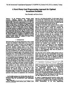
Fig. 5. Sugar, ethanol and molasses process flow (source: Paiva and Morabito, 2009).

produced, the sugarhouse recovery efficiency, the efficiency of the distillery, and the overall sucrose waste, as illustrated in Fig. 5. Fig. 5 illustrates the nine most important unitary operations related to the milling processes (weighing, warehouse, wash, mill, clarification), to sugar and molasses production (evaporation, crystallization) and to ethanol distillery (fermentation, distillation). Fig. 5 also depicts the waste of sucrose in every step of the industrial process (washing, milling, clarification, undetermined, fermentation, and distillation losses). For more details, please consult Paiva and Morabito (2009). A Fuzzy Goal Programming (FGP) model was developed to solve the multi-objective aggregate production-planning problem under uncertainty for a BSEMC. The products are sugars – Crystal, VHP, and VVHP –, and ethanol, and the co-product is molasses. The company's manager suggested nine objectives to be achieved: – Minimize the costs of each agro-industrial phase: – Supply of raw material (sugar cane); – Sugar cane transportation; – Production process. – Minimize the total inventory cost; – Minimize the total distribution cost of the products (sugars and ethanol) to clients; – Maximize the production of Crystal sugar; – Maximize the production of VHP sugar; – Maximize the production of VVHP sugar; – Maximize the production of ethanol. 4.2. Problem modeling The FGP model for the aggregate production-planning problem in the sugar mill (FGP-APPSM) is formulated in the sequence, and uses two matrices to prepare the input data before its optimization:

- Matrix of Industrial Processes (MIP) composed by the quantity of each product p (sugars — Crystal, VHP, and VVHP, and ethanol) produced by each process k (weighing, warehouse, wash, mill, clarification, evaporation, crystallization, fermentation, and distillation) for a given period t (harvest and between harvest or 52 weeks);

– Matrix of Industrial Costs (MIC) composed by the cost of using each process k in each period t; Sets k t p p1 p2 p3 p4 m f e i l π

industrial processes, k ∈ K, K = {1,2,…,24}; planning periods, t ∈ T, T = {1,2,…,52}; final products, p ∈ P, P = {VHP, VVHP, Crystal, ethanol}; production of the VHP sugar; production of the VVHP sugar; production of the Crystal sugar; production of ethanol; sugarcane suppliers, m ∈ M, M = {owned and rented}; sugarcane transport providers, f ∈ F, F = {owned and rented}; inventory positions, e ∈ E, E = {number of warehouses of the company and rented places – own and rented}; Clients, i ∈ I, I = {1,2,…,30}; distributors of sugars and ethanol, l ∈ L, L = {owned and rented}; values of goals for the nine objectives chosen by the BSEMC, π ∈ Π, Π = {1,2,…,9}.

Parameters Mtmin minimum milling capacity [ton/week]; Mtmax maximum milling capacity [ton/week]; CTf capacity of the transport provider f [ton/week]; αt maximum percentage of farmers' sugarcane in period t [%]; βf t availability of transport provider f in period t [%]; φt percentage of available operation time in the plant in period t [%]; γt forecasted efficiency of milling shutdowns in period t [%]; Cestp e inventory capacity of product p in each position of storage e [ton or m3]; L1f t variable cost of cutting, loading and transporting sugarcane with the transport provider f in period t [$/ton]; hp e variable cost of inventory of product p in each position of storage e [$/ton or $/m3]; hsp e cost of inventory in the after harvesting period of product p in each position of storage e [$/ton or $/m3]; DSp t demand of product p in period t [ton or m3]; Vp t revenue of product p in period t [$/ton or $/m3];

200


Ip e 0 Dispm 0 M'm 0 MIPp

k t

MICk t MACm t

CACp

i l t

initial inventory of product p in each position of storage e [ton or m3] before starting the planning period; sugarcane harvesting forecast of the sugarcane supplier m [ton] before starting the planning period; quantity of sugarcane harvested by the supplier m [ton] before starting the planning period; Element of the Matrix of Industrial Processes (MIP) — representing the quantity of product p made on each industrial process k in period t [ton or m3]; Element of the Matrix of Industrial Costs (MIC) — representing the cost of the industrial process k in period t [$/ton]; Element of the Matrix of Agricultural Costs (MAC) — representing the cost associated to the sugarcane supplier m in period t [$/ton]; shipping cost of product p to client i using the transport provider l in period t [$].

Fig. 7. Membership function of Z2.

Goal Z3: Maximize the total VHP sugar production [ton]:

Decision variables

X XX

xkt

p1 ∈P k∈K t∈T

mt mmt′ m″ft m‴kt xapilt dispmt Ipet

decision variable associated to the selection of the process k in period t (xkt = 1 or =0); quantity of sugarcane crushed in period t [ton]; quantity of sugarcane sent from the sugarcane supplier m in period t [ton]; quantity of sugarcane transported by the transport provider f in period t [ton]; quantity of sugarcane crushed by process k in period t [ton]; quantity of product p to be delivered to client i using transport provider l in period t [ton or m3]; availability of sugarcane in the supplier m in period t [ton]; inventory of product p in each position of storage e in period t [ton or m3].

Auxiliary variables d+ variable of deviation of over-achievement for each fuzzy goal; π d− variable of deviation of under-achievement for each fuzzy π goal; μπ achievement degree for each fuzzy goal, and that, 0 ≤ μ ≤ 1. In the sequence, we introduce the fuzzy concepts to obtain the FGP model. Please note that BSEMC specialists estimated the goal values (right-hand side values):

p3 ∈P k∈K t∈T

‴

mk t :MIP p3 kt ¼27; e 500

ð16Þ

p2 ∈P k∈K t∈T

Goal Z4: Maximize the total ethanol production [m3] X XX

‴

mk t :MIP p4kt ¼86; e 000

ð19Þ

p4 ∈P k∈K t∈T

Goal Z5: Minimize the total storage costs [$]: X XX

e 000 Ip e t :hp e t ≤950;

ð20Þ

p∈P e∈E t∈T

Goal Z6: Minimize the total raw-material transport costs from the sugarcane suppliers [$]: XX

″ e 676; 000 m f t :L1 f t ≤26;

ð21Þ

f ∈ F t∈T

Goal Z7: Minimize the total raw-material costs from the sugarcane suppliers [$]: X X

0 e 400; 000 mmt :MACm t ≤51;

ð22Þ

m∈M t∈T

XX

‴

e 500; 000 mk t :MIC k t ≤9;

ð23Þ

k∈K t∈T

Goal Z9: Minimize the total distribution costs to the clients [$]:

Goal Z2: Maximize the total VVHP sugar production [ton]: X XX

ð18Þ

Goal Z8: Minimize the total raw-material processing costs [$]:

Goal Z1: Maximize the total Crystal sugar production [ton]: X XX

‴

mk t :MIP p1kt ¼15; e 500

‴

mk t :MIP p2 kt ¼30; e 500


ð17Þ

XXXX

e 700; 000 xap i l t :CAC p i l t ≤1;

p∈P i∈I l∈L t∈T


ð24Þ


201

Fig. 11. Membership function of Z6. Fig. 9. Membership function of Z4.

The maximum and minimum limits for the deviations of each fuzzy goal are illustrated in Figs. 6 to 14, and for more details see Figs. 1 to 3. – Eq. (25) is the fuzzy achievement (objective) function: Max Z ¼

X

μk

X ð25Þ

π∈Π

– Eq. (26) is the small bucket constraint in each period t: X

xk t ¼ 1;

∀t∈T

planted is not available for the present season, this amount is not taken into consideration by the model:

ð26Þ

dispmt ¼

m∈M

– Inequality (33) is the capacity constraint for the quantity of sugarcane crushed in each period t: min

X

I pet ¼ I 0 þ

X

e∈E

I p e t−1 þ

e∈E

X

mt :MIP pkt −DAC p t −xap i l t

∀p∈P; ∀t∈T

k∈K

ð27Þ

Mt

:

ϕt γ t γ max ϕ : ≤mt ≤M t : t : t 100 100 100 100

X

0

mmt ¼

″ mft

f∈F

X

m f t″ ;

∀t∈T

ð28Þ

f∈F

m∈M

X

X

¼

X

mmt ≤α t :mt

∀∈T

ð29Þ

ð33Þ

∀m∈M; ∀t∈T

ð34Þ

– Inequality (35) is the constraint over the quantity of sugarcane transported by the mill owned transport system f in period t: ″

‴ mkt ;

∀t∈T

– Inequality (34) restricts the amount of sugarcane supplied by farmers and by the mill owners (rent and owned, respectively) that is going to be crushed in period t: 0

– Eqs. (28)–(30) are the compatibility constraints (one stage model).

ð32Þ

mt

t∈T

k∈K

– Eq. (27) is the inventory balancing of final product p, for client i in period t:

X

mft ≤

β f t γt : : CT f 100 100

∀f ∈F; ∀t∈T

ð35Þ

k∈K

‴

mkt ¼ mt ;

∀∈T

ð30Þ

k∈K

– Constraint (36) imposes that the quantity of sugarcane processed by process k in period t (m‴kt) should be zero if process k is not used (in this case xkt = 0), and it should be less than or equal to Mmax , t otherwise xkt = 1: ‴

– Eq. (31) is the sugarcane m availability constraint in each period t: 0

dispmt ¼ dispmt−1 −mmt−1

∀m∈M; ∀t∈T

ð31Þ

– Eq. (32) is the constraint of utilization of the sugarcane available in the harvesting season. It is assumed that if part of the sugarcane


max

mkt ≤M t

xk t

∀k∈K; ∀t∈T

ð36Þ

– Inequality (37) is the constraint over inventory capacity of product p in each position of storage e in period t: Ipet ≤Cest pe

∀p∈P; ∀e∈E; ∀t∈T


ð37Þ

202


– Eqs. (46)–(47) are associated with the total VHP sugar production: X XX

‴

−

þ

mkt :MIP p1kt þ d5 −d5 ¼ 15; 000

ð46Þ

p1 ∈P k∈K t∈T

μ5 þ

1 1 þ − :d þ :d ≤1 15; 000−13; 000 5 17; 000−15; 000 5

– Eqs. (48)–(49) are associated with the total VVHP sugar production:


X XX − Fuzzy Goal Constraints: d+ π and dπ are positive and negative deviation variables for the ith fuzzy goal. – Equations (38–39) are associated with the total storage costs:

X XX

þ

I p e t :hp e t −d1 ≤976; 000

ð38Þ

p∈P e∈E t∈T

ð39Þ

μ6 þ

XX

″

þ

mft :L1ft −d2 ≤26; 676; 000

ð40Þ

f ∈ F t∈T

μ2 þ

1 þ :d ≤1 26; 800; 000−26; 600; 000 2

ð41Þ

– Eqs. (42)–(43) are associated with the total raw-material costs from suppliers: XX

0

þ

mmt :MACmt −d3 ≤51; 400; 000

ð42Þ

m∈M t∈T

μ3 þ

þ

ð48Þ

1 1 þ − :d þ :d ≤1 31; 000−29; 000 6 33; 000−31; 000 6

ð49Þ

‴

−

þ

mkt :MIP p3kt þ d7 −d7 ¼ 26; 000

ð50Þ

1 1 þ − :d þ d ≤1 26; 000−23; 000 7 29; 000−26; 000 7

ð51Þ

p3 ∈P k∈K t∈T

– Eqs. (52)–(53) are associated with the total ethanol production: X XX p4 ∈P k∈K t∈T

μ8 þ

‴

−

þ

mkt :MIP p4 k t þ d8 −d8 ¼ 85; 000

ð52Þ

1 1 þ − :d þ :d ≤1 86; 000−84; 000 8 88; 000−86; 000 8

ð53Þ

– Eqs. (54)–(55) are associated with the total raw-material processing costs: XXXX

þ

xap i l t :CAC p i l t −d9 ≤1; 700; 000

ð54Þ

p∈P i∈I l∈L t∈T

1 þ :d ≤1 51; 600; 000−51; 400; 000 3

ð43Þ

– Eqs. (44)–(45) are associated with the total raw-material processing costs: XX

−

– Eqs. (50)–(51) are associated with the total Crystal sugar production:

μ7 þ – Eqs. (40)–(41) are associated with the total raw-material transport cost from suppliers:

‴

mkt :MIP p2kt þ d6 −d6 ¼ 30; 000

p2 ∈P k∈K t∈T

X XX 1 þ :d ≤1 μ1 þ 950; 000−900; 000 1

ð47Þ

‴

þ

mkt :MIC kt −d4 ≤9; 540; 000

ð44Þ

1 þ :d ≤1 9; 700; 000−9; 500; 000 4

ð45Þ

μ9 þ

1 þ :d ≤1 1; 700; 000−1; 500; 000 9

ð55Þ

– Expression (56) represents the integrality and non-negativity

k∈K t∈T

μ4 þ


Table 1 Comparison between the Brazilian Sugar and Ethanol Milling Company (BSEMC) planning for 2010/2011 season and the results obtained from the FGP-APPSM model. Results

(a) FGP-APPSM

(b) BSEMC

Difference

Production of Crystal sugar [ton] Production of VHP sugar [ton] Production of VVHP sugar [ton] Total production of sugars [ton] Production of AEHC [m3] Total ART [kg/ton] Total sugarcane ART [kg/ton] Final industrial efficiency [%] Revenue [$]

26,956

24,400

10.48%

14,500

13,780

5.22%

31,854

29,820

6.82%

73,310

68,000

7.81%

85,800 207.30 223.8 90.8 ($) 33,305,891.36

84,360 207.17 223.7 90.3 ($) 31,196,975.80

1.71% 0.063% 0.045% 0.55% 6.76%

A.F. da Silva, F.A.S. Marins / Energy Economics 45 (2014) 196–204 Table 2 Results for the fuzzy goals. Goal π

μ

Maximize production of Crystal sugar [ton] Maximize production of VHP sugar [ton] Maximize production of VVHP sugar [ton] Maximize production of AEHC [m3] Minimize the total ART [kg/ton] Minimize the total storage costs Minimize the total raw-material transport costs from sugarcane suppliers Minimize the total raw-material processing costs Minimize the total distribution costs to clients

1 1 0.8 1 1 1 1 1 1

constraints: 0

″

‴

xk t ∈f0; 1g; mt ≥ 0; mmt ≥ mft ≥ 0; mkt ≥0; dispmt ≥0; I p e t ≥0; xap i l t ≥ 0;

þ − dπ ; dπ ≥ 0; ∀p∈P; ∀e∈E; ∀k∈K; ∀m∈M; ∀t∈T; ∀f ∈F; ∀i∈I; ∀l∈L; ∀π∈Π

ð56Þ

203

from the 2010/2011 seasons with excellent results, according to BSEMC managers. After the model optimization only the fuzzy goal associated with the production of the VVHP sugar was not fully satisfied, presenting a value of 0.8; the other fuzzy goals had values equal to 1, in other words, the other fuzzy goals were fully satisfied, as shown Table 2. The final validation of the FGP-APPSM model was made with the support of the BSEMC administrative manager. He compared the results of the model with the plant's actual results for the 2010/2011 season, and concluded that the proposed model can be applied to the aggregate production-planning problem, once it has established feasible and consistent production plans for all the analyzed periods. A fact praised by the manager was that the model development allowed a better understanding of the decision variables and the parameters involved, and promoted a greater interaction between professionals of the BSEMC consulted about the agricultural, industrial and logistics phases related to the aggregate production-planning problem under uncertainty. 6. Conclusions and future research directions

5. Results of the FGP model application in a real case The BSEMC — Brazilian Sugar and Ethanol Milling Company, situated in the Southeast region of Brazil, is able to produce various types of sugar: VHP, VVHP, Crystal; one of the main types of fuel: hydrated ethanol (AEHC); a sugarhouse co-product: molasses; besides some sub-products such as filter mud, bagasse, vinasse and fusel oil. In a typical harvesting season, the BSEMC crushes 1.8 million tons of sugarcane and produces 150,000 tons of sugar and 1,000,000 m3 of ethanol. The present case study was carried out using data from the 2010/2011 harvesting and between harvest seasons, and the aim was to analyze if the proposed FGP-APPSM model could improve the corresponding aggregate production planning. The model resulted in 5530 variables, where 1248 were binary, 9682 constraints, and 41,233 nonzero elements. For the real application of the FGP-APPSM model, an Intel (Core i7) 1.26 GHz processor, with 8 GB RAM and operational system from Microsoft 64 bits was used, and the model was solved using the modeling language GAMS 24.2.1 with the optimization solver CPLEX 12.6. The total elapsed real time was 2.2 h. Some of the results are in Table 1. In analyzing Table 1, we can observe that the model results recommend a higher production of ethanol than sugar; and that the VVHP sugar has preference over Crystal and VHP sugar. Another observation in Table 1 concerns the overall industrial efficiency: both plans involved almost the same values (see difference of 0.55%), which means that technically the model solution is close to the reality of the FGP-APPSM. However, the most important result in Table 1 is the total value of the variable revenue. In analyzing such important aspect we conclude that the total variable revenue associated with the FGP-APPSM model is 6.76% higher than the result obtained by the planning of the FGPAPPSM for the same season. These results encourage the use of the FGP-APPSM model to support decisions in the aggregate production planning and in the logistics of Sugar and Ethanol Milling Companies. Managers could adopt a rolling strategy, for the planning horizon, to solve the FGP-APPSM model, considering all weeks of the harvesting season, and then, as soon as each subsequent week data are available, do a data upgrading and solve the model one more time for the remaining weeks until the end of the season. With this strategy, the aggregate production-planning problem and its analysis become a routine and the impact of data uncertainty is minimized. This strategy was applied in the FGP-APPSM using data

This paper presents a Fuzzy Goal Programming (FGP) model to support decisions in the aggregate production-planning under uncertainty in sugar and ethanol milling companies. The FGP model provides useful information for decision makers, helping them to better understand the variables and the important issues involved in the problem. In fact, the proposed model provides an effective analysis of these issues, offering more reliable and more precise outputs, from technical and economical perspectives. Other advantages of the FGP-APPSM model are: – It facilitates the analysis of different scenarios in decision-making processes, replacing subjective, incomplete, and under uncertainty judgments; – It supports managers in the analysis of the results obtained in the aggregate production-planning and how to work with unexpected situations; – It encourages an integration of decisions in the agricultural, and industrial stage, and in the logistics distribution of final products to meet marketing requirements. It is worth saying that sucroenergetic industries have similar processes, this way, the FGP model proposed here may be easily used in other plants. However, so that this model can be applied in other sucroenergetic industries, managers shall balance goals, that is, the pertinent uncertainties to each fuzzy goal, once these goals depend on weather conditions and on sugarcane varieties, which may be different in each region of the country, as well as, on the company's production and sales strategy. The results of this study are promising and encouraged us to continue this research. Nowadays, we are developing new models that: – Incorporate the production of energy using sugarcane bagasse; – Allow the analysis of the application of the Response Surface Methodology (MONTGOMERY, 2005) to the design of the raw material mixture in industrial processes in order to improve yields and costs;

Acknowledgments This research was partially supported by The National Council for Scientific and Technological Development (CNPq -303362/2012-0 and 470189/2012), and by The Coordination for the Improvement of Higher Education Personnel (CAPES - PE- 024/2008), and São Paulo Research Foundation (FAPESP - 2014/06374-2).

204


Appendix A. Supplementary data Supplementary data to this article can be found online at http://dx. doi.org/10.1016/j.eneco.2014.07.005. References Bellman, R.E., Zadeh, L.A., 1970. Decision making in a fuzzy environment. Manag. Sci. 17, 141–164. Caballero, R., Gomez, T., Ruíz, F., 2009. Goal programming: realistic targets for the near future. J. Multi-Criteria Decis. Anal. 16 (3–4), 79–110. Chang, C.-T., 2007. Multi-choice goal programming. Int. J. Manag. Sci. 35, 389–396. Conab (National Supply Company), 2011. Technical report. Available at: http://www. conab.gov.br/conabweb/download/safra/1cana_de_acucar.pdf (Acessed on august 23). Deb, K., 2001. Multi-objective Optimization using Evolutionary Algorithms. John Wiley and Sons, England. Flavell, R.B., 1976. A new goal programming formulation. Omega. Int. J. Manag. Sci. 4, 731–732.

Jamalnia, A.,Soukhakian, M.A., 2009. A hybrid fuzzy goal programming approach with different goal priorities to aggregate production planning. Comput. Ind. Eng. 56, 1474–1486. Montgomery, D., 2005. Design and Analysis of Experiments, 6th edition. John Wiley & Sons, Inc. Narasimhan, R., 1980. Goal programming in a fuzzy environment. Decis. Sci. 11, 325–336. Özcan, U., Toklu, B., 2009. Multiple-criteria decision-making in two-sided assembly line balancing: a goal programming and a fuzzy goal programming models. Comput. Oper. Res. 36, 1955–1965. Paiva, R.P.O., Morabito, R., 2009. An optimization model for the aggregate production planning of a Brazilian sugar and ethanol milling company. Ann. Oper. Res. 169, 117–130. Wang, R.C., Liang, T.F., 2004. Application of fuzzy multi-objective linear programming to aggregate production planning. Comput. Ind. Eng. 46, 17–41. Yaghoobi, M.A.,Tamiz, M., 2007. A method for solving fuzzy goal programming problems based on MINMAX approach. Eur. J. Oper. Res. 177, 1580–1590. Zadeh, L.A., 1965. Fuzzy sets. Inf. Control. 8, 338–353. Zimmermann, H.-J., 1978. Fuzzy programming and linear programming with several objective function. Fuzzy sets and systems functions. Fuzzy Sets Syst. 1, 45–55.