A Fuzzy Logic Based Set of Measures for Software Project Similarity: Validation and Possible Improvements Ali Idri and Alain Abran Software Engineering Management Research Laboratory Department of Computer Science UQAM, P.O Box. 8888,. Centre-Ville Postal Station Montréal, Québec, Canada, H3C 3P8
[email protected] [email protected] Abstract The software project similarity attribute has not yet been the subject of in-depth study, even though it is often used when estimating software development effort by analogy. Among the inadequacies identified (Shepperd et al.) in most of the proposed measures for the software project similarity attribute, the most critical is that they are used only when the software projects are described by numerical variables (interval, ratio or absolute scale). However, in practice, many factors which describe software projects, such as the experience of programmers and the complexity of modules, are measured in terms of an ordinal (or nominal) scale composed of qualifications such as ‘very low’, ‘low’ and ‘high’. To overcome this limitation, we propose a set of new measures for similarity when the software projects are described by categorical data. These measures are based on fuzzy logic: the categorical data are represented by fuzzy sets and the process of computing the various measures uses fuzzy reasoning. In this work, the proposed measures are validated by means of an axiomatic validation approach, using a set of axioms representing our intuition about the similarity attribute and verifying whether or not each measure contradicts any of the axioms. We also present in this paper the results of an empirical validation of our similarity measures, based on the COCOMO’81 database.
1. Introduction The similarity of two software projects, which are described and characterized by a set of attributes, is often evaluated by measuring the distance between these two projects through their sets of attributes. Thus, two projects are not considered similar if the differences between their sets of attributes are obvious. It is important to note that the similarity of two software projects also depends on
their environment: projects which are similar in a specific type of environment may not necessarily be similar in other environments. So, according to Fenton’s definitions [5], similarity will be considered as an external product attribute and, consequently, one which can only be measured indirectly. The way in which the similarity of software projects is gauged is fundamental to the estimation of software development effort by analogy, and a variety of approaches have been proposed in the literature [12]. Shepperd et al. [13,14] found three major inadequacies while investigating similarity measures. The first of these is that they are computationally intensive, and, consequently, many Case-Based Reasoning systems have been developed, such as ESTOR[15] and ANGEL[13]. The second is that the algorithms are intolerant of noise and of irrelevant features. The third and most critical is that they cannot handle categorical data other than binaryvalued variables. However, in software metrics, specifically in software cost estimation models, many factors (linguistic variables in fuzzy logic), such as the experience of programmers and the complexity of modules, are measured on an ordinal scale composed of qualifications such as ‘very low’ and ‘low’ (linguistic values in fuzzy logic). For example, in the COCOMO’81 model, 15 attributes out of 17 (22 out of 24 in the COCOMO II model) are measured with six linguistic values: ‘very low’, ‘low’, ‘nominal’, ‘high’, ‘very high’ and ‘extra-high’ [2,3,4]. Another example is the Function Points measurement method, in which the level of complexity for each item (input, output, inquiry, logical file or interface) is assigned using three qualifications (‘low’, ‘average’ and ‘high’). Then there are the General System Characteristics, the calculation of which is based on 14 attributes measured on an ordinal scale of six linguistic values (from ‘irrelevant’ to ‘essential’) [8]. To overcome this problem, we are proposing a set of similarity measures which are based on fuzzy logic and which can therefore be used when software projects are
unsharp boundaries. It is considered as an extension of classical set theory. The membership function µA(x) of x in a classical set A, as a subset of the universe X, is defined by: 1 iff x ∈ A µ A ( x ) = 0 iff x ∉ A
described by categorical variables [7]. Such proposed measures must, of course, be validated. Consequently, in this work we present the results of an axiomatic validation approach for our measures, as well as the results of an initial empirical validation. This empirical validation is based on the COCOMO’81 database. This paper is organized as follows: In the first section, we briefly outline the principles of fuzzy logic and we stress what we called the normal condition. In the second section, we present a set of candidate measures for similarity when software projects are described by categorical variables. In the third section, we validate the measures by using an axiomatic validation approach. The axiomatic validation of measures is the process whereby we ensure that the measures do not contradict any intuitive notions about the similarity of two software projects. Our intuition will be codified by a set of axioms. In the fourth section, the similarity measures, which were declared valid in the previous section, will be empirically validated; many remarks and observations will be made on the basis of this empirical validation. Consequently, in the fifth section, we present suggestions for improving our similarity measures. A conclusion and an overview of future work conclude this paper.
This means that an element x is either a member of set A (µA(x)=1) or not (µA(x)=0). Classical sets are also referred to as crisp sets. For many classifications, however, it is not quite clear whether x belongs to a set A or not. For example, in [10], if set A represents PCs which are too expensive for a student’s budget, then it is obvious that this set has no clear boundary. Of course, it could be said that a PC priced at $2500 is too expensive, but what about a PC priced at $2495 or $2502? Are these PCs too expensive? Clearly, a boundary could be determined above which a PC is too expensive for the average student, say $2500, and a boundary below which a PC is certainly not too expensive, say $1000. Between those two boundaries, however, there remains an interval in which it is not clear whether a PC is too expensive or not. In this interval, a grade could be assigned to classify the price as partly too expensive. This is where fuzzy sets come in: sets in which the membership has grades in the interval (0,1). The higher the membership x has in fuzzy set A, the more true it is that x is A. The fuzzy set, introduced by Zadeh, is a set with graded membership in the real interval (0,1). It is denoted by:
2. Fuzzy logic Since its foundation by Zadeh in 1965 [20], Fuzzy Logic (FL) has been the subject of important investigations. At the beginning of the nineties, fuzzy logic was firmly grounded in terms of its theoretical foundations and its application in the various fields in which it was being used (robotics, medicine, image processing, etc.). The aim in this section is not to discuss fuzzy logic in depth, but rather to present those parts of the subject that are necessary for an understanding of this paper. According to Zadeh [22], the term “fuzzy logic” is currently used in two different senses. In a narrow sense, FL is a logical system aimed at a formalization of approximate reasoning. In a broad sense, FL is almost synonymous with fuzzy set theory. Fuzzy set theory, as its name suggests, is basically a theory of classes with
∫
A = µ A ( x) / x X
where µA(x) is known as the membership function and X is known as the universe of discourse. Figure 1 shows two representations of the linguistic value ‘too expensive’; the first using a fuzzy set (Figure 1 (a)) and the second using a classical set (Figure 1 (b)). The major advantage of the fuzzy set representation is that it is a gradual function rather than an abrupt-step function between the two boundaries of $1000 and $2500.
µ too exp ensive ( x)
µ too exp ensive ( x)
1
1
0
1000
2500
$
0
1000 (a) Figure 1. Fuzzy set (a) and Classical set (b) for the linguistic value ‘too expensive
2500 (b)
$
2.1 Operations on fuzzy sets As for classical sets, operations are defined on fuzzy sets, such as intersection, union, complement, etc. In the literature on fuzzy sets, a large number of possible definitions are proposed to implement intersection, union and complement. For example, general forms of intersection and union are represented by triangular norms (T-norms) and triangular conorms (T-conorms or S-norms) respectively. A T-norm is a two-place function from [0,1]×[0,1] to [0,1] satisfying the following criteria [10]: T-1 T(a, 1) = a T-2 T(a, b) ≤ T(c, d), whenever a≤c, b≤d T-3 T(a, b) = T(b, a) T-4 T(T(a, b),c) = T(a, T(b, c)) The condition defining a T-conorm (S-norm), besides T-2, T3 and T-4, is: S-1 S(a, 0) = a Table 1 gives examples of the operators used most often. T-norm
µA∩B = min (µA(x), µB(x)) µA∩B = µA(x) ×µB(x) µA∩B = max (µA(x)+µB(x)-1, 0)
S-norm
µA∪B = max (µA(x),µB(x)) µA∪B = min (µA(x)+µB(x)-1, 0)
Table 1. Examples of T-norm and S-norm operators
2.2 Properties of fuzzy sets In the following, we present three commonly used fuzzy set properties [10]: Property 1: Fuzzy set A is called normal if the height of A, hgt(A), is equal to 1. hgt ( A) = sup µ A ( x) x∈ X
Property 2: Fuzzy set A is called convex if it is characterized by: ∀ x1 , x 2 , x 3 ∈ X
x1 ≤ x 2 ≤ x3
µ A ( x 2 ) ≥ min( µ A ( x1 ), µ A ( x 3 ))
Property 3: A tuple of fuzzy sets (A1, A2, .., AM) is called a fuzzy partition of universe X if: ∀x ∈ X ,
M
∑ µ A ( x) = 1 j =1
j
A tuple of fuzzy sets (A1, A2, .., AM) satisfy the normal condition if (A1, A2, .., AM) is a fuzzy partition and each Ai is normal and convex Among the other branches of fuzzy set theory are fuzzy arithmetic, fuzzy graph theory and fuzzy data analysis.
3. Similarity measures based on fuzzy logic The goal is to measure the similarity of two software projects P1 and P2 when their attributes are described by categorical values (linguistic values in fuzzy logic). In the software measurement literature, these categorical data are represented by classical intervals (or step functions). So, no project can occupy more than one interval. This is a serious problem in that it can lead to a great difference in effort estimations in the case of similar projects with a small incremental size difference, since each would be placed in a different interval of a step function [6]. Consequently, we have used fuzzy sets with a membership function rather than classical intervals to represent the categorical data. The advantages of this representation are as follows: § It is more general; § It mimics the way in which humans interpret linguistic values; § The transition for one linguistic value to a contiguous linguistic value is gradual rather than abrupt. Using such a representation, new similarity measures have been proposed [7]. Let projects P1 and P2 be described by M linguistic variables (Vj), and, for each linguistic variable Vj, a measure with linguistic values is defined ( Akj ). Each linguistic value, Akj , is represented by a fuzzy set with a membership function ( µ Akj ). Our measures of the similarity of P1 and P2 operate on two levels: § Measurement of similarity of P1 and P2 according to only one dimension at a time (one variable Vj), d v ( P1 , P2 ) . j
§ Measurement of similarity of P1 and P2 according to all dimensions (all variables Vj), d(P1, P2). Figure 2 summarizes the process for computing the various measures.
3.1 First step: Project similarity according to one dimension, d v (P1 , P2 ) j
A j ≠ Φ and
Aj ≠ X
An important condition, which it is often satisfied in practice, arises if a fuzzy partition (A1, A2, .., AM) is formed by normal and convex fuzzy sets. In the rest of this paper, such a condition will be called a normal condition (NC):
The first step consists in calculating the similarity of P1 and P2 according to each individual attribute with a linguistic variable Vj, d v ( P1, P2 ) . Since each Vj is j
measured by fuzzy sets, the distance d v ( P1, P2 ) must j
expresses the fuzzy equality according to Vj of P1 and P2.
RBASE
d v ( P1 , P2 ) 1
RBASE_V1
Aggregation MIN MAX I − OR
d v ( P1 , P2 ) 2
RBASE_V2
Aggregation
P1
d(P1, P2)
P2
d v ( P1 , P2 ) M
RBASE_VM
Aggregation
Figure 2. The computing process for the various measures, d v (P1 , P2 ) and d(P1, P2) j
This fuzzy set must have a membership function with two variables (Vj(P1) and Vj(P2)). This type of fuzzy set is referred to in fuzzy set theory as a fuzzy relation. Such a fuzzy relation can represent an association or a correlation between elements of the product space. In our case, the association that will be represented by this fuzzy relation is the statement P1 and P2 are approximately equal according to Vj. We denote this fuzzy relation by R≈v . j
v
is a combination of a set of fuzzy relations R≈v, k . Each
v
the equality of Vj according to one of its
R≈ j
j
R≈,jk represents
linguistic values Akj . Indeed, R≈v, k represents the fuzzy ifj
then rule, where the premise and the consequence consist of fuzzy propositions: vj ≈, k
R
j k
j k
: if V j ( P1 ) is A then V j ( P2 ) is A
Hence, for each variable Vj, we have a rule base (RBASE_Vj) which contains the same number of fuzzy ifthen rules as the number of fuzzy sets defined for Vj. Each RBASE_Vj expresses the fuzzy equality of two software projects according to Vj, dv ( P1, P2 ) . When we consider all
this is done is different for the various types of fuzzy implication functions adopted for the fuzzy rules. These fuzzy implication functions are based on distinguishing between two basic types of implication: the fuzzy implication which complies with the classical conjunction and the fuzzy implication which complies with the classical implication [10]. Using this basic distinction of two types of fuzzy implication, we have obtained three formulas for dv ( P1, P2 ) : j
max min( µ A j ( P1 ), µ A j ( P2 )) k k k max − min aggregation ∑ µ Akj ( P1 ), µ Akj ( P2 ) d v j ( P1, P2 ) = k sum − product aggregation max(1 − µ A j ( P1 ), µ A j ( P2 )) min k k k min − Kleene − Dienes aggregation dv j ( P1, P2 )
(1.1)
(1.2)
(1.3)
equal to 1 implies a perfect similarity between
P1 and P2 according to Vj; equal to 0, a total absence of similarity; between 0 and 1, a partial similarity.
j
variables Vj, we obtain a rule base (RBASE) which contains all rules associated with all variables. RBASE expresses the fuzzy equality of two software projects according to all variables Vj, d(P1, P2). dv ( P1, P2 ) is j
defined by combining all fuzzy rules in DBASE_Vj to obtain one fuzzy relation ( R≈v ) which represents j
DBASE_Vj. This combining of fuzzy if-then rules R≈v, k j
vj
into a fuzzy relation R≈ is called aggregation. The way
3.2 Second step: Project similarity according to all dimensions, d(P1, P2) We calculate the distance d(P1, P2) from the various distances dv ( P1, P2 ) : j
d ( P1 , P2 ) = F (d v ( P1 , P2 ),..., d v ( P1 , P2 )) 1
M
where M is the number of variables describing the projects P1 and P2, and F can be any function with M variables from [0,1]M to IR+. Because the various
dv j ( P1, P2 )
are membership functions associated with fuzzy v R≈ j
, we have defined F as one of the three relations operators: min as a T-norm, max as an S-norm and the ior operator as a hybrid between a T-norm and an S-norm. Since in our case, the formula given in [1] can generate undefined values, we have adopted a modification in order to avoid this. Also, the modification will allow the ior operator to work as a very conservative T-norm. The three formulas obtained are: (d v j ( P1, P2 )) min j d ( P1, P2 ) = max(d v j ( P1, P2 )) j i − or (d v ( P1, P2 )) j j
2.1 2.2 2.3
where 0 ∃k , h / d vk ( P1, P2 ) = 0 and d vh ( P1, P2 ) = 1 M d v j ( P1, P2 ) i − or (d v j ( P1 , P2 )) = j =1 j otherwise M M − d P P + d P P ( 1 ( , )) ( , ) vj 1 2 vj 1 2 j =1 j =1
∏
∏
∏
We note that d(P1, P2) using these three formulas is always in the unit interval. The natural interpretation of these three formulas will be discussed in section 5.
4. Axiomatic validation of the similarity measures The software engineering community has always been aware of the need for validation. As new measures are proposed, it is appropriate to ask whether or not they capture the attribute they claim to describe. This allows us to choose the best measures from a very large number of software measures for a given attribute. However, validation of software measures is one of the most misunderstood procedures in the software measurement area. The first question is: What is a valid measure? A number of authors in software metrics have attempted to answer this question [5, 9, 11, 23, 24]. However, the validation problem has up to now been tackled from different points of view (mathematical, empirical, etc.) and by interpreting the expression ”metrics validation” differently; as suggested by Kitchenham et al: ‘What has been missing so far is a proper discussion of relationships among the different approaches’ [11]. Beyond this interesting issue, we use Fenton’s definitions to validate the two measures, dv ( P1, P2 ) and d(P1, P2) [8]: j
Validating a software measure is the process of ensuring that the measure is a proper numerical characterization of the claimed attribute by showing that the representation condition is satisfied. This is validation in the narrow sense, meaning it is internally valid; if the measure is a component of a valid
prediction system, the measure is valid in the wide sense. In this section, we deal with the validation of d v ( P1 , P2 ) j
and d(P1, P2) in the narrow sense. dv ( P1, P2 ) and d(P1, P2) satisfy the representation j
condition if they do not contradict any intuitive notions about the similarity of P1 and P2. Our initial understanding of the similarity of projects will be codified by a set of axioms. This axiom-based approach is common in many sciences. For example, mathematicians learned about the world by defining axioms for a geometry. Then, by combining axioms and using their results to support or refute their observations, they expanded their understanding and the set of rules that governs the behavior of objects. Below, we present a set of axioms that represents our intuition about the similarity attribute between software projects and we check whether or not the two measures, dv ( P1, P2 ) and d(P1, P2), satisfy these j
axioms.
4.1 Axiom 0 (specific to d v ( P, Pi ) ) j
The similarity of two projects, according to a variable Vj, is not null if these two projects have a degree of membership different from 0 to at least one same fuzzy set of Vj d v (P,Pi ) ≠ 0 iff ∃ Ak / µ A (P) ≠ 0 and µ A (Pi ) ≠ 0 j k
j
j k
To illustrate this axiom, we use the following figure:
Fuzzy Sets for Vj
1
Vj
P
1 Interval 1
(0,1) Interval 2
0 Interval 3
Figure 3. An explanatory example of Axiom 0
d v j ( P, Pi )
§ dv ( P, Pi ) must be equal to 1 if Vj(Pi) is in Interval 1; j
m(P, Pi)≤ m(P, P)
§ dv ( P, Pi ) must decrease strictly from 1 to 0 if Vj(Pi) is in j
Interval 2; § dv ( P, Pi ) must be equal to 0 if Vj(Pi) is in Interval 3. j
It is easy to show that similarity according to Vj measured by max-min or sum-product aggregations (formulas (1.1) and (1.2)) respects Axiom 0. This is not the case when it is measured by min-Kleene-Dienes aggregation (formula (1.3)). Intuitively, P and P4 are not similar according to Vj (Figure 4). So, dv ( P, P4 ) must be j
equal to 0; but by applying the formula (1.3), dv ( P, P4 ) is
4.3.1 d v (P, Pi ) using max-min aggregation. We show j
that, for any project Pi, dv ( P, Pi ) ≤ dv ( P, P ) (Appendix 1, j
j
show by a counter-example that dv ( P, Pi ) does not respect j
Axiom 2: § For Pi, µ A ( Pi ) is equal to 1 and for all other Akj (k≠k0), j k0
j
equal to 0.5!
j
Proof 1). 4.3.2 d v (P, Pi ) using sum-product aggregation. We
µ A j ( Pi ) k
is null.
§ For P, µ A ( P ) is equal to 0,7, µ A ( P ) is equal to 0.3, j k0
Fuzzy Sets for Vj
j k1
and, for all other
Akj
(k≠k0 and k≠k1), µ A (P ) is null. j k
In this case, dv ( P, Pi ) is equal to 0.7, while dv ( P, P ) is j
j
1
equal to 0.58 (0,58=0.72 + 0,32). 4.3.3 d v (P, Pi ) using min-Kleene-Dienes aggregation.
0.5
In general, dv ( P, Pi ) does not respect Axiom 2 (Figure 5).
j
j
But, if ( A1j , A2j …, Akj , …, ANj ) satisfy the normal j
P
P4
Figure 4. A counter-example showing that min-KleeneDienes aggregation does not respect Axiom 0
condition, then min-Kleene-Dienes aggregation respects Axiom 2 (Appendix 1, Proof 2). The normal condition involves that ( A1j , A2j …, Akj , …, ANj ) does not contain j
more than two overlapping fuzzy sets.
4.2 Axiom 1 Fuzzy Sets for Vj We expect any measure m of the similarity of two projects to be positive: m(P1, P2)≥0; m(P, P)>0 dv j ( P1, P2 ) ,
in all cases formulas (1.1), (1.2) and (1.3), is
always higher than or equal to 0. So, it is also the case that d(P1, P2). dv ( P, P) , when using min-Kleene-Dienes
dv j ( P, P1 ) = 0.7 dv j ( P, P ) = 0.5
0.8 0.7 0.5
j
aggregation, is higher than 0. But when it uses max-min or sum–product aggregations, it can be equal to 0. This is the case when µ A (P) is equal to 0 for all Akj . This implies
0.3 P1
j k
that project P does not have any qualification for the variable Vj. This case can be avoided if the fuzzy sets ( A1j , A2j …, Akj , …, ANj ) form a fuzzy partition for Vj. j
This is always the case in practice. Consequently dv ( P, P) j
will be considered higher than 0 for all types of aggregation.
4.3 Axiom 2
P
Figure 5: A counter-example showing that d v (P, Pi ) using j
min-Kleene-Dienes aggregation does not respect Axiom 2 4.3.4 Distance d(P, Pi). It is calculated from the distances dv ( P, Pi ) by using the min, the max or the i-or operators. j
Thus, to check whether or not d(P, Pi) respects Axiom 2, we will use the results of the validation of the distance d v ( P, Pi ) . It is easy to show that d(P, Pi) respects Axiom 2, j
The degree of similarity of any project to P must be lower than the degree of similarity of P to itself:
some is the operator used, when d v ( P, Pi ) uses max-min j
aggregation (Appendix 1, Proof 3). We proceed in the
same way to validate the distance d(P, Pi) when d v ( P, Pi ) uses sum-product or min- Kleene-dienes j
aggregation. Table 2 shows the results obtained.
d v (P, Pi ) j
d v (P, Pi ) /d(P, Pi)
d(P, Pi) Max
Min
j
i-or
Yes Yes Yes Max-min No No No Sum-product Yes if NC Yes if NC Yes if NC KleeneDienes Table 2: Results of the validation of the distance d(P,Pi) for Axiom 2
4.4 Axiom 3 We expect any measure m of the similarity of two projects to be commutative: m(P1, P2)= m(P2, P1) d v j ( P, Pi )
respects Axiom 3 when it uses max-min or
sum-product aggregation. Consequently, d(P1,P2) is also some is the operator used. But, this is not the case when d v ( P1 , P2 ) uses min-Kleene-Dienes aggregation. We can j
check that
d v j ( P, P1 )
is equal to 0.7 and d v ( P1 , P) is equal to j
0.5 (Figure 5). By looking at the results of this validation, which takes into account four axioms (Table 3 ), we can conclude that d v ( P, Pi ) using max-min aggregation respects all the j
axioms (as, consequently, does d(P,Pi)). So, according to Fenton [8], this is a valid similarity measure in the narrow sense. d v ( P, Pi ) , using sum-product aggregation does not j
respect Axiom 2. Although Axiom 2 is interesting, will retain sum-product aggregation in order to validated in the wide sense. There are three reasons this: § The difference between d v ( P, Pi ) and d v ( P, P) is j
j
we be for not
obvious if the fuzzy sets associated with Vj satisfy the normal condition. We can show that this difference, in the case where d v ( P, Pi ) is higher than d v ( P, P) , is j
similarity of two software projects according to a fuzzy variable. Consequently, any similarity measure must satisfy this axiom.
j
in the interval [-1/8, 0]. § Sum-product aggregation respects the other axioms, specifically Axiom 0. § As was noted by Zuse [24], validation in the narrow sense, contrary to validation in the wide sense, is not yet widely accepted and mostly neglected in practice. d v ( P, Pi ) , using min-Kleene-Dienes aggregation does
max-min sum-product Kleene-Dienes Yes/ Yes/ No/ Axion0 Yes/Yes Yes/Yes Axiom1 Yes/Yes No/No Yes /Yes if NC Axiom2 Yes/Yes Yes/Yes No/No Axiom3 Yes/Yes Table 3: Results of the validation of the distance d v (P, Pi ) and d(P, Pi) j
5. Towards an empirical validation of the proposed similarity measures After validation in the narrow sense of the similarity measures (the measures are measuring what they claim to measure), we present, in this section, the first results of an incomplete empirical validation (validation in the wide sense) of our measures. According to Fenton [8], a measure is valid in the wide sense if it is both valid in the narrow sense and a component of a valid prediction system. The prediction system that we consider here is the estimation of software development effort by analogy. It is based on three steps. First, each project must be described by a set of linguistic variables which must be relevant, independent, operational and comprehensive. Second, we must determine the similarity between the candidate project and each project in the historical database by using the measures that are declared valid in the narrow sense. Third, we use the known effort values from the historical projects to derive an estimate for the new project. Below, we present only the results of the two first steps. The intermediate COCOMO’81 database was chosen as the basis for this empirical validation. The original intermediate COCOMO’81 database contains 63 projects. Each project is described by 17 attributes: the software size is measured in KDSI (Kilo Delivered Source Instructions), the project mode is defined as either organic, semi-detached or embedded, and the remaining 15 cost drivers are generally related to the software environment. Each cost driver is measured using a rating scale of six linguistic values: ‘very low’, ‘low’, ‘nominal’, ‘high’, ‘very high’ and ‘extra high’. The assignment of linguistic values to the cost drivers (or project attributes) uses conventional quantification where the values are intervals (see [3], pp. 119). For example, the DATA cost driver is measured by the following ratio:
j
not respect Axiom 0 and Axiom 3. Although it respects Axiom 1 and Axiom 2, we rejected it because of Axiom 0. For us, Axiom 0 represents the definition of the
D Database size in bytes or characters = P Program size in DSI
descriptions are insufficient. So, we consider the 12 cost drivers that we have fuzzified [6]. Because the original COCOMO’81 database contains only the effort multipliers, our evaluation of the similarity will be made on an artificial dataset deduced from the original COCOMO’81 database. This artificial dataset contains 63 projects with the real values that are necessary to determine µ A (P) of the formulas (1.1) and
Then, a linguistic value is assigned to the DATA, according to the following table: Low
Nominal
High
Very High
D/P x
M
j =1
M
j
+1≥
d v j ( P, Pi )
∏ (1 − dv ( P, P)) j
j =1
M
∏ d v ( P, P) j =1
k +1
k
max(min(x, z ), min( y, w)) − xz − yw = max( x, w) − xz − wy if x < z
∏ (1 − dv ( P, Pi )) ≥ ∏ (1 − dv ( P, P)) j
k +1
k
j
j =1
using sum-product aggregation is lower than
+ 1 ⇒ d ( P, Pi ) ≤ d ( P, P )
By studying these three functions, we can note that each of them has a minimum equal to –1/8 or a maximum equal to 1/8.
j
d v j ( P, Pi ) ≤ d v j ( P, P )
Second, d(Pm, Pn) combines dv ( Pm , Pn ) by the min j
⇒ min(d v j ( P, Pi )) ≤ min(d v j ( P, P )) ⇒ d ( P, Pi ) ≤ d ( P, P)
operator. d(Pm, Pn) with
d v j ( P, Pi ) ≤ d v j ( P, P )
aggregation is denoted by d(Pm, Pn)max-min and d(Pm, Pn) with dv ( Pm , Pn ) using sum-product aggregation is denoted
j
j
⇒ max(d v j ( P, Pi )) ≤ max(d v j ( P, P )) ⇒ d ( P, Pi ) ≤ d ( P, P) j
j
Proof 4: Difference between d(Pm, Pn) using max-min aggregation and d(Pm, Pn) using sum-product aggregation We want to prove that the absolute value of the difference between d(Pm, Pn) using formula (2.1) with dv ( Pm , Pn ) which uses max-min aggregation and d(Pm, Pn) j
using the formula (2.1) with dv ( Pm , Pn ) which uses sumj
product aggregation is lower than 1/8. In the case of d(Pm, Pn) using formula (2.2), the proof is the same. We suppose that all variables satisfy the normal condition.
dv j ( Pm , Pn )
using max-min
j
by d(Pm, Pn)sum-product: ∃i0 /
d ( Pm , Pn ) max − min = d vMM ( Pm , Pn ) = min(d vMM ( Pm , Pn )) i j
∃j0 /
d ( Pm , Pn ) sum − product = d vSP ( Pm , Pn ) = j
0
j
0
min (d vSPj ( Pm , Pn )) j
= min(d vMM ( Pm , Pn ) ± ε j ) ε j ≤ j j
if i0 ≠ j0 ⇒ d vSP ( Pm , Pn ) ≤ d vSP ( Pm , Pn ) j i 0
0
⇒ d vMM ( Pm , Pn ) ± ε j0 ≤ d vMM ( Pm , Pn ) ± ε i0 j i 0
0
while d vMM ( Pm , Pn ) ≥ d vMM ( Pm , Pn ) j i 0
⇒
0
d vSPj ( Pm , Pn ) − d vMM ( Pm , Pn ) ≤ i 0
0
1 8
1 8