IEEE TRANSACTIONS ON SIGNAL PROCESSING, VOL. 54, NO. 2, FEBRUARY 2006
405
A Game Theory Approach to Constrained Minimax State Estimation Dan Simon, Senior Member, IEEE
Abstract—This paper presents a game theory approach to the constrained state estimation of linear discrete time dynamic systems. In the application of state estimators, there is often known model or signal information that is either ignored or dealt with heuristically. For example, constraints on the state values (which may be based on physical considerations) are often neglected because they do not easily fit into the structure of the state estimator. This paper develops a method for incorporating state equality constraints into a minimax state estimator. The algorithm is demonstrated on a simple vehicle tracking simulation. Index Terms—Game theory, straints, state estimation.
filter, minimax filter, state con-
I. INTRODUCTION
I
N THE application of state estimators, there is often known model or signal information that is either ignored or dealt with heuristically [11]. This paper presents a way to generalize a minimax state estimator in such a way that known relations among the state variables (i.e., state constraints) are satisfied by the state estimate. Constrained state estimation has not, to our knowledge, been studied from a game theory or minimax point of view. estimation) Interest in minimax estimation (also called began in 1981 [31], when it was noted that in dealing with noise with unknown statistics, the noise could be modeled as a deterministic signal. This replaces the Kalman filtering method of modeling the noise as a random process. This results in estimators that are more robust to unmodeled noise and uncertainty, as will be illustrated in Section V. Although state constraints have not yet been incorporated into minimax filters, they have been incorporated into Kalman filters using a variety of different approaches. Sometimes state constaints are enforced heuristically in Kalman filters [11]. Some researchers have treated state constraints by reducing the system model parameterization [27], but this approach is not always desirable or even possible [28]. Other researchers treat state constraints as perfect measurements [7], [16]. This results in a singular covariance matrix but does not present any theoretical problems [4]. In fact, Kalman’s original paper [10] presents an example that uses perfect measurements (i.e., no measurement noise). But there are several considerations that indicate against
Manuscript received July 9, 2004; revised April 4, 2005. The associate editor coordinating the review of this manuscript and approving it for publication was Dr. Dominic K. C. Ho. The author is with the Department of Electrical and Computer Engineering, Cleveland State University, Cleveland, OH 44115 USA (e-mail:
[email protected]). Digital Object Identifier 10.1109/TSP.2005.861732
the use of perfect measurements in a Kalman filter implementation. Although the Kalman filter does not formally require a nonsingular covariance matrix, in practice a singular covariance increases the possibility of numerical problems [12, p. 249], [24, p. 365]. Also, the incorporation of state constraints as perfect measurements increases the dimension of the problem, which in turn increases the size of the matrix that needs to be inverted in the Kalman gain computation. These issues are addressed in [19], which develops a constrained Kalman filter by projecting the standard Kalman filter estimate onto the constraint surface. Numerous efforts have been pursued to incorporate concontrol problems. For instance, control straints into can be achieved subject to constraints on the system time response [8], [17], [18], state variables [14], controller poles [25], state integrals [13], and control variables [1], [33]. Fewer attempts have been made to incorporate constraints filtering problems. One example is filter design into with poles that are constrained to a specific region [15]. Finite and infinite impulse response filters can be designed such that norm of the error transfer function is minimized while the constraining the filter output to lie within a prescribed envelope [26], [32]. However, to our knowledge, there have not been any filtering efforts to incorporate state equality constraints into problems. This paper generalizes the results of [30] so that minimax state estimation can be performed while satisfying equality constraints on the state estimate. The major contribution of this paper is the development of a minimax state estimator for linear systems that enforces equality constraints on the state estimate. We formulate the problem as a particular game which state estimation was shown in [30] to be equivalent to an problem. We then derive the estimator gain and adversary gain that yields a saddle point for the constrained estimation problem. filters can be impleConstrained estimators other than mented on constrained problems. The most notable alternative filtering is constrained Kalman filtering [19]. to constrained The choice of whether to use a constrained Kalman or confilter is problem dependent, but the general advanstrained estimation can be summarized as follows [6]. tages of filtering provides a rigorous method for dealing with 1) systems that have model uncertainty. filtering provides a natural way to 2) Continuous time limit the frequency response of the estimator. (Although this paper deals strictly with discrete time filtering, the methods herein can also be used to extend existing confiltering results to constrained filtering. tinuous time This is an area for further research.)
1053-587X/$20.00 © 2006 IEEE
406
IEEE TRANSACTIONS ON SIGNAL PROCESSING, VOL. 54, NO. 2, FEBRUARY 2006
3)
filtering can be used to guarantee stability margins or minimize worst case estimation error. filtering may more appropriate for systems where the 4) model changes unpredictably, and model identification and gain scheduling are too complex or time consuming. Section II of this paper formulates the problem, and Section III develops the solution through a series of preliminary lemmas and the main saddle point theorem of this paper. As expected, it turns out that the unconstrained minimax estimator is a special case of the constrained minimax estimator. Section IV discusses how the methods of this paper can be extended to inequality constraints. Section V presents some simulation results, and Section VI offers some concluding remarks. Some lemma proofs are presented in the Appendix.
error using both the bias and some other measure (e.g., mean square error or worst case error). In general, unbiased estimators are preferred over biased estimators because of their greater mathematical tractability. Lemma 1: If we have an estimator gain of the form (5) is any dimensionally appropriate matrix, then the where state estimate (4) satisfies the state constraint (2). Proof: See the Appendix. The noise in (1) is introduced by an adversary that has the goal of maximizing the estimation error. Similar to [30], we will assume that our adversary’s input to the system is given by (6)
II. PROBLEM STATEMENT
is a gain to be determined, is a given matrix, and is a noise sequence. We will assume that , are mutually uncorrelated unity-variance white noise and sequences that are uncorrelated with . This form of the adversary’s input is not intuitive because it uses the state estimation error, but this form is taken because the solution of the resulting problem results in a state estimator that bounds the infinity norm of the transfer function from the random noise terms to the state estimation error [30]. [This is discussed further following (15).] can be considered by the designer as a tuning parameter or weighting matrix that can be adjusted on the basis of our a priori knowledge about the adversary’s noise input. Suppose, for example, that we know ahead of time that the first component of the adversary’s noise input to the system is twice the magnitude of the second component, the third component is zero, etc.; then . that information can be reflected in the designer’s choice of We do not need to make any assumptions about the form of (e.g., it does not need to be positive definite or square). approaches the zero matrix, From (6), we can see that as the adversary’s input becomes purely a random process without any deterministic component. This causes the optimal minimax filter to approach the Kalman filter; that is, we obtain better root mean square (rms) error performance but not as good worst case becomes large, the minimax filter error performance. As places more emphasis on minimizing the estimation error due to the deterministic component of the adversary’s input. That is, the minimax filter assumes less about the adversary’s input, and we obtain better worst case error performance but worse rms error performance. Lemma 2: In order for the noise-free system (1) to satisfy must satisfy the the state constraint (2), the adversary gain following equality: where
Consider the discrete linear time-invariant system given by
(1) where is the time index, is the state vector, is the meaand are white noise sequences, and surement, is a noise sequence generated by an adversary. We assume that and are mutually uncorrelated unity-variance white noise sequences. In general, , and can be time-varying matrices, but we will omit the time subscript on these matrices for ease of notation. In addition to the state equation, we know (on the basis of physical considerations or other a priori information) that the states satisfy the following constraint: (2) We assume that the matrix is full rank and normalized so . In general, is an matrix, where is that . the number of constraints, is the number of states, and If , then (2) completely defines , which makes the es, which is the case in this timation problem trivial. For paper, there are fewer constraints than states, which makes the is full rank estimation problem nontrivial. Assuming that is the same as the assumption made in the constrained Kalman filtering problem [19]. We define the following matrix for notational convenience: (3) We will assume that both the noisy system and the noise-free system satisfy the above state constraint. The problem is of given the measurements to find an estimate . The estimate should satisfy the state constraint. We will restrict the state estimator to have an observer structure so that it results in an unbiased estimate [2]
(7) One way to satisfy this equality is for
to be of the form (8)
(4) The main advantage of unbiased estimators over biased estimators is that unbiased estimators make it easier to quantify the estimation error. With biased estimators, we must quantify the
is any dimensionally appropriate matrix. where Proof: See the Appendix. The estimation error is defined as follows: (9)
SIMON: GAME THEORY APPROACH TO CONSTRAINED MINIMAX STATE ESTIMATION
It can be shown from the preceding equations that the dynamic system describing the evolution of the estimation error is given as follows:
407
Define the following matrix difference equation:
(18)
(10) Since , we see that . But we also know by following a procedure similar to the proof of Lemma . Therefore, we can subtract the zero term 1 that from the error (10) to obtain the following:
Then we have the following lemma. Lemma 3: The cost function (15) is given as follows: trace
(19)
Also, the minimization of with respect to results in an estimator with the following bound for the square of the induced norm of the system: (20)
(11) However, this is an inappropriate term for a minimax problem because the adversary can arbitrarily increase by arbitrarily increasing . To prevent this, we decompose as follows: (12) where
and
evolve as follows:
(13)
Note that the induced norm reduces to the system norm when the system is time invariant. Proof: The proof follows in a straightforward way similar to Lemma 1 in [30]. The above lemma justifies the use of the term “minimax” for the state estimator. Regardless of the disturbances that enter the and , the gain from system via the noise sequences the noise to the weighted estimation error will always be less than the bound given in the above lemma. and as the nonsingular solutions to the Now define following set of equations:
(14) Motivated by [30], we define the objective function as
(21) (15)
where is any positive definite weighting matrix. The differential game is for the filter designer to find a gain sequence that minimizes , and for the adversary to find a gain sequence that maximizes . As such, is considered a funcand , which we denote in shorthand notation tion of as and . This objective function is not intuitive but is used here because the solution of the problem results in a state estimator that bounds the infinity norm of the transfer function from the random noise terms to the state estimation error [30]. This is expressed more completely in the next section in Lemma 3. III. PROBLEM SOLUTION
Nonsingular solutions to these equations are not always guaranteed to exist, in which case a solution to the minimax state estimation problem may not exist. However, if solutions to these can be computed as equations do exist, then we see that (22) so that we have explicit formulas to iteratively compute and . Also note that we have to assume that and are nonsingular. This assumption will be necessary for the proof of Lemma 4. We propose the following gain matrices for our estimator and adversary:
(23)
The solution is obtained by finding optimal gain sequences and that satisfy the following saddle point:
To solve this problem, we will write the cost function (15) in a more convenient form. Define the matrix as follows:
Note that and satisfy the gain forms in (5) and (8), which guarantees that the state estimate and the noise-free system satisfy the constraint (2). the matrix of (17) when the Lemma 4: Denote by and gains from (23) are substituted for and . Then we obtain the following for :
(17)
(24)
(16)
408
IEEE TRANSACTIONS ON SIGNAL PROCESSING, VOL. 54, NO. 2, FEBRUARY 2006
Proof: The proof closely follows that of [30, Lemma A.1] and is also available in [23]. and from (23) for Lemma 5: If in (18) we substitute and , then we obtain the given by (21). That is, . Proof: The proof closely follows the Proof of Lemma A.2 in [30] and is also available at [23]. and as follows: Now we define the matrices
gives the adversary more latitude in choosing a disturlarger bance. This makes it less likely that the designer can minimize the cost function. The mean square estimation error with the optimal gain cannot be specified because it depends on the adversary’s input . However, we can state an upper bound for the mean square estimation error as follows. Lemma 10: If the estimator gain defined by (23), then the mean square estimation error is bounded as follows:
(25)
(31)
Then we obtain the following result. satisfies the following difference equation: Lemma 6: (26) Proof: The proof closely follows that of [30, Lemma A.3] and is also available in [23]. satisfies the Lemma 7: Suppose some matrix sequence equation
This provides additional motivation for using the game theory approach presented in this paper. The estimator not only bounds the worst case estimation error but also bounds the mean square estimation error. Proof: The proof closely follows a proof presented in [30]. Now consider the special case that there are no state conmatrix equal to a zero straints. Then in (2) we can set the vector equal to a zero column vector. In row vector and the and we obtain from (21) and (23) the folthis case, lowing estimator and adversary strategies:
(27) . Then for all . Similarly, if the matrix where sequence satisfies the above difference equation with the initial and , then for all . condition Proof: The proof is easily obtained by induction [30]. matrix of (18). We see that is a funcNow consider the tion of and . Therefore we can write as . With this notation we obtain the following two lemmas. , then Lemma 8: If
(32) This is identical to the unconstrained minimax estimator [30], estimator. which was shown to be equivalent to the The constrained estimator can be summarized as follows.
(28) A. Algorithm 1— in Proof: The proof is obtained by substituting . The proof closely (26) and noting by Lemma 7 that follows that of [30, Theorem 1, case (a)] and is also available in [23]. , then Lemma 9: If (29) in Proof: The proof is obtained by substituting . The proof closely (26) and noting by Lemma 7 that follows that of [30, case Theorem 1, case (b)] and is also available in [23]. and , Theorem 1: If then the estimator and adversary gains defined by (23) satisfy the saddle point equilibrium (16). Proof: From the preceding two lemmas we see that (30) , Combining this with (19) and the positive definiteness of we obtain the desired saddle point of (16). QED becomes larger, we will be less likely to satNote that as condition. From (6), we see that a isfy the
Filtering With Equality Constraints
1) We have a linear system given as
(33) and are uncorrelated unity variance where white noise sequences and is a noise sequence generated by an adversary. We assume that the constraints are . normalized so 2) Initialize the filter as follows:
(34) , do the following. 3) At each time step to weight the a) Choose the tuning parameter matrix deterministic, biased component of the process noise. , then we are assuming that the process If noise is zero mean and purely random, and we get increases, we are Kalman filter performance. As
SIMON: GAME THEORY APPROACH TO CONSTRAINED MINIMAX STATE ESTIMATION
assuming that there is more of a deterministic, biased component to the process noise. This gives us better worst case error performance but worse rms error performance. b) Compute the next state estimate as follows:
409
call above, is the starting point for In the the optimization algorithm. The cost function routine is a user written function that takes a state esti. mate as an input and returns the cost function is given as follows: Function )
function
% Active rows of for
to if
(35)
end end (DActive)
c) Verify that . If it is not. then the and filter solution is invalid, so we can decrease try again. IV. INEQUALITY CONSTRAINTS Constrained state estimation problems can always be solved by reducing the system model parameterization [27], or by introducing artificial perfect measurements into the problem [7], [16]. However, those methods cannot be extended to inequality constraints, while the method discussed in this paper can be extended to equality constraints. In the case of state inequality con), a standard acstraints (i.e., constraints of the form tive set method [3], [5] can be used to solve the minimax filtering problem. An active set method uses the fact that it is only those constraints that are active at the solution of the problem that affect the optimality conditions; the inactive constraints can be ignored. Therefore, an inequality constrained problem is equivalent to an equality constrained problem. An active set method determines which constraints are active at the solution of the problem and then solves the problem using the active constraints as equality constraints. Inequality constraints will significantly increase the computational effort required for a problem solution because the active constraints need to be determined, but conceptually this poses no difficulty. This method has been used to extend the equality constrained Kalman filter to an inequality constrained Kalman filter [22]. instead of In case we have inequality constraints equality constraints, Algorithm 1 of the previous section can be modified as follows. A. Algorithm 2—
4) Same as Step 3c) in Algorithm 1. In the routine above, is a user-defined parameter that marks the dividing line between constraints that lie on the constraint boundary (equality constraints) and constraints that do not (inequality constraints). function is flexible enough to acNote that Matlab’s commodate variations in this approach—for example, if some of the constraints are equality constraints while others are inequality constraints, or if some of the constraints are nonlinear.1 V. SIMULATION RESULTS In this section, we present a simple example to illustrate the usefulness of the constrained minimax filter. Consider a landbased vehicle that is equipped to measure its latitude and longitude (e.g., through the use of a GPS receiver). This is the same example as that considered in [19]. The vehicle dynamics and measurements can be approximated by the following equations:
Filtering With Inequality Constraints
1) Same as Step 1) in Algorithm 1, except that the constraints are of the form . 2) Same as Step 2) in Algorithm 1, except we also initialize as shown in (18). the cost function , do the following. 3) At each time step a) Same as Step 3a) in Algorithm 1. function in Matlab’s Optimization b) Use the and the set Toolbox to find the state estimate of active constraints that minimizes the cost function
(36)
The first two components of are the latitude and longitude positions; the last two components of are the latitude and lonrepresents a unity-variance process disturgitude velocities; bance due to potholes and the like; is some unknown process noise (due to an adversary); and is the commanded acceleration. is the sample period of the estimator, and is the heading angle (measured counterclockwise from due east). The consists of latitude and longitude, and is measurement the measurement noise. Suppose the one-sigma measurement and . Then we must normalize our noises are known to be 1
See the Matlab documentation at www.mathworks.com for details.
410
IEEE TRANSACTIONS ON SIGNAL PROCESSING, VOL. 54, NO. 2, FEBRUARY 2006
Fig. 1. Unconstrained and constrained minimax filter position estimation errors. The plot shows the average rms estimation errors of 100 Monte Carlo simulations.
Fig. 2. Unconstrained and constrained minimax filter velocity estimation errors. The plot shows the average rms estimation errors of 100 Monte Carlo simulations.
measurement equation to enforce the condition that the measurement noise is unity variance. We therefore define the noras malized measurement
TABLE I RMS ESTIMATION ERRORS (AVERAGED OVER 100 MONTE CARLO SIMULATIONS) OF THE UNCONSTRAINED AND CONSTRAINED KALMAN AND MINIMAX FILTERS WITH NOMINAL NOISE STATISTICS. THE KALMAN FILTERS PERFORM BETTER THAN THE MINIMAX FILTERS IN THIS CASE. POSITION ERRORS ARE IN UNITS OF METERS, AND VELOCITY ERRORS ARE IN UNITS OF METERS/s
In our simulation we set the covariances of the process and measurement noise as follows: Diag Diag
m
m
m s Diag
m s m m
We can use a minimax filter to estimate the position of the vehicle. There may be times when the vehicle is travelling offroad, or on an unknown road, in which case the problem is unconstrained. At other times it may be known that the vehicle is travelling on a given road, in which case the state estimation problem is constrained. For instance, if it is known that the vehicle is travelling on a straight road with a heading of , then the and the vector of (2) can be given as follows: matrix
We can enforce the condition by dividing by . The sample period is 1 s and the heading is set to a constant 60 . The commanded acceleration is alternately set to 1 m/s , as if the vehicle was alternately accelerating and decelerating in traffic. The initial conditions are set to
We found via tuning that a matrix of , with , gave good filter performance. Larger values of make the minimax filter perform like a Kalman filter. Smaller values of prevent the minimax filter from finding a solution as the positive definite conditions in Theorem 1 are not satisfied. The unconstrained and constrained minimax filters were simulated using MATLAB for 120 s. One hundred Monte Carlo
TABLE II RMS ESTIMATION ERRORS (AVERAGED OVER 100 MONTE CARLO SIMULATIONS) OF THE UNCONSTRAINED AND CONSTRAINED KALMAN AND MINIMAX FILTERS WITH OFF-NOMINAL NOISE STATISTICS. THE MINIMAX FILTERS ESTIMATE POSITION BETTER THAN THE KALMAN FILTERS IN THIS CASE, ALTHOUGH THE KALMAN FILTERS STILL ESTIMATE VELOCITY BETTER THAN THE MINIMAX FILTERS. POSITION ERRORS ARE IN UNITS OF METERS, AND VELOCITY ERRORS ARE IN UNITS OF METERS/s
simulation runs were performed, and the average rms position and estimation errors at each time step are plotted in Figs. 1 and 2. It can be seen that the constrained filter results in more accurate estimates. The unconstrained estimator results in position errors that average around 26 m, while the constrained estimator gives position errors that average about 19 m. The unconstrained velocity error averages around 3.5 m/s, while the constrained velocity error averages about 3.1 m/s. A Matlab m-file that implements the algorithms in this paper and that was used to produce these simulation results can be downloaded from [23]. The Kalman filter performs better than the minimax filter when the noise statistics are nominal. Table I shows a compar-
SIMON: GAME THEORY APPROACH TO CONSTRAINED MINIMAX STATE ESTIMATION
ison of the unconstrained and constrained Kalman and minimax filters in this case. However, if the noise statistics are not known, then the minimax filter may perform better than the Kalman filter. Table II shows a comparison of the unconstrained and constrained Kalman and minimax filters when the acceleration noise on the system has a bias of 1 m/s in both the north and east directions.
411
Premultiplying both sides by
If we set following:
, we obtain
in the above equation, we obtain the
VI. CONCLUSION AND FUTURE WORK We have presented a method based on game theory for incorporating linear state equality constraints in a minimax filter. Simulation results demonstrate the effectiveness of this method. If the state constraints are nonlinear, they can be linearized at each time point, just as nonlinear state equations can be linearized at each time point. Stability analysis has not been discussed in this paper, but is left for future work. Present efforts are focused on applying these results to fault-tolerant neural network training [20] and Mamdami fuzzy membership function optimization with sum normal constraints [21]. We are also interested in extending this work to inequality constraints for the application of turbofan health parameter estimation [22]. In the case of parameter uncertainties in the system model or measurement matrix, the methods of this paper do not apply. A number of schemes have been proposed for optimal filtering for uncertain systems, but none incorporates state constraints. filtering with error variance For example, [9] discusses constraints for systems with parameter uncertainties, and [29] discusses Kalman filtering for systems with parameter uncertainties. Future work could focus on reworking the methods presented in those papers to incorporate state constraints. APPENDIX Proof of Lemma 1: We assume that the noise-free system , dynamics satisfy the state constraint. That is, if . Therefore, if satisfies then the state constraint at time , we know that . We can therefore write from (4)
But if satisfied the state constraint, then we know that the first . term on the right side of the above equation is equal to , Making this substitution, and substituting (5) for the gain we obtain
where the last equality follows from the fact that . So if satisfies the constraint at the initial time, then the proof of the lemma follows by induction. QED Proof of Lemma 2: From (1) and (6), we obtain
Since equal to
satisfied the state constraint, the above equation is . We therefore obtain the following:
This equation does not constrain ; however, it must hold for and . This means that . Next we all is of the form see that if
then
(using the fact that
). QED.
REFERENCES [1] M. Alamir and I. Balloul, “Robust constrained control algorithm for general batch processes,” Int. J. Contr., vol. 72, no. 14, pp. 1271–1287, 1999. [2] M. Athans and T. Edison, “A direct derivation of the optimum linear filter using the maximum principle,” IEEE Trans. Autom. Control, vol. AC-12, pp. 690–698, 1967. [3] R. Fletcher, Practical Methods of Optimization—Volume 2: Constrained Optimization. New York: Wiley, 1981. [4] J. De Geeter, H. Van Brussel, and J. De Schutter, “A smoothly constrained Kalman filter,” IEEE Trans. Pattern Anal. Mach. Intell., vol. 19, no. 10, pp. 1171–1177, Oct. 1997. [5] P. Gill, W. Murray, and M. Wright, Practical Optimization. New York: Academic, 1981. robust control design—A tutorial [6] M. Grimble and M. Johnson, “ review,” Comput. Contr. Eng. J., vol. 2, no. 6, pp. 275–282, Nov. 1991. [7] S. Hayward, “Constrained Kalman filter for least-squares estimation of time-varying beamforming weights,” in Mathematics in Signal Processing IV, J. McWhirter and I. Proudler, Eds. Oxford, U.K.: Oxford Univ. Press, 1998, pp. 113–125. [8] S. Hosoe, “LMI approach to an -control problem with time-domain constraints over a finite horizon,” IEEE Trans. Autom. Control, vol. 43, no. 8, pp. 1128–1132, Aug. 1998. [9] Y. Hung and F. Yang, “Robust filtering with error variance constraints for discrete time-varying systems with uncertainty,” Automatica, vol. 39, no. 7, pp. 1185–1194, July 2003. [10] R. Kalman, “A new approach to linear filtering and prediction problems, transactions of the ASME,” J. Basic Eng., pp. 35–45, Mar. 1960. [11] D. Massicotte, R. Morawski, and A. Barwicz, “Incorporation of a positivity constraint into a Kalman-filter-based algorithm for correction of spectrometric data,” IEEE Trans. Instrum. Meas., vol. 44, pp. 2–7, Feb. 1995. [12] P. Maybeck, Stochastic Models, Estimation, and Control—Volume 1. New York: Academic, 1979. [13] R. Mordukhovich and K. Zhang, “ optimal control of time-varying systems with integral state constraints,” in Optimal Control: Theory, Algorithms, and Applications, W. Hager and P. Pardalos, Eds. Boston, MA: Kluwer Academic, 1998, pp. 369–387. [14] A. Neto, E. Castelan, and A. Fischman, “ output feedback control with state constraints,” in Control of Uncertain Systems with Bounded Inputs, S. Tarbouriech and G. Garcia, Eds. New York: Springer-Verlag, 1997, pp. 119–127.
H
H
H
H
H
412
IEEE TRANSACTIONS ON SIGNAL PROCESSING, VOL. 54, NO. 2, FEBRUARY 2006
H
[15] R. Palhares and P. Peres, “Robust filter design with pole constraints for discrete-time systems,” J. the Frank. Inst., vol. 337, no. 6, pp. 713–723, Sept. 2000. [16] J. Porrill, “Optimal combination and constraints for geometrical sensor data,” Int. J. Robot. Res., vol. 7, no. 6, pp. 66–77, Dec. 1988. -control with time domain constraints: [17] H. Rotstein and A. Sideris, “ The infinite horizon case,” Syst. Contr. Lett., vol. 24, pp. 251–258, 1995. [18] A. Sideris and H. Rotstein, “Contrained optimal control over an infinite horizon,” SIAM J. Contr. Optim., vol. 35, no. 4, pp. 1244–1262, Jul. 1997. [19] D. Simon and T. Chia, “Kalman filtering with state equality constraints,” IEEE Trans. Aerosp. Electron. Syst., vol. 38, pp. 128–136, Jan. 2002. [20] D. Simon, “Distributed fault tolerance in optimal interpolative nets, IEEE transactions on Neural Networks,” IEEE Trans. Neural Netw., vol. 6, pp. 1348–1357, Nov. 2001. , “Sum normal optimization of fuzzy membership functions,” Un[21] cert., Fuzz., Knowl.-Based Syst., vol. 10, pp. 363–384, Aug. 2002. [22] D. Simon and D. L. Simon, “Aircraft turbofan engine health estimation using constrained Kalman filtering,” ASME J. Eng. Gas Turbines Power, vol. 127, pp. 323–328, Apr. 2005. [23] D. Simon, “H-infinity filtering with state equality constraints,”, http://academic.csuohio.edu/simond/minimaxconstrained. [24] R. Stengel, Optimal Control and Estimation. New York: Dover, 1994. -suboptimal control problem with boundary [25] T. Sugie and S. Hara, “ constraints,” Syst. Contr. Lett., vol. 13, pp. 93–99, 1989. [26] Z. Tan, Y. Soh, and L. Xie, “Envelope-constrained filter design: An LMI optimization approach,” IEEE Trans. Signal Process., vol. 48, pp. 2960–2963, Oct. 2000. [27] W. Wen and H. Durrant-Whyte, “Model based active object localization using multiple sensors,” in Intell. Syst. Robot. Osaka, Japan, Nov. 1991. [28] , “Model-based multi-sensor data fusion,” in IEEE Int. Conf. Robotics Automation, Nice, France, May 1992, pp. 1720–1726. [29] L. Xie, Y. Soh, and C. de Souza, “Robust Kalman filtering for uncertain discrete-time systems,” IEEE Trans. Autom. Control, vol. 39, pp. 1310–1314, Jun. 1994.
H
H
H
H
[30] I. Yaesh and U. Shaked, “Game theory approach to state estimation of linear discrete-time processes and its relation to -optimal estimation,” Int. J. Contr., vol. 6, no. 55, pp. 1443–1452, 1992. [31] G. Zames, “Feedback and optimal sensitivity: Model reference transformations, multiplicative seminorms and approximate inverses,” IEEE Trans. Autom. Control, vol. 4, no. AC-26, pp. 301–322, Apr. 1981. [32] Z. Zang, A. Cantoni, and K. Teo, “Envelope-constrained IIR filter design optimization methods,” IEEE Trans. Circuits Syst. I, Fundam. via Theory Appl., vol. 46, pp. 649–653, Jun. 1999. [33] A. Zheng and M. Morari, “Robust control of linear time-varying systems with constraints,” in Methods of Model Based Process Control, R. Berber, Ed. Boston, MA: Kluwer Academic, 1995, pp. 205–220.
H
H
Dan Simon (S’89–M’91–SM’00) received the Ph.D. degree from Syracuse University, Syracuse, NY, the M.S. degree from the University of Washington, Seattle, and the B.S. degree from Arizona State University, all in electrical engineering. He spent 14 years in industry before coming to Cleveland State University, Cleveland, OH, where he is currently an Associate Professor. His work experience includes contributions to the aerospace, automotive, agricultural, biomedical, process control, and software industries. His teaching and research interests include embedded systems, control theory, signal processing, computational intelligence, and motor control. He has written over 50 refereed conference and journal papers and is the author of the upcoming text Optimal State Estimation (Nw York: Wiley, 2006), which deals with Kalman, H-infinity, and nonlinear state estimation.