A Gaussian Process Latent Variable Model for BRDF Inference. Stamatios Georgoulis1, Vincent Vanweddingen1, Marc Proesmans1 and Luc Van Gool1,2.
A Gaussian Process Latent Variable Model for BRDF Inference Stamatios Georgoulis1 , Vincent Vanweddingen1 , Marc Proesmans1 and Luc Van Gool1,2 1 ESAT-PSI/VISICS, KU Leuven 2 CVL, ETH Zurich stam.georgoulis, vincent.vanweddingen, marc.proesmans, luc.vangool @esat.kuleuven.be
Abstract The problem of estimating a full BRDF from partial observations has already been studied using either parametric or non-parametric approaches. The goal in each case is to best match this sparse set of input measurements. In this paper we address the problem of inferring higher order reflectance information starting from the minimal input of a single BRDF slice. We begin from the prototypical case of a homogeneous sphere, lit by a head-on light source, which only holds information about less than 0.001% of the whole BRDF domain. We propose a novel method to infer the higher dimensional properties of the material’s BRDF, based on the statistical distribution of known material characteristics observed in real-life samples. We evaluated our method based on a large set of experiments generated from real-world BRDFs and newly measured materials. Although inferring higher dimensional BRDFs from such modest training is not a trivial problem, our method performs better than state-of-the-art parametric, semi- parametric and non-parametric approaches. Finally, we discuss interesting applications on material relighting, and flash-based photography.
1. Introduction How an object appears is essentially determined by the combination of its shape, its surface materials (reflectance), and the lighting environment. Producing photo-realistic renderings of an object under novel lighting is of great importance for various applications that are based on Virtual Reality (VR) or Augmented Reality (AR). For these applications one thus needs to accurately capture both the 3D shape and the surface reflectance. Yet, it is fair to say that 3D shape extraction has advanced more than the extraction of surface reflectance. We assume that a high-quality 3D shape of the modeled object is known in advance and we focus on precisely estimating its reflectance characteristics. The appearance properties of opaque materials are effectively encoded by the Bidirectional Reflectance Distribution Function (BRDF) [25], which relates incoming and outgo-
Figure 1. Assuming a known shape a BRDF slice can be extracted from a single image. Using the proposed method the full BRDF can be inferred to relight to object under novel lighting conditions.
ing directions of light transport. Specifically, this function estimates the fraction of reflected light for every pair of incoming/outgoing light directions. Typically, such BRDF has to be recorded with sophisticated hardware setups that independently drive a light source and a sensor to many different positions around the object [22, 23, 17]. These setups are expensive and inaccessible to most researchers, let alone casual users. Furthermore, a dense sampling of an object’s BRDF - usually only of a small planar patch - is a timeconsuming process; for a sampling at an angular resolution of 1 degree more than 108 measurements are required [18]. In this paper, we analyze how a complete BRDF can be inferred when only a limited number of its samples are available. In particular, we consider the use of a camera with built-in flash. In that case the viewing and lighting directions are almost identical. We assume the flash light to be dominant over other illumination in the scene and that a single image is taken. Our starting point is the prototypical case of a single image of a sphere. Unlike previous studies that consider either environment lighting [32, 21] or sparse samples across the entire BRDF domain [28], in our case the coincidence of lighting and viewing directions only yields a small section of the BRDF space (see Sec. 2). This is a particularly difficult case compared to this considered in [32, 21, 28], because not only do we have very few samples but they are also very concentrated, so in our case inferring 13559
Figure 2. Directions and angles used in literature to represent BRDFs. For a full description we refer the reader to Sec. 2.
the rest of the BRDF is more a matter of extrapolation than interpolation. We develop a solution general enough to deal with this issue, as well as to infer BRDFs of multiple dimensions. Fig. 1 gives a preview.
2. Previous work For the human observer, inferring reflectance information from images comes naturally. Several studies have explored how the human visual system achieves this [30, 13, 36, 41]. Fleming et al. [13] found that people do not need specific information about the environment to infer reflectance, but this ability declines when the environment deviates from those found in nature [13, 8]. Before we enter into the discussion of computer-based reflectance extraction, it is useful to introduce the concept of BRDFs in a bit more detail. Consider Fig. 2. It shows the lighting direction ωi and the direction of observation ωo . Specifying these directions fully, in order to express the percentage of directed incoming light that gets reflected into the direction of observation would take 4 angles in spherical coordinates. Thus, the corresponding BRDF would be a 4D function ρ(θi , φi , θo , φo ). Typically, people have used symmetry assumptions to simplify such a BRDF. For instance, one could consider the half angle θh between the local surface normal n and the half vector h of the directions of light incidence and observation [33]. Several papers then use the pair of half angle θh and difference angle θd . For a broad range of surface materials these two angles suffice to generate a simplified 2D BRDF ρ(θh , θd ). Sometimes a 3D BRDF is used, by adding to (θh , θd ) the angle φd , that specifies the rotation of the plane determined by ωi and ωo around the half vector h. In principle, one should consider the BRDF per wavelength, which would add yet another dimension. In this paper, we will work with three spectral bands as in cameras (red, green, blue) and extract a BRDF for each of those. As a matter of fact, the BRDF can also be considered higher-dimensional if additional effects are taken into account, like spatial variations across a surface or for translucent objects where the place of light entry and exit can differ. These latter cases will not be considered. As already mentioned in Sec. 1, we want to consider the special case where a camera with flash is used. In that case ωi and ωo are almost the same as long as the distance be-
tween the camera and the object is much larger than the distance between the camera and the flash, and therefore θd ≃ 0. This yields a 1D section ρ(θh ) of a 2D ρ(θh , θd ) or 3D BRDF ρ(θh , θd , φd ), usually referred to as 1D BRDF or BRDF slice. Thus, one can consider BRDFs of different dimensionality, depending on the intended level of precision. The vast majority of papers in literature typically consider those dimensions to be independent, i.e. separable. In this work we will show that they are actually statistically dependent, indicating the relevance of higher-dimensional inference from our fringe sections. To the best of our knowledge, this is the first paper that examines this dependency. No prior assumptions are made with respect to the shape of the BRDFs (e.g. number of specular lobes [6]) or the material type. In fact, as will be explained below, our method leverages the unique reflectance properties of different classes of materials (e.g. plastics, paints, etc) to arrive at better predictions. This is a core part of the training process and no user interaction is required (unlike in [6]). Parametric approaches. Parametric reflectance models have a long history in both Computer Vision and Graphics. They range from ad-hoc models (e.g. Blinn-Phong [4], Lafortune [19], Ashikhmin [2], DSBRDF [26]) designed for efficiency, to physics-based derivations either based on the micro-facet theory (e.g. Ward [40], Cook-Torrance [7], Schlick [34]) or wave optics (e.g. He [16]). For a comparison of various reflectance models we refer the reader to empirical studies like [24]. There is prior work on estimating parametric reflectance models from single images, like [5, 43], but they require the functions that form the BRDF models to be defined in advance. Few methods have been designed for unknown lighting, but they also typically assume that the reflectance can be represented by a parametric BRDF model that is chosen in advance, such as Phong, Ward, or Lafortune models (e.g. [27, 42, 15]). Most recently, Lombardi et al. [21] used a probabilistic formulation that incorporates assumptions about typical illumination environments and reflectance properties as prior distributions over latent variables to jointly estimate the most ”realistic” reflectance and illumination. In general, although parametric models continue to improve (see [26]), their usability is restricted. First of all, the reflectance model should be chosen a priori, without a guarantee that there are parameters that yield the measured data. Secondly, an error metric has to be chosen during the fitting process, not knowing which choice is optimal. Thirdly, since these models are non-linear in their parameters, the required computation is tied to the model and can not be easily transferred from one material class to the other. Furthermore, the quality of the fit is dependent on a good initial guess, and reaching a global minimum can not be guaranteed. Finally, parametric models impose restrictions on the space of materials [24, 38]. Instead, we go for a purely data-driven approach. 3560
Semi-parametric approaches. Semi-parametric models of spatially varying BRDFs for interactive editing have also been proposed (see [20]). In that case the reflectance functions are unknown, but the directions are known. Chandraker et al. [6] used a semi-parametric approach to estimate material reflectance properties from a single image. Our work is related to their approach, but a fundamental difference is that they assume that the reflectance characteristics of the object remain largely stable over θd . As we will prove in this paper this usually is not the case, especially when the lighting direction during sampling is very different from the relighting direction. Non-parametric approaches. Non-parametric representations allow for a greater accuracy and generality. This is also enabled by the availability of comprehensive BRDF databases like [23]. Recent research is shifting towards this direction. Romeiro et al. [32] used non-parametric approaches to estimate reflectance under natural illumination, by marginalizing over a distribution of possible lighting environments to cope with the ambiguity between reflectance and illumination. In order to circumvent the color constancy problem, their method only estimates a monochrome reflectance, which leads to limitations when predicting the appearance of objects, such as incorrect colors in highlights. N¨oll et al. [28] started from a sparsely measured input and used the concept of correction functions to solve for the full BRDF, also handling outliers. The environment lighting in [32] or the sparsely sampled input in [28] already provide many samples of the BRDF, which are - most importantly scattered across the reflectance space. Although these methods work well for a sparsely sampled BRDF, when the input samples are concentrated in a narrow space of the BRDF domain, as in our case, they tend to overfit the input samples, thereby distorting colors under grazing angles (see Sec. 4).
Figure 3. Within the DS-GPLVM, BRDFs of different dimensionality (1D, 2D, 3D) can be regressed to a shared manifold. Starting from a single 1D BRDF one can extrapolate to 2D, 3D models.
For instance, the θh axis has been divided into 90 intervals for each RGB channel, thus for our 1D slice BRDF (all values for θd = 0) D = 90 · 3. Similarly, the θd axis was divided into 90 intervals, resulting in a 2D BRDF with D = 90 · 90 · 3. The φd axis was divided into 180 intervals, yielding D = 180 · 90 · 90 · 3 for a 3D BRDF. We then seek to find a low-dimensional shared manifold X = [x1 , ..., xN ]T ∈ RN ×q , where q ≪ D is the size of the manifold that generates all V -dimensional BRDFs simultaneously. Fig. 3 summarizes our approach. Model. Within the Shared Gaussian Processes (GPs) framework [37, 9], the joint likelihood of Y, given the shared manifold X, can be factorized as follows: p(Y|X, θs ) = p(Y(1) |X, θ(1) ) × ... × p(Y(V ) |X, θ(V ) ), (1) where the likelihood of the observed BRDF data for dimension v, given the shared manifold, is given by:
1 q
3. Method Problem formulation. In this paper, we will consider 1D, 2D, and 3D simplifications of the BRDFs. We aim at inferring higher-dimensional BRDFs from lower-dimensional ones. In particular, from the measured 1D BRDF slice (using a camera with flash), we want to infer the complete 2D or 3D BRDF. This said, we formulate the problem as generally as possible, as the same principles could be used for the transition among differently dimensioned BRDFs as well. In order to learn how such inference should take place, we use a training set of different materials, for which we can derive their 1D, 2D, 3D, etc. BRDFs. We assume to have N such samples (materials). In order to arrive at our general formulation, we assume we have BRDFs from dimension 1 up to V . The entire training set is written (v) (v) as Y = {Y(1) , ..., Y(V ) }, with Y(v) = [y1 , ..., yN ]T ∈ N ×D R with v = 1, ..., V (i.e. v specifies the dimensionality of a BRDF) and D the size of the observation space.
(2π)N D |K(v) |
p(Y(v) |X, θ) = 1 exp(− tr((K(v) )−1 Y(v) (Y(v) )T ))). 2 D (2)
Here, K (v) is the kernel matrix, the elements of which are obtained by applying the covariance function k(xi , xj ) to each training data pair (i, j) ∈ 1, ..., N . The covariance function is usually chosen as the sum of the Radial Basis Function (RBF) kernel, bias and noise terms, i.e. k(xi , xj ) = θ1 exp(−
δi,j θ2 kxi − xj k2 ) + θ3 + , 2 θ4
(3)
where δi,j is the Kronecker delta function, and θ(v) = (v) (v) (v) (v) (θ1 , θ2 , θ3 , θ4 ) are the kernel parameters [31]. Each v-dimensional BRDF space is generated from the shared manifold via a separate GP, controlled by the parameters stored in θs = θ(1) , ..., θ(v) . The shared manifold X is then obtained as the mean of the posterior distribution p(X, θs |Y) ∝ p(Y|X, θs )p(X), where a prior is usually placed over the manifold. This prior allows us to include our knowledge about the BRDF spaces into the learning task. 3561
Prior. The choice of the prior will be explained shortly after describing why such a prior is crucial. As shown in [6], clustering the BRDFs into classes of similar material behaviour (e.g. plastics, paints, synthetic and natural fibers) allows us to leverage the unique reflectance properties of each class of materials. Inspired by their approach, we opted for a discriminative prior that encourages the latent positions of the examples of the same class (e.g. plastics) to be close and those of different classes (e.g. plastics and paints) to be far on the shared manifold. To this end, we chose the discriminative shared-space prior [11], which is based on the graph Laplacian matrix. We start by constructing the dimension-specific weight matrices W(v) , by accounting for the data location along with the class. Specifically, the elements of the weight matrix W(v) are obtained by applying the RBF kernel to the BRDF data as: ( (v) (v) kyi −yj k2 (v) ), if i 6= j and ci = cj (4) t(v) Wij = exp(− 0, otherwise
To learn both the shared manifold X and the kernel parameters θs we minimize the negative log-likelihood in Eq. 7, as will be explained below. Back-Constraints. The model that was described above finds the shared manifold among the different dimensions (i.e. 1D, 2D, 3D) of the input data (i.e. BRDFs). However, in order to embed new BRDF samples in the shared manifold, we need to learn the back-mappings from the different BRDF spaces to the shared manifold. These back-mappings constrain the learning of the shared manifold by acting as additional regularizers in the model. Specifically, the data that are close in the original BRDF space are constrained to be close on the manifold too, enforcing the topology of the BRDF space to be preserved on the shared manifold. Therefore, we define V sets of constraints that enforce separate back-mappings for each common dimensionality of the BRDFs to the shared manifold. These constraints, referred to as independent back-projections (IBP), were first introduced in [10], and they are given by:
(v)
with yi the i-th sample in Y(v) , ci the class label, and t(v) the kernel width which is set to the mean squared distance of the data. The graph Laplacian for dimension v is then L(v) = D(v) − W(v) , where D(v) is a diagonal matrix with P (v) Dii = j Wij . Since the graph Laplacians of different (v)
views have a varying scale, we normalize them as LN = (D(v) )−1/2 L(v) (D(v) )−1/2 . Hence, the joint (regularized) Laplacian can now be defined as: X (v) ˜ = L(1) + ... + L(V ) + ξI = L (5) LN + ξI, N N v
where I is the identity matrix, and ξ a parameter which en˜ is positive-definite. The chosen discriminative sures that L shared-space prior can finally be determined as:
(v)
X = g(Y(v) , A(v) ) = Kbc A(v) {z } |
(9)
IBP from each view v = 1, ..., V
where g(·, ·) represents the mapping functions learned us(v) ing kernel regression. The elements of Kbc are calculated γ 2 by kbc (yi , ym ) = exp(− 2 kyi − ym k ) with γ being the inverse width of the kernel. In what follows, we present the algorithm that simultaneously learns the shared space and back-mappings in the model. Learning. To learn the model parameters we minimize the negative log-likelihood in Eq. 7 wrt the IBP constraints: min Ls (X) + R(g)
X,θs ,A V Y
� � β 1 ˜ exp − tr(XT LX) . p(X|Y ) = p(X) = V · Zq 2 v=1 (6) In Eq. 6, Zq is a normalization constant and β > 0 is a scaling parameter. As stated before, this prior aims at maximizing the class separation in the shared manifold learned from BRDF data of all the different dimensions. Using this prior, the negative log-likelihood of the model is given by: (v)
Ls (X) =
(v)
IBP(X, A(v) ) , X − Kbc A(v) = 0, v = 1, ..., V
1 V
X v
L(v) +
β ˜ tr(XT LX), 2
L(v) =
D ln |K(v) |+ 2
ND 1 tr[(K(v) )−1 Y(v) (Y(v) )T ]+ ln 2π. 2 2
where R(g) is the regularizer defined in the space of g(·, ·). The optimal functional form of R(g) can be obtained by applying the Representer Theorem [35], and is given by:
R(g) =
(7)
with L(v) the negative log-likelihood computed by:
(8)
(10)
X λ(v) 2
(v)
r(g (v) ), r(g (v) ) = tr((A(v) )T Kbc A(v) ). (11)
Parameter Optimization. To find the model parameters we need to iteratively solve a set of sub-problems. This is due to the fact that the back-mapping from each BRDF dimensionality can be written as an independent set of linear constraints (see Eq. 10). We begin by using the Lagrange multipliers to integrate the IBP constraints into the regularized log-likelihood of Eq. 10, which in turn results in the 3562
Augmented Lagrangian (AL) function: LIBP (X, {A(v) , Λ(v) }Vv=1 ) = Ls (X) + R(g)+ V X
V
hΛ(v) , IBP (X, A(v) )i +
v=1
µX kIBP (X, A(v) )k2F 2 v=1
(12)
with Λ(v) the Lagrange multiplier for dimensionality v, h·, ·i the inner product, and µ a penalty parameter. Since the objective function (see Eq. 12) is separable, we can use the Alternating Direction Method [3] to decompose it into sub-problems. The use of ADM allows us to alternate between learning the shared manifold and learning the backmappings for each BRDF dimensionality. Specifically, we first solve for X, θs : {X, θs }t+1 = arg min Ls (X)+ X,θs
µt 2
V X
(v)
kIBP (X, At ) +
v=1
(v)
Λt 2 k , µt F
(13)
we then solve for A(v) for each dimensionality v = 1, ..., V : (v)
Λ µt kIBP (Xt+1 , A(v) )+ t k2F , (v) 2 µt A (14) and finally update the Lagrangian and penalty terms: (v)
At+1 = arg min r(A(v) )+
(v)
(v)
Λt+1 = Λt
(v)
+ µt IBP (Xt+1 , At+1 )
µt+1 = min(µmax , ρµt )
(15)
The problem in Eq. 13 lacks a closed-form solution. Therefore, in order to minimize the objective function w.r.t. the shared manifold X and the kernel parameters θs we employ the Conjugate Gradient algorithm (CG) [31]. The problem in Eq. 14 resembles the regularized Kernel Ridge Regression (KRR) [39] and its closed-form solution is given by: (v)
A(v) = (Kbc +
where the inverse matrix from Eq. 16 is partitioned so that the elements corresponding to the i-th sample appear only (v) in the first row and column of M (X and Λt are also reordered to have the i-th row on top). We also denote with (v) (v) Mi = (Kbc\i + λµt IN −1 ) the kernel matrix formed from the remaining elements. From Eq. 16, the prediction and actual target for sample i are: (v) T (v) ˆxi(−i) = mTi M−1 i mi Ai + mi A−i (v)
xi = mii Ai
(18)
N
N
(v)
Λ(v) 2 1X 1 X Ai 2 k kxi − ˆx−i k −1 − i k = 2 i=1 2 i=1 [M ]ii µt (19) As a final step, we minimize ELOO with respect to the parameters γ (v) and λ(v) using CG, and then obtain A(v) from Eq. 16. ELOO =
Algorithm 1 Model: Learning and Inference Learning Inputs: D = (Y(v) , c), v = 1, ..., V (v) (v) Initialize µmax ≫ µ0 > 0, ρ = const., X0 , A0 , Λ0 repeat Step 1: Update (X, θs ) by minimizing Eq. 13 Step 2: Minimise ELOO from Eq. 19 w.r.t. (γ (v) , λ(v) )v=1,...,V Step 3: Update (Λ(v) , µ, A(v) ) from Eq. 15- 16 until convergence of Eq. 12 Outputs: X, A Inference (v) Inputs: y∗ Step 1: Find the projection x∗ from the observation space (v) to the latent space using Eq. 9 Step 2: Estimate the forward-mappings from the latent space to the other observation spaces (−v) using Eq. 20 (−v) Outputs: y∗
(16)
As this solution is dependent on the parameters γ (v) and λ(v) solving for it directly would require costly crossvalidation procedures. Instead, we can use the Leave-OneOut (LOO) cross-validation procedure for the KRR to learn the parameters γ (v) and λ(v) and then obtain A(v) indirectly, as done in [11]. The goal of LOO is to minimize the dif(−i) ference between the prediction ˆ xi (the superscript here denotes that the i-th sample is left out) and the actual output xi for all samples. For this, we first define the matrix � � λ(v) mii mTi (v) I) (17) M, = (K + bc mTi Mi µt
(v)
and then the cost of the LOO procedure can be defined as:
(v)
Λ λ(v) −1 I) (X + t ) µt µt
(v)
+ mTi A−i − Λi /µt
Inference. To perform inference in the described model, (v) we first project the test data y∗ from a single BRDF dimen(v) sionality space Y (e.g. 1D BRDFs) to the shared manifold using Eq. 9. As a result we get the projections x∗ in the latent space. Finally, from the shared manifold we can move back to the other BRDF dimensionality spaces Y(−v) (i.c. inferring 2D/3D BRDFs from the 1D slices) using the forward-mappings: (−v) T )∗ (LT \(L\Y(−v) )) (−v) chol(Kbc + (σn(−v) )2 I)
y∗(−v) = (Kbc L= 3563
(20)
LAB RGB
lin mean median mean median
Ours 6.36 1.43 6.48 4.66
[28] 29.47 5.28 29.38 14.60
[6] 6.78 3.53 11.20 11.54
[1] 6.83 3.52 10.78 11.78
Ours 0.23 0.14 3.25 2.70
2D BRDFs root [28] [6] 8.91 0.44 0.26 0.46 11.59 5.63 5.54 5.79
[1] 0.43 0.44 5.03 5.19
Ours 0.07 0.05 2.57 2.17
log [28] [6] 0.18 0.19 0.10 0.22 5.19 5.36 4.72 5.03
lin [1] 0.19 0.25 4.81 4.95
Ours 7.28 1.90 7.17 5.41
[28] 31.19 5.93 31.05 16.20
3D BRDFs root Ours [28] 0.26 9.98 0.16 0.34 3.22 12.42 2.71 5.47
log Ours [28] 0.09 0.20 0.07 0.11 2.50 4.84 2.20 4.46
Table 1. Mean and median, RGB and CIELAB error of all evaluated methods on MERL database for different error metrics. To give a visual impression the table cells are colored from best to worst performance using blue, green, yellow and red respectively. Our method performs consistently better across different error metrics and color spaces.
with chol(·) being the Cholesky factorization, and σn the noise term. Alg. 1 summarizes the learning and inference.
4. Results In this section we demonstrate how our method performs compared to existing state-of-the-art parametric, semi-parametric and non-parametric approaches on various examples, both synthetic and real. Given all samples of a BRDF database (i.e. MERL), we first select the 1D (ρ(θh )) and corresponding 2D (ρ(θh , θd )) and 3D (ρ(θh , θd , φd )) BRDF representations to form three separate BRDF spaces (Y = {Y(1) , Y(2) , Y(3) }). All reflectance samples are converted to the logarithmic scale (i.e. we apply the natural logarithm), to make sure that the processing is not biased towards differences in the higher intensity ranges [23]. Each BRDF is consequently transformed in CIELAB color space [12] which is perceptually uniform, meaning that a change of the same amount in a color value should produce a change of about the same visual importance. In order to define the class labels for the discriminative shared space prior we clustered the MERL samples into groups of similar statistical behavior, using Spectral Clustering [29], resulting in a set of two clusters that contain 50 materials each, and they happen to represent very well the ’specular’ and ’lambertian’ materials. The weight for the prior β was experimentally set to 50. For the initialization of the shared manifold X we performed Principal Components Analysis (PCA) on the concatenated matrix of all 3 BRDF spaces Y and kept the amount of latent variables that explains 0.95% of the variance in the data. All our experiments were performed using 5-fold cross-validation: we consider 20 samples out of 100 as the testing set. We used a separate validation set of 20 samples to avoid overfitting the training samples. Consequently, for a single experiment, 60 samples (out of the 100 MERL materials) are used for training, 20 for validation and 20 for testing. In total we carried out 25 experiments using a different random set of training, validation and testing samples each time and kept the meanperforming sample with respect to the chosen error metric (i.e. logged data in CIELAB color space). For the given problem we evaluated related methods in literature: From the parametric approaches we chose the method of Ashikhmin et al. [1] that uses the Schlick’s model
[34] to effectively represent the Fresnel effect. This model uses a fifth order approximation to describe the BRDF’s behavior over θd , F (θd ) = r0 + (1 − r0 )(1 − cosθd )5 . For the following comparison we assume that the 1D BRDF can be perfectly represented, i.e. ρ(θh ) introduces zero error and we examine the performance of the model with respect to the prediction over θd . In fact for the 1D BRDF one could use any other parametric model, e.g. [4, 19, 26, 40, 7, 34, 16]. For the semi-parametric approach we opted for the method of Chandraker et al. [6]. In contrast to parametric models that assume that both directions (half-angle, back-scatter direction, etc) as well as the form of the distribution ( Gaussian, Beckmann, etc) are known in advance, in this semi-parametric approach reflectance is expressed as a sum of (unknown) univariate non-linear (nonparametric) functions, acting on projections of the surface normal on a few (unknown) directions. They further assume though that when relighting the object for another viewing/lighting configuration these non-linear functions are the same, meaning that the reflectance characteristics of the object over θd remain largely stable. Finally, from the nonparametric approaches we compare with the recent work of N¨oll et al. [28], that used the concept of correction functions to solve for the full 3D BRDF, also handling outliers. For a complete evaluation between several non-parametric methods we refer the reader to [28]. Synthetic evaluation on MERL BRDFs. To give a representative evaluation on the performance of our algorithm, we compared the different approaches on the 100 MERL samples. In particular we measured the difference between the ground truth BRDF inputs, and the predicted higherdimensional BRDFs, starting from a single BRDF slice. To mimic the proposed flash-based system for extracting the 1D BRDF, we used the first BRDF slice where θd = 0. For the numerical comparison we used differentperror metrics, linear ǫlin (x) = x, square root ǫroot (x) = (x) and logarithmic ǫlog (x) = ln(1 + x), as well as different color spaces, RGB and CIELAB. As indicated in [28] the choice of the error metric can have a significant impact on the prediction quality. We also considered the mean and median error across the 100 MERL samples. The results are summarized in Table 1. For any given error metric or color space, our method outperforms the other approaches. 3564
Input GT
Ours
2D BRDFs [28]
[6]
[1]
3D BRDFs Ours
[28]
0.72
7.31
3.99
3.62
0.73
8.34
0.62
7.03
2.67
2.55
0.67
5.73
GT
20.0
0.0
Figure 4. Visual and numerical comparison between the predicted BRDFs and their renderings under 2 different environment maps for 2 MERL materials. The first row always shows the BRDFs themselves (for φd = 90), the second the environment renderings, the third the error images in CIELAB space using the color coded scale in the right side of the figure, and the fourth the average per pixel error.
leveraging material information in the learning process.
pisa field
The general observations are as follows: Assuming that the reflectance characheristics remain stable over θd as proposed by Chadraker et al. obviously can not create a proper Fresnel effect. Schlick’s approach for the Fresnel approximation used in [1], is only able to partially represent the complicated effects in the grazing angles. The method of N¨oll et al. generally creates disturbing color artefacts. Of course the latter method was designed to perform well on sparse randomly sampled BRDFs, but for our specific case, it tends to overfit the input 1D slice, resulting in exaggerations. Although our method performs well overall and is consistent with respect to the different error metrics and color spaces, there are cases where the prediction is less successful. Possible failure cases are: (1) material shows Fresnel effects which are not typical for the MERL database, (2) the material shows color changing effects along θd , a behavior that can not be deduced from a BRDF slice, (3) the material has a color profile which is not well presented in the MERL database, (4) the test material is not properly clustered (clustering accuracy = 0.95%). As a final note, simpler linear methods, like [14], could be used for the same task, but our non-linear approach outperforms them and additionally offers a number of advantages, like incorporating BRDFs of different dimensionality in a single manifold and
mean median mean median
Ours 1.46 1.18 1.26 0.99
2D BRDFs [28] [6] 3.93 2.89 1.78 2.63 3.68 2.25 1.41 2.04
[1] 2.64 2.31 2.06 1.80
3D BRDFs Ours [28] 1.36 3.52 1.10 1.84 1.17 3.74 0.98 1.48
Table 2. Mean and median CIELAB error of all evaluated methods on MERL database under environment lighting. To give a visual impression the table cells are colored as in Table 1.
Synthetic evaluation under environment lighting. So far we have measured the differences in the BRDFs themselves. In this section we discuss the effect of the BRDF prediction on environment renders, since surface reflectance properties are clearer and better comparable when objects are viewed under real-world illuminations. In Fig. 4 we rendered 2 MERL samples under environment lighting, using the ground truth and predicted BRDFs for all methods. Table 2 gives a numerical evaluation, i.e. each output render is compared with the ground truth render, the differences are expressed in CIELAB space using logaritmic scale. Mean and median differences over all MERL samples are included in the evaluation. Again, our method outper3565
GT
Ours
[28]
[6]
[1]
0.78
5.51
1.75
1.54
Figure 5. Comparison on a synthetic car model with multiple MERL BRDFs rendered under environment lighting. First row: environment renderings, second row: error images in CIELAB space using the color coded scale of Fig. 4, third row: average per pixel error. GT
Ours
[28]
[6]
Ground truth image
[1]
Rendering using the predicted 2D BRDF
Rendering using the scanned 1D BRDF
Figure 6. BRDF predictions of a real spherical object.
forms the existing ones both numerically and visually. An overall observation is that the renders are far more natural when a proper Fresnel effect exists in the BRDF prediction, which is generally the case for our method. Evaluation on real spheres. In the next experiment we wanted to evaluate whether our method can be used to measure and render material in real life circumstances. In particular we considered a set of reflective spheres. We took HDRI pictures, using a head-on light. The reflectance samples from this setup provide a single BRDF slice. At the same time, we photographed the same spheres in a real environment, where the environment map itself was scanned separately. Given the 1D BRDF from the initial setup, we predicted the 2D, rendered it with the scanned environment map and compared with the real-life picture under the same environment. The problem is not straightforward since we had to compensate for effects such as white balance, different color temperatures of the head-on light and the environment, differences between our capturing setup and the one in MERL, but generally we are able to create more convincing results compared to the other methods (Fig. 6). Application 1 - Relighting. So far we have considered only spherical objects. In this section we evaluated the method for more realistic applications such as virtual relighting of 3D models. In Fig. 5 we consider a car model in a real environment. We selected three metallic MERL samples for the overall body, the hood, and the bumpers. The evaluation carried out is very similar to the one used on the environment renders of the spheres, i.e. we compare the ground truth renders with the predicted BRDF renders for every method. Fig. 5 shows the error images in LAB
Figure 7. A Buddha head model scanned with flash-based imagery [14] and rendered at a real-life environment using 1D, 2D BRDF.
color space. This experiment suggests a possible application where the user samples a material, e.g. from a sphere, using only a head-on light or flash, and through the prediction pipeline one can create a more realistic BRDF representation for photo-realistic rendering purposes. Application 2 - Flash-based photography. As a final experiment, we measured the BRDF of a real object with complex geometry. Fig. 7 shows a Buddha statue, the shape of which is extracted using Structure-from-Motion. Given the shape input, the flash-based imagery can be used to derive a BRDF slice. Using our method a 2D BRDF is generated and the model can now be rendered under a real environment. We additionally photographed the buddha statue in the real environment. Fig. 7 shows a visual comparison between the virtual rendered image and the original photograph. This experiment indicates that the assumption of having a known shape is not to be taken too strictly. Several methods exist to extract 3D shape based on Structure-fromMotion, optionally combined with Photometric Stereo [14]. Acknowledgments. The authors gratefully acknowledge the help of Stefanos Eleftheriadis with the DSGPLVM framework. This work was supported by EU FP7 project ROVINA (#600890), KU Leuven Research Fund PFV/10/001, and iMinds Strategic Program NetVis. 3566
References [1] M. Ashikhmin and S. Premoze. Distribution-based brdfs. Unpublished Technical Report, University of Utah, 2, 2007. 6, 7, 8 [2] M. Ashikhmin and P. Shirley. An anisotropic phong brdf model. Journal of graphics tools, 5(2):25–32, 2000. 2 [3] D. Bertsekas. Constrained Optimization and Lagrange Multiplier Methods. Athena scientific series in optimization and neural computation. Athena Scientific, 1996. 5 [4] J. F. Blinn. Models of light reflection for computer synthesized pictures. In ACM SIGGRAPH Computer Graphics, volume 11, pages 192–198. ACM, 1977. 2, 6 [5] S. Boivin and A. Gagalowicz. Image-based rendering of diffuse, specular and glossy surfaces from a single image. In Computer graphics and interactive techniques, pages 107–116. ACM, 2001. 2 [6] M. Chandraker and R. Ramamoorthi. What an image reveals about material reflectance. In Computer Vision–ICCV, pages 1076–1083. IEEE, 2011. 2, 3, 4, 6, 7, 8 [7] R. L. Cook and K. E. Torrance. A reflectance model for computer graphics. ACM Transactions on Graphics, 1(1):7–24, 1982. 2, 6 [8] R. O. Dror, A. S. Willsky, and E. H. Adelson. Statistical characterization of real-world illumination. Journal of Vision, 4(9):11, 2004. 2 [9] C. H. Ek and P. H. T. N. D. Lawrence. Shared Gaussian Process Latent Variable Models. PhD thesis, University of Oxford, 2009. 3 [10] S. Eleftheriadis, O. Rudovic, and M. Pantic. View-constrained latent variable model for multi-view facial expression classification. In Advances in Visual Computing, pages 292–303. Springer, 2014. 4 [11] S. Eleftheriadis, O. Rudovic, and M. Pantic. Discriminative shared gaussian processes for multiview and view-invariant facial expression recognition. Image Processing, 24(1):189–204, 2015. 4, 5 [12] M. Fairchild. Color Appearance Models. The Wiley-IS&T Series in Imaging Science and Technology. Wiley, 2005. 6 [13] R. W. Fleming, R. O. Dror, and E. H. Adelson. Real-world illumination and the perception of surface reflectance properties. Journal of Vision, 3(5):3, 2003. 2 [14] S. Georgoulis, M. Proesmans, and L. Van Gool. Tackling shapes and brdfs head-on. In 3D Vision (3DV), volume 1, pages 267–274. IEEE, 2014. 7, 8 [15] K. Hara, K. Nishino, and K. Ikeuchi. Mixture of spherical distributions for single-view relighting. Pattern Analysis and Machine Intelligence, 30(1):25–35, 2008. 2 [16] X. D. He, K. E. Torrance, F. X. Sillion, and D. P. Greenberg. A comprehensive physical model for light reflection. ACM SIGGRAPH Computer Graphics, 25(4):175–186, 1991. 2, 6 [17] M. Holroyd, J. Lawrence, and T. Zickler. A coaxial optical scanner for synchronous acquisition of 3d geometry and surface reflectance. ACM Transactions on Graphics, 29(4):99, 2010. 1 [18] J. J. Koenderink, A. J. Van Doorn, et al. Phenomenological description of bidirectional surface reflection. JOSA A, 15(11):2903–2912, 1998. 1 [19] E. P. Lafortune, S.-C. Foo, K. E. Torrance, and D. P. Greenberg. Nonlinear approximation of reflectance functions. In Computer graphics and interactive techniques, pages 117–126. ACM Press/AddisonWesley Publishing Co., 1997. 2, 6 [20] J. Lawrence, A. Ben-Artzi, C. DeCoro, W. Matusik, H. Pfister, R. Ramamoorthi, and S. Rusinkiewicz. Inverse shade trees for nonparametric material representation and editing. In ACM Transactions on Graphics, volume 25, pages 735–745. ACM, 2006. 3 [21] S. Lombardi and K. Nishino. Reflectance and natural illumination from a single image. In Computer Vision–ECCV, pages 582–595. Springer, 2012. 1, 2 [22] S. R. Marschner, S. H. Westin, E. P. Lafortune, and K. E. Torrance. Image-based bidirectional reflectance distribution function measurement. Applied Optics, 39(16):2592–2600, 2000. 1
[23] W. Matusik, H. Pfister, M. Brand, and L. McMillan. A data-driven reflectance model. ACM Transactions on Graphics, 22(3):759–769, 2003. 1, 3, 6 [24] A. Ngan, F. Durand, and W. Matusik. Experimental analysis of brdf models. Rendering Techniques, 2005:16th, 2005. 2 [25] F. E. Nicodemus. Directional reflectance and emissivity of an opaque surface. Applied optics, 4(7):767–775, 1965. 1 [26] K. Nishino. Directional statistics brdf model. In Computer Vision– ICCV, pages 476–483. IEEE, 2009. 2, 6 [27] K. Nishino, Z. Zhang, and K. Ikeuchi. Determining reflectance parameters and illumination distribution from a sparse set of images for view-dependent image synthesis. In Computer Vision–ICCV, volume 1, pages 599–606. IEEE, 2001. 2 [28] T. N¨oll, J. K¨ohler, and D. Stricker. Robust and accurate nonparametric estimation of reflectance using basis decomposition and correction functions. In Computer Vision–ECCV, pages 376–391. Springer, 2014. 1, 3, 6, 7, 8 [29] V. M. Patel, H. Van Nguyen, and R. Vidal. Latent space sparse subspace clustering. In Computer Vision–ICCV, pages 225–232. IEEE, 2013. 6 [30] F. Pellacini, J. A. Ferwerda, and D. P. Greenberg. Toward a psychophysically-based light reflection model for image synthesis. In Computer graphics and interactive techniques, pages 55–64. ACM Press/Addison-Wesley Publishing Co., 2000. 2 [31] C. E. Rasmussen. Gaussian processes for machine learning. 2006. 3, 5 [32] F. Romeiro and T. Zickler. Blind reflectometry. In Computer Vision– ECCV, pages 45–58. Springer, 2010. 1, 3 [33] S. M. Rusinkiewicz. A new change of variables for efficient brdf representation. In Rendering techniques 98, pages 11–22. Springer, 1998. 2 [34] C. Schlick. An inexpensive brdf model for physically-based rendering. In Computer graphics forum, volume 13, pages 233–246, 1994. 2, 6 [35] B. Sch¨olkopf, R. Herbrich, and A. J. Smola. A generalized representer theorem. In Computational learning theory, pages 416–426. Springer, 2001. 4 [36] L. Sharan, Y. Li, I. Motoyoshi, S. Nishida, and E. H. Adelson. Image statistics for surface reflectance perception. JOSA A, 25(4):846–865, 2008. 2 [37] A. Shon, K. Grochow, A. Hertzmann, and R. P. Rao. Learning shared latent structure for image synthesis and robotic imitation. In Advances in Neural Information Processing Systems, pages 1233–1240, 2005. 3 [38] M. M. Stark, J. Arvo, and B. Smits. Barycentric parameterizations for isotropic brdfs. Visualization and Computer Graphics, 11(2):126–138, 2005. 2 [39] S. Sundararajan and S. S. Keerthi. Predictive approaches for choosing hyperparameters in gaussian processes. Neural Computation, 13(5):1103–1118, 2001. 5 [40] G. J. Ward. Measuring and modeling anisotropic reflection. ACM SIGGRAPH Computer Graphics, 26(2):265–272, 1992. 2, 6 [41] J. Wills, S. Agarwal, D. Kriegman, and S. Belongie. Toward a perceptual space for gloss. ACM Transactions on Graphics, 28(4):103, 2009. 2 [42] T. Yu, H. Wang, N. Ahuja, and W.-C. Chen. Sparse lumigraph relighting by illumination and reflectance estimation from multi-view images. In ACM SIGGRAPH 2006 Sketches, page 175. ACM, 2006. 2 [43] Y. Yu, P. Debevec, J. Malik, and T. Hawkins. Inverse global illumination: Recovering reflectance models of real scenes from photographs. In Computer graphics and interactive techniques, pages 215–224. ACM Press/Addison-Wesley Publishing Co., 1999. 2
3567