Variational Inference for Gaussian Process Modulated Poisson ...

Variational Inference for Gaussian Process Modulated Poisson Processes

arXiv:1411.0254v1 [stat.ML] 2 Nov 2014

Chris Lloyd*

Tom Gunter* Michael A. Osborne Department of Engineering Science University of Oxford {clloyd,tgunter,mosb,sjrob}@robots.ox.ac.uk

Abstract We present the first fully variational Bayesian inference scheme for continuous Gaussianprocess-modulated Poisson processes. Such point processes are used in a variety of domains, including neuroscience, geo-statistics and astronomy, but their use is hindered by the computational cost of existing inference schemes. Our scheme: requires no discretisation of the domain; scales linearly in the number of observed events; and is many orders of magnitude faster than previous sampling based approaches. The resulting algorithm is shown to outperform standard methods on synthetic examples, coal mining disaster data and in the prediction of Malaria incidences in Kenya.

1

INTRODUCTION

Sparse events defined over a continuous domain arise in a variety of real-world applications. The geospatial spread of disease through time, for example, may be viewed as a set of infections which occur in three dimensional space-time. In this work, we will consider data where the intensity (or average incidence rate) of the event generating process is assumed to vary smoothly over the domain. A popular model for such data is the inhomogenous Poisson process with a Gaussian process model for the smoothly-varying intensity function. This flexible approach has been adopted for applications in neuroscience (Sahani et al., 2007), finance (Basu and Dassios, 2002) and forestry (Heikkinen and Arjas, 1999).

*

Correspondning authors.

Stephen J. Roberts

However, existing inference schemes for such models scale poorly with the number of data, preventing them from finding greater use. The use of a full Gaussian process in modelling the intensity (Adams et al., 2009) incurs prohibitive O(N 3 ) computational scaling in the number of data points, N . To tackle this problem in practice, many approaches (Rathbun and Cressie, 1994; Mller et al., 1998) discretise the domain, binning counts within each segment. This approach enabled (Cunningham et al., 2008) to achieve O(N log N ) performance. However, the discretisation approach suffers from poor scaling with the dimension of the domain and sensitivity to the choice of discretisation. We introduce a new model for Gaussian-processmodulated Poisson processes that eliminates the requirement for discretisation, while simultaneously delivering O(N ) scaling. We further introduce the first fully variational Bayesian inference scheme for such models, allowing computation many orders of magnitude faster than existing schemes. This approach is shown to provide more accurate prediction than benchmarks on held-out data from datasets including synthetic examples, coal mining disaster data and Malaria incidences in Kenya. The power of our approach suggests many applications: in particular, our fully generative model permits the joint inference of real-valued covariates (such as log-rainfall) and a point process (such as disease outbreaks).

2

INHOMOGENEOUS POISSON PROCESSES

Formally, an inhomogenous Poisson process—also known as a Cox process—is defined via an intensity function λ(x) : X → R+ . For a domain X = RR of arbitrary dimension R, the number of atomic point masses, N (T ), found in a subregionRT ⊂ X is Poisson distributed with parameter λT = T λ(x) dx, where dx indicates integration with respect to a Lebesgue measure over the domain. In addition for disjoint sub-


sets Ti of X , the counts N (Ti ) are independent random variables. This independence is due to the completely independent nature of points in a Poisson process (Kingman, 1993). If we restrict our consideration to some bounded region, T , the probability of a set of N observed points, D = {x(n) ∈ T }N n=1 , conditioned on the rate function λ(x) is Z p(D | λ) = exp −

T

Y N λ(x) dx λ(x(n) ).

(1)

Z

1 dx =

T

R Y

(Trmax − Trmin ).

We construct our prior over the rate function using a Gaussian process. Rather than using a squashing function, we will assume1 the intensity function is simply defined as λ(x) = f 2 (x) where f is a Gaussian process distributed random function f (x) ∼ GP µ(x), Σ(x, x′ ) ,

r=1

QN R (n) ) p(λ) exp − T λ(x) dx n=1 λ(x . QN R R (n) )dλ p(λ) exp − T λ(x) dx n=1 λ(x

(3)

To overcome the challenges posed by the doubly intractable integral (Adams et al., 2009) proposes the Sigmoidal Gaussian Cox Process (SGCP). In the SGCP, a Gaussian process (Rasmussen and Williams, 2006) is used to construct an intensity function prior by passing a random function, f ∼ GP, through a sigmoid transformation and scaling it with a maximum intensity λ∗. The intensity function is therefore λ(x) = λ∗ σ f (x) , where σ(·) is the logistic sigmoid (squashing) function 1 . 1 + exp(−x)

(5)

achieving a non-negative prior (Gunter et al., 2014b). Furthermore we will assume that f is conditionally dependent on another Gaussian process u evaluated at a set of inducing points Z = {z(m) ∈ T }M m=1 . We denote the evaluation of u at these points u, and note u has distribution u ∼ N (~1¯ u, Kuu ). Using this formulation, the mean and covariance functions of f are

Inferring Intensity Functions

σ(x) =

MODEL

(2)

Using Bayes’ rule to obtain the posterior distribution over the rate function conditioned on the data is a “doubly-intractable” integral p(λ|D) =

2.1

3

n=1

We use ω(V ) to denote the measure of the continuous domain V . In this work we will assume T is a box-bounded sub-set of RR with boundaries Trmin and Trmax in each dimension r and ω(T ) =

In (Gunter et al., 2014a), the authors go some way towards improving the scalability of the SGCP, by introducing a further set of latent variables such that the entire space need no longer be thinned uniformly. Instead, they thin to a piecewise uniform Poisson process, maintaining the tractability of the inner integral, and allowing the model to scale to higher dimensional point processes. The authors term this approach “adaptive thinning”.

(4)

To remove the inner intractable integral, the authors augment the variable set to include latent data, such that the joint distribution of the latent and observed data is uniform Poisson over the region T . While this model works well in practice on small, sparse event data in low dimensions, in reality, it scales poorly with both the dimensionality of the domain and the maximum observed density of points. This is due to: the incorporation of latent, or thinned, data, whose number grows exponentially with the dimensionality of the space; and an O(N 3 ) cost in the number N of all data (thinned or otherwise).

µ(x) = kxu K−1 uu u, ′

Σ(x, x ) = K

xx′

−

kxu K−1 uu kux′ ,

(6) (7)

where kxu , Kxx′ , Kuu are matrices evaluated at x, x′ and Z using an appropriate kernel. We use the exponentiated quadratic (also known as the “squared exponential”) ARD kernel R Y

(xr − x′r )2 K(x, x ) = γ exp − . 2αr r=1 ′

(8)

With this hierarchical formulation the joint distribution over D, f , u and Θ is p(D, f, u, Θ) = p(D|λ = f 2 )p(f |u, Θ)p(u|Θ)p(Θ) (9) where p(Θ) is the (optional) prior on the set of model parameters Θ = {γ, α1 , . . . , αR , u ¯}. Since the length scales, γ, αr , are constrained to the positive real numbers, log-normal or gamma priors should be used. For notational convenience we will usually omit conditioning on Θ. 1

See Section 5 for a detailed motivation for this choice.

Chris Lloyd* , Tom Gunter* , Michael A. Osborne, Stephen J. Roberts

4

INFERENCE

4.2

We will use variational inference to obtain a bound on the model evidence p(D). To achieve this we must integrate out f and u, but we must also integrate f 2 over the region T due to the integral embedded in the likelihood, Equation 1. 4.1

Variational Bound

We begin by integrating out the latent function u, using a variational distribution q(u) = N (u; m, S) over the inducing points. Since only f is conditioned on u and since q(u) is conjugate to p(f |u), we can write down in closed-form the resulting integral: Z ˜ q(f ) = p(f |u)q(u)du = GP(f ; µ ˜, Σ), (10) µ ˜(x) = kxu K−1 uu m,

−1 −1 ˜ Σ(x, x′ ) = Kxx′ − kxu K−1 uu kux′ + kxu Kuu SKuu kux′ .

We also obtain a KL-divergence term arising from our variational approximation, which is simply the KLdivergence between two Gaussians 1 |Kuu | KL q(u)||p(u) = tr K−1 −M uu S − log 2 |S| i ~ u − m) . (11) + (~1¯ u − m)⊤ K−1 uu (1¯

Substituting q(f ) into the joint distribution leads to log p(D, f ) ≥ log [p(D|f )q(f )]−KL q(u)||p(u) (12)

which we can further lower bound by taking expectations under q(f ). To keep the notation concise we introduce the following identities: fx , f (x) fn , f (x(n) )

µx , µ ˜(x) µn , µ ˜(x(n) )

σn2

˜ σx2 , Σ(x, x) ˜ , Σ(x(n) , x(n) ).

Using the new identities the lower bound on the model evidence is log p(D|Θ) ≥ Eq(f ) [log p(D|f )] − KL q(u)||p(u) " Z # N X 2 2 = Eq(f ) − fx dx + log fn T

T

+

n=1

, L.

This lower bound has the desirable property that we can take expectations under q(f ) at any specific point, x, of the function value, f (x), since q(f (x)) is Gaussian. It is only possible to take useful expectations because: a) we used the conditional GP formulation; b) we have already integrated out the latent function u; and c) we chose a suitable transformation, i.e. λ(x) = f 2 (x). The required statistics for Equation 13 are: −1 Eq(f ) [fx ]2 = µx = m⊤ Kuu kux kxu K−1 uu m,

Varq(f ) [fx ] =

σx2

−1 = kxx − Tr(Kuu kux kxu ) −1 −1 + Tr(Kuu SKuu kux kxu ).

(14) (15)

It is now easy to calculate the integral since only kux = k⊤ xu is a function of x, leading to the following terms: Z −1 Eq(f ) [fx ]2 dx = m⊤ K−1 uu ΨKuu m, T Z Varq(f ) [fx ]dx = γω(T ) − Tr(K−1 uu Ψ) T

−1 + Tr(K−1 uu SKuu Ψ).

For the exponentiated quadratic ARD kernel, the matrix Z Ψ = K(z, x)K(x, z′ ) dx (16)

can be calculated by re-arranging the product as a single exponentiated quadratic in x and z¯ as follows: R Y

(xr − z¯r )2 (zr − zr′ )2 dx − Ψ(z, z ) = γ exp − 4αr αr T r=1 √ R Y παr (zr − zr′ )2 = γ2 − exp − 2 4αr r=1 z¯r − Trmin z¯r − Trmax ) − erf × erf √ √ αr αr ′

Z

2

where z¯ = [¯ z1 , . . . , z¯R ]⊤ has elements z¯r =

zr +zr′ 2 .

n=1

− KL q(u)||p(u) Z =− Eq(f ) [fx ]2 + Varq(f ) [fx ] dx N X

Integrating Over The Region T

Eq(f ) log fn2 − KL q(u)||p(u)

(13)

We now have two tasks remaining: we must integrate over the region T and compute the expectations Eq(f ) log fn2 at the data points.

4.3

Expectations At The Data Points

The expectation Eq(f ) [log fn2 ] has an analytical—albeit complicated—solution, expressed as Z ∞ Eq(f ) [log fn2 ] = log(fn2 ) N (fn , µn , σn2 ) dfn −∞ 2 2 ˜ − µn + log σn − C, (17) = −G 2σn2 2 where C ≈ 0.5772156649 is the Euler-Mascheroni ˜ is defined via the confluent hyperconstant and G


geometric function

0

∞ X (a)k z k , 1 F1 (a, b, z) = (b)k k!

−1

(18)

−2

k=0

−3

˜ G(z)

where (·)k denotes the rising Pochhammer series (a)0 = 1 (a)k = a(a + 1)(a + 2) . . . (a + k − 1).

−4 −5 −6 −7

˜ is a specialised version of the partial Specifically G derivative of 1 F1 with respect to its first argument: ∂ G(a, b, z) = F (a, b, z) ∂a 1 1 1 ˜ G(z) = G 0, , z . 2

−9 −1000 −900

(19) (20)

G can be computed using the method of (Ancarani and Gasaneo, 2008), which has a particular solution ˜ at a = 0, leading to the following definition of G: ˜ G(z) = 2z

∞ X

k=0

k! z k . (2)k (1 12 )k

(21)

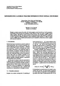
The numerical accuracy of Equation 21 can be improved using an iterative scheme, e.g. S0 = A0 = 1 1+k z Ak+1 = Ak × 2+k 1 21 + k Sk+1 = Sk + Ak+1 ˜ and G(z) ≈ 2zSK for large enough K. In practice however we prefer to use a large multi-resolution look-up table of precomputed values obtained from a numerical-package. As shown in Figure 1, this function decreases very slowly as its argument becomes increasingly negative, so we can easily compute accurate ˜ evaluations of G(z) for any z by linear interpolation of our lookup table and, as a by-product, we also obtain ˜′. G We have now defined all the terms in the bound L. 4.4

−8

Optimising The Bound

To perform inference we optimise the variational parameters m, S and the model parameters Θ to maximise L. To optimise these simultaneously we construct an augmented vector y = [Θ⊤ , m⊤ , vech(L)⊤ ]⊤ —where vech(L) is the vectorisation of the lower triangular elements of L, such that S = LL⊤ . The necessary derivatives are presented in the appendix.

−800

−700

−600

−500

z

−400

−300

−200

−100

0

˜ can be obtained Figure 1: Accurate evaluations of G from a precomputed look-up table.

We can compute the maximum-likelihood (ML) solution by optimising L(D; y) or the maximum-aposterior (MAP) estimate by maximising L(D; y) + log p(Θ). (In principle we could also marginalise Θ numerically.) 4.5

Locating The Inducing Points

One final part of our model we have so far left unspecified is the number and location of inducing points. In principle, for a given set of parameters Θ, we will obtain a lower bound for the true GP likelihood for any number of inducing points in any configuration of locations. In practice, we distribute the inducing points evenly across the domain; we do this for two reasons. The first is because—in contrast to standard GP regression— the accuracy of our solution is not simply governed by the distance between the inducing points and the data points. The variance of f (x) increases as x gets further from the inducing points. However the expectation of λ is a function of both the mean and the variance of f . Since we are integrating this variance over the whole domain, we need to reduce the variance at all locations in the domain. This can can be achieved with an evenly-spaced grid. The second reason is that using regularly sampled grids provides computational advantages. When the grid points are evenly spaced, the kernel matrix has Toeplitz structure, and hence allows matrix inversion (and linear solving) in O(M log2 M ) time, a fact previously utilised for efficient point processes by Cunningham et al. (2008). Furthermore, when the kernel function is separable across the dimensions (as specified by (8)), the kernel matrix has Kronecker structure which


can further reduce the cost of matrix inversion Osborne et al. (2012). The latter is relevant to all sparse GP applications based on inducing points, however, it is particularly relevant for this application as we are motivated by the doubly intractable nature of Equation 3. In our implementation, we use na¨ıve inversion of the inducing point kernel matrix, Kuu , resulting in computational complexity of O(N M 3 ). Hence the impressive computation times reported below can be readily improved with a small amount of additional implementation effort.

5

ALTERNATIVE GP TRANSFORMATIONS

The square transform is not a one-to-one function; any rate function λ may have been generated by f 2 or (−f )2 . We can, however, break this non-identifiability using a prior or other means to bias f towards the positive (or indeed negative) solution.

6

At this point it is worth considering why we have chosen the function transformation λ(x) = f 2 (x) in preference to other alternatives we might have used. An obvious first choice would be λ(x) = exp f (x) . (22)

This transformation is undesirable for two reasons. The more obvious of these is that after taking expectations under q(f ) we are left with the integral Z σx2 − exp µx + dx (23) 2 T

which we cannot be computed in closed form. We could approximate the integral using a series expansion, however this would be very difficult with more than a couple of terms and furthermore, since the function is concave, this approximation would not be a lower bound. The second—and more subtle—reason is that in using this transformation, when we take expectations under q(f ) of the data, we obtain Eq(f ) [log {exp(fn )}] = µn .

In contrast the square transform presented allows the integral over the region T to be computed in closed form and Eq(f ) [log fn2 ] can be computed very quickly and accurately. Importantly this transformation also maintains the connection between the data and the variational uncertainty.

(24)

Since the mean, µn , is not a function of S, the variance of the variational distribution q(u), we have effectively decoupled the data from the uncertainty on our variational approximation; this is clearly undesirable. Another possible candidate is the probit function, λ(x) = Φ(f (x)). This can be integrated analytically against the GP prior, however we are again left with a difficult integral over T which is ! Z µx dx. (25) Φ p − 1 + σx2 T

As the range of this transformation is (0, 1) we would also require additional machinery to infer a scaling variable.

EXPERIMENTS

To evaluate our algorithm, we benchmarked against a frequentist kernel smoothing (KS) approach and a fully Bayesian SGCP MCMC sampler. Our test data sets are generative data from the SGCP model and several real-world data sets. For the synthetic data sets, we first generate a function from a high resolution grid, and then, conditioned on that function, we draw a training dataset and multiple test data sets. We give average and worst case performance for these test data sets. For the real-world data we either: sub-sample without replacement a Poissondistributed number of points; or allocate each point into a test set with probability 0.5, else it is allocated to the training set. For our VBPP algorithm, we present two test loglikelihood numbers. The first is simply the lower bound, L(H ; y∗ ), evaluated with the learned parameters and the test data set H = {˜ x(k) }K k=1 . However, since this bound is not very tight, we find that we do not achieve particularly good predictive likelihoods. To tighten the bound, we therefore adopt the following strategy: having learned the model and variational parameters as before, we take the mean of the variational distribution, i.e. E[q(u)] = m, and treat m as a model parameter, that is, we discard its associated uncertainty; this allows us to set S = 0. Under this interpretation m is no longer a random variable with a prior and a posterior, and so we can also set KL(q(u)||p(u)) = 0. We can now re-evaluate the bound which we now denote L0 . In essence the strategy is to use only the mean of the GP posterior to construct our rate function, however we limit this hard decision to the inducing points (therefore f (x), x 6∈ Z, is still a random function). 6.1

Benchmarks

Our kernel smoothing method is similar to standard kernel density estimation except we use truncated normal kernels to account for our explicit knowledge of the


domain—the latter is referred to as “end-correction” in some literature (Diggle, 1985). The kernel smoother optimises a diagonal covariance, Σ∗ , by maximising the leave-one-out training objective Σ∗ = argmax Σ

N X

log

N X

j6=i=1

i=1

NT (x(i) ; x(j) , Σ).

(26)

We can construct the predictive distribution by combining the maximum-likelihood estimates of the size and spatial location of the point process. For the test data set H (with K! permutations) this distribution is p(H |D) = K! p(K|D)

K Y

k=1

p(˜ x(k) |D)

VB(L) intensities is small, the predictive log-likelihood and RMS error metrics in Tables 1 — 4 are significantly better in the L0 case. In general it is clear that the variational method performs approximately equivalently to the SGCP in the majority of cases, and typically surpasses the results delivered by both KDE methodologies. VBPP arrives at a full posterior over the function in a fraction of the time the SGCP does, albeit typically slightly slower than the maximum-likelihood solution delivered by KDE.

(27)

where the location density p(˜ x(k) |D) =

N 1 X NT (˜ x(k) ; x(n) , Σ∗ ) N n=1

(28)

is computed using using the previously described method and the distribution of the number of points K

p(K|D) =

N exp(−N ) K!

(29)

is simply a Poisson distribution with parameter N . It is straight forward to show that Equation 27 is equivalent to Equation 1 since we can interpret the rate function as λ(x) =

N X

n=1

and since

R

T

NT (x; x(n) , Σ∗ )

(30)

λ(x)dx = N .

Our SGCP sampler is based on (Adams et al., 2009). Our implementation differs by using elliptical slice sampling to infer the latent functions function f and we perform hyper-parameter inference using Hybrid Monte-Carlo (HMC). We also use the “adaptivethinning” method described in (Gunter et al., 2014a) reduce the number of thinning points required. 6.2

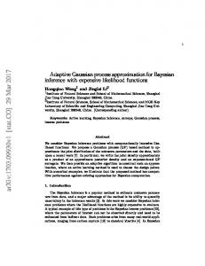
Figure 2: 2D Synthetic Data. Clockwise from top left: Ground truth, VBPP, KDE+EC, SGCP.

Synthetic Data

As an early test, we first draw generative 1D and 2D data from the SGCP, which is a generative model similar to the VBPP. We then attempt to recover the underlying intensity function, using our own approach (VBPP), KDE with end correction (KDE+EC), KDE without end correction (KDE-EC), and the SGCP. Conditioned on ∼ 80 observations, Figures ?? and 2 visualise the inferred intensities: It can be seen in the 1D case that while the difference between the VB(L0) and

6.3 6.3.1

Real Data Coal Mining Disaster Data

Our first real dataset comprises 190 events recorded from March 15, 1851 to March 22, 1962; each represents a coal-mining disaster that killed at least ten people in the United Kingdom. These data, first analysed in this form by (Jarrett, 1979), have often been tackled with nonhomogeneous Poisson processes (Adams et al., 2009) as the rate of such disasters is expected to vary according known historical developments. The events are indicated by the rug plot along the axis of Figure 3. Our inferred intensity of disasters correlates with the historical introduction of safety regulation, as noted in previous work on this data (Fearnhead, 2006; Carlin et al., 1992). Firstly, our results depict a decline in the rate of such disasters throughout 1870–1890, a period that saw the UK parliament passing several acts with the aim of improving safety for mine workers, including the Coal Mines Regulation Acts of 1872 and 1887. Our inferred intensity also declines after 1950, likely related to the imposition of further safety regulation with the Mines and Quarries Act, 1954. Predictive log-likelihood on held out data (Table 5) are also encouraging, suggesting that it is an appropriate model in this case.

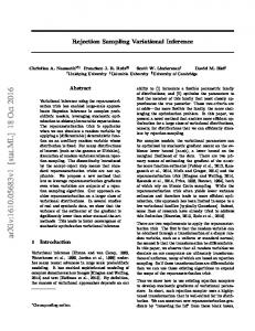
Chris Lloyd* , Tom Gunter* , Michael A. Osborne, Stephen J. Roberts Coal Mining Disaster Data

Twitter MP Data 20 18 16 14 12 10 8 6 4 2 0 0

Data VB(L) VB Var VB (L0 ) KS+EC KS-EC SGCP

Tweets

Deaths per Year

2 1.8 1.6 1.4 1.2 1 0.8 0.6 0.4 0.2 0

1860

1880

1900 1920 Year

1940

1960

Figure 3: Coal mining disaster data.

Function 1 2 3 4

Function 1 2 3 4

Function 1 2 3 4 5

1 2 3 4 5

5

Day

10

15

Figure 4: 1D Twitter Data.

Table 1: Test log-likelihood for 1D synthetic data. SGCP KDE-EC KDE+EC VBPP (L) Avg. Min Avg. Min Avg. Min Avg. Min

VBPP (L0 ) Avg. Min

209.7 68.3 4.2 -3.0

207.1 64.9 5.1 -3.6

148.8 41.0 -4.4 -8.7

202.3 61.1 0.2 -7.1

147.4 32.8 -7.9 -13.5

207.3 65.4 3.5 -3.0

151.8 36.4 -4.7 -9.9

199.4 52.0 -0.2 -4.2

144.3 23.0 -8.9 -9.6

Table 2: RMS error and wall-clock time for 1D synthetic data. SGCP KDE-EC KDE+EC VBPP (L) RMS Time(s) RMS Time(s) RMS Time(s) RMS Time(s) 2.6 1.0 1.3 0.7

Function

Data VB(L) VB Var VB(L0 ) KS+EC KS-EC SGCP

124.7 120.5 112.2 108.1

3.9 3.1 1.4 1.1

0.022 0.003 0.002 0.003

3.3 2.7 1.5 0.9

0.016 0.005 0.003 0.004

3.2 2.9 1.2 0.8

0.7 0.6 0.6 0.6

151.7 35.8 -3.7 -9.0

VBPP (L0 ) RMS Time(s) 3.2 2.8 1.1 0.8

0.7 0.6 0.6 0.6

Table 3: Test log-likelihood for 2D synthetic data. SGCP KDE-EC KDE+EC VBPP (L) Avg. Min Avg. Min Avg. Min Avg. Min

VBPP (L0 ) Avg. Min

446.1 -61.1 122.4 175.8 446.1

392.9 -76.1 92.6 148.3 415.5

398.1 -73.6 73.7 137.6 365.0

333.8 -109.0 43.6 111.9 369.5

292.8 -123.3 -3.2 81.4 305.6

389.8 -78.3 84.3 147.0 413.6

347.5 -91.7 33.8 111.9 345.1

355.9 -91.0 64.2 93.6 354.0

310.4 -102.1 15.5 61.7 285.7

347.2 -87.3 43.4 115.2 346.9

Table 4: RMS error and wall-clock time for 2D synthetic data. SGCP KDE-EC KDE+EC VBPP (L) RMS Time(s) RMS Time(s) RMS Time(s) RMS Time(s)

VBPP (L0 ) RMS Time(s)

1.37 0.38 0.88 1.71 2.94

1.21 0.38 0.81 1.14 1.81

7547.83 1039.65 3173.91 3773.75 6368.44

2.01 0.66 1.30 1.49 2.29

0.10 0.01 0.02 0.02 0.05

1.48 0.46 1.04 1.26 2.02

0.34 0.02 0.12 0.05 0.21

1.21 0.36 0.81 1.11 1.82

3.26 2.00 2.44 2.58 2.83

3.26 2.00 2.44 2.58 2.83


Table 5: Results for Coal Mining Disaster Data

6.3.2

METHOD

LOG-LIKE

TIME(s)

VBPP (L) VBPP (L0 ) KS+EC KS-EC SCGP

-100.3 -92.2 -92.6 -95.9 -96.9

0.7 0.7 0.0 0.0 417.6

Table 7: Test log-likelihood for 1D Twitter data.

Malaria Data

We expect that a major application of the contributions presented in this paper is the joint modelling of disease incidence with correlating factors, in a fully Bayesian, scalable framework. For example, those studying the spread of Malaria often wish to use continuous rainfall measurements to better inform their epidemiological models.

Figure 5: Malaria incidences in Kenya. We use examples from the Malaria Atlas Project (map, 2014) to test our scheme. Specifically, we extract 733 incidences of Malaria outbreak documented in Kenya between 1985 and 2010, and run all algorithms excluding the SGCP on half of the resulting dataset, holding out the remainder for testing. Table 6 gives the held out test log-likelihood for the four schemes. Table 6: Test log-likelihood for 2D Malaria data. KDE-EC

KDE+EC

VBPP(L)

VBPP(L0 )

199.1

224.0

332.1

416.6

6.3.3

Darling, one week either side of the Scottish independence election. Results are shown in Figure 4 and Table 7, where as ever half the data was held out for testing.

Twitter Data

Finally, we ran the models on the tweet profile of the chairman of the ‘Better Together Campaign’, Alistair

7

METHOD

TEST L-L

RUN TIME (S)

VBPP (L) VBPP (L0 ) KS+EC KS-EC SCGP

51.0 67.3 67.4 65.4 68.1

0.5 0.5 0.3 0.2 230.0

FURTHER WORK

Although the performance of the variational Bayesian point process inference algorithm described in this paper improves upon standard methods when used in isolation, it is in its extensions that its utility will be fully realised. Previous work (Gunter et al., 2014a) has shown that hierarchical modelling of point processes— structured point processes—can significantly improve predictive accuracy. In these multi-output models, statistical strength is shared across multiple rate processes via shared latent processes. The method presented here provides a likelihood model for pointprocess data that can be incorporated as a probabilistic building-block into these larger interconnected models. That is, our fully generative model can readily be extended to additionally incorporate other observation modalities. For example, real-valued observations such as (log-) household income could be modelled along with the intensity function over crime incidents using a variational multi-output GP framework. Future work will be aimed towards developing these variational structured point process algorithms and integration of these techniques to popular Gaussian process tool-kits, such as GPy (the GPy authors, 2014).

8

CONCLUSION

Point process models have hitherto been hindered by their scaling with the number of data. To address this problem, we propose a new model, accommodating non-discretised intensity functions, that permits linear scaling. We additionally contribute a variational Bayesian inference scheme that delivers rapid and accurate prediction. The scheme is validated on real datasets including the canonical coal mining disaster data set and data describing Malaria incidences in Kenya.


References Malaria Atlas Project. http://www.map.ox.ac.uk/ explore/data-modelling/, 2014. [Online; accessed 24-October-2014]. R. P. Adams, I. Murray, and D. J. C. MacKay. Tractable Nonparametric Bayesian Inference in Paussian Processes with Gaussian Process Intensities. In Proceedings of the 26th Annual International Conference on Machine Learning, ICML ’09, pages 9–16, New York, NY, USA, 2009. ACM.

R. G. Jarrett. A note on the intervals between coalmining disasters. Biometrika, 66(1):191193, 1979. doi: 10.1093/biomet/66.1.191. J. F. C. Kingman. Paussian Processes (Oxford Studies in Probability). Oxford University Press, jan 1993. ISBN 0198536933. Jesper Mller, Anne Randi Syversveen, and Rasmus Plenge Waagepetersen. Log Gaussian Cox Processes. Scandinavian Journal of Statistics, 25(3): 451–482, 1998. ISSN 1467-9469.

L. U. Ancarani and G. Gasaneo. Derivatives of any order of the confluent hypergeometric function 1 F1 (a, b, z) with respect to the parameter a or b. Journal of Mathematical Physics, 49(6), 2008.

M. A. Osborne, S. J. Roberts, A. Rogers, and N. R. Jennings. Real-time information processing of environmental sensor network data. ACM Transactions on Sensor Networks, 9(1), 2012. doi: 10.1145/ 2379799.2379800.

Sankarshan Basu and Angelos Dassios. A cox process with log-normal intensity. Insurance: Mathematics and Economics, 31(2):297302, Oct 2002. doi: 10. 1016/S0167-6687(02)00152-X.

C. E. Rasmussen and C. K. I. Williams. Gaussian Processes for Machine Learning. The MIT Press, 2nd edition 2006 edition, 2006. ISBN 0-262-18253X.

Bradley P. Carlin, Alan E. Gelfand, and Adrian F. M. Smith. Hierarchical Bayesian analysis of changepoint problems. Journal of the Royal Statistical Society. Series C (Applied Statistics), 41(2):389405, Jan 1992.

Stephen L. Rathbun and Noel Cressie. Asymptotic properties of estimators for the parameters of spatial inhomogeneous Paussian point processes. Advances in Applied Probability, page 122154, 1994.

John P. Cunningham, Krishna V. Shenoy, and Maneesh Sahani. Fast Gaussian process methods for point process intensity estimation. In Proceedings of the 25th international conference on Machine learning, pages 192–199. ACM, 2008. P. Diggle. A kernel method for smoothing point process data. Journal of the Royal Statistical Society. Series C (Applied Statistics), 34(2):pp. 138–147, 1985. ISSN 00359254. Paul Fearnhead. Exact and efficient Bayesian inference for multiple changepoint problems. Statistics and Computing, 16(2):203213, Jun 2006. doi: 10.1007/ s11222-006-8450-8. Tom Gunter, Chris Lloyd, Michael A. Osborne, and Stephen J. Roberts. Efficient Bayesian Nonparametric Modelling of Structured Point Processes. 2014a. Tom Gunter, Michael A. Osborne, Roman Garnett, Philipp Hennig, and Stephen Roberts. Sampling for inference in probabilistic models with fast Bayesian quadrature. In C. Cortes and N. Lawrence, editors, Advances in Neural Information Processing Systems (NIPS), 2014b. Juha Heikkinen and Elja Arjas. Modeling a Paussian forest in variable elevations: A nonparametric Bayesian approach. Biometrics, 55(3):738745, Sep 1999.

Maneesh Sahani, M. Yu Byron, John P. Cunningham, and Krishna V. Shenoy. Inferring neural firing rates from spike trains using Gaussian processes, page 329336. 2007. the GPy authors. GPy: A Gaussian process framework in python. https://github.com/SheffieldML/ GPy, 2014.

Appendix The derivative of the bound with respect to the variational parameters m and vech(L), S = LL⊤ are: ∂L −1 −1 = −2K−1 uu ΨKuu m − Kuu m ∂m N 2 X ˜ ′ − µn µn knu K−1 G + uu 2σn2 σn2 n=1

∂L 1 −1 −1 = Tr(K−1 Kuu − S−1 uu ΨKuu ) − ∂S 2 N 2 X 1 1 ˜ ′ − µn + −G + 2σn2 2σn4 σn2 n=1 −1 × K−1 uu kun knu Kuu ∂L ∂L ∂S dL = × = 2 vech L ∂vech(L) ∂S ∂vech(L) dS