A General Diagnostic Model Applied to Language Testing Data - ETS

Research Report

A General Diagnostic Model Applied to Language Testing Data

Matthias von Davier

Research & Development

September 2005 RR-05-16

A General Diagnostic Model Applied to Language Testing Data

Matthias von Davier ETS, Princeton, NJ

September 2005

As part of its educational and social mission and in fulfilling the organization's nonprofit charter and bylaws, ETS has and continues to learn from and also to lead research that furthers educational and measurement research to advance quality and equity in education and assessment for all users of the organization's products and services. ETS Research Reports provide preliminary and limited dissemination of ETS research prior to publication. To obtain a PDF or a print copy of a report, please visit: http://www.ets.org/research/contact.html

Copyright © 2005 by Educational Testing Service. All rights reserved. EDUCATIONAL TESTING SERVICE, ETS, the ETS logo, and TOEFL are registered trademarks of Educational Testing Service. The Test of English as a Foreign Language is a trademark of Educational Testing Service.

Abstract Probabilistic models with more than one latent variable are designed to report proles of skills or cognitive attributes. Testing programs want to oer additional information beyond what a single test score can provide using these skill proles. Many recent approaches to skill prole models are limited to dichotomous data and have made use of computationally intensive estimation methods like the Markov chain Monte Carlo (MCMC), since standard maximum likelihood (ML) estimation techniques were deemed infeasible. This paper presents a class of general diagnostic models (GDMs) that can be estimated with customary ML techniques and applies to polytomous response variables as well as to skills with two or more prociency levels. The model and the algorithm for estimating model parameters handles directly missing responses without the need of collapsing categories or recoding the data. Within the class of GDMs, compensatory as well as noncompensatory models may be specied. This report uses one member of this class of diagnostic models, a compensatory diagnostic model that is parameterized similar to the generalized partial credit model (GPCM). Many well-known models, such as uni- and multivariate versions of the Rasch model and the two parameter logistic item response theory (2PL-IRT) model, the GPCM, and the FACETS model, as well as a variety of skill prole models, are special cases of this member of the class of GDMs. This paper describes an algorithm that capitalizes on using tools from item response theory for scale linking, item t, and parameter estimation. In addition to an introduction to the class of GDMs and to the partial credit instance of this class for dichotomous and polytomous skill proles, this paper presents a parameter recovery study using simulated data r and an application to real data from the eld test for TOEFL° Internet-based testing (iBT).

Key words: Cognitive diagnosis, item response theory, latent class models, EM-algorithm

i

1. Introduction and Overview The goal of this paper is to introduce a class of general diagnostic models suggested by von Davier and Yamamoto (2004c) and to provide evidence that an instance of this class of general diagnostic models (GDMs), the GDM for partial credit data, is capable of accurate parameter recovery for models with multivariate skill variables. The second goal of this report is to present results using this GDM for partial credit data (subsequently referred to as pGDM) for r analyzing TOEFL° Internet-based testing (iBT) Reading and Listening data from two test forms,

subsequently referred to as Form A and Form B. The third goal is to discuss how results from the pGDM compare to standard item response theory (IRT) models and to provide information to aid in improving on the specication of the Q-matrix used in cognitive diagnosis models. Cognitive diagnosis models for skill prole reporting have received a lot of attention in recent years. Early work by Tatsuoka (1983) was based on IRT and a classication of aberrant response patterns. Other roots of cognitive diagnosis can be found in work that extends latent class analysis (LCA; Lazarsfeld & Henry, 1968) to approaches that allow more than one latent variable. The aim of these diagnostic models is to identify skill proles, that is, to perform multiple classications of examinees based on their observed response patterns with respect to features (skills/attributes) that are assumed to drive the probability of correct responses. The approach taken here denes a general class of models for cognitive diagnosis (GDM) based on extensions of latent class models, the Rasch model, item response theory models, as well as skill prole models. Skill prole models may be used by testing programs that want to oer additional information beyond what a single test score provides. Many recent approaches are using computationally intensive estimation methods like Markov chain Monte Carlo (MCMC), since standard maximum likelihood (ML) estimation techniques were either unavailable or were deemed infeasible. von Davier and Yamamoto (2004a, 2004b) suggested a class of GDMs and outline parameter estimation for these models using standard ML techniques. The class of GDMs extend the applicability of skill prole models to polytomous items and to skills with more than two prociency levels. Within the GDMs, compensatory as well as noncompensatory models may be specied. An instance of this class, the pGDM contains many well-known models, such uni- and multivariate versions of the Rasch model (Rasch, 1960), the two parameter logistic item response theory (2PL-IRT) model (Birnbaum, 1968), the generalized partial credit model (GPCM; Muraki, 1992), and the FACETS model (Linacre, 1989), as well as a variety of skill prole approaches like multiple classication 1

LCA and a compensatory fusion model as special cases. An EM-algorithm for estimating the pGDM was recently implemented in the mdltm software developed by the author of this report. This implementation enables one to use standard tools from IRT for scale linking, for deriving measures of model t, item and person t, and for parameter estimation. The following section presents an introduction to the class of GDMs for dichotomous and polytomous skill proles. Following this, the GDM is specialized to an instance of this class, the pGDM. Subseqent sections present applications of the pGDM to simulated data and to real data from the TOEFL iBT program. The examples using simulated data show the pGDM's capability of recovering parameters from simulated multivariate item response data with an associated Q-matrix. The application to the TOEFL iBT data is based on a comparison of diagnostic skill prole models for two subscales, Reading and Listening, making use of two test forms, Form A and Form B, with univariate and multivariate IRT approaches.

2. A Class of General Diagnostic Models Previous approaches to cognitive diagnosis modeling can be summarized as being based on one or more of a number of techniques, including the rule space methodology (Tatsuoka, 1983), latent class analysis (Haberman, 1979; Haertel, 1989; Maris, 1999), MCMC estimation of the (reparameterized) unied model (i.e., the fusion model implemented in the Arpeggio software; DiBello, Stout, & Roussos, 1995; Hartz, Roussos, & Stout, 2002), and discrete skill models estimated with Bayesian inference networks (BINs; e.g., Almond & Mislevy, 1999). The general class of GDMs as presented below was developed with the goal of maintaining similarities to these previous approaches using ideas from IRT, log-linear models, and latent class analysis. One central idea behind diagnostic models is that dierent items tap into dierent sets of skills or examinee attributes and that experts can generate a matrix of relations between items and skills required to solve these items. The matrix is commonly referred to as the Q-matrix, and it is an explicit building block in many of the diagnostic modeling approaches mentioned above. The general class of GDMs is instantiated in section 2.2 below to dene the pGDM, which contains many well-known IRT models as special cases. At the same time, the pGDM extends these models to multivariate, polytomous skill prole models (compare von Davier & Yamamoto, 2004c). Like many of the other contenders listed above, the class of GDMs makes use of a Q-matrix as an integral part of the model, but in its general form allows noninteger entries as well 2

as polytomous item responses and polytomous attributes/skills. The skill by item relations dened by a Q-matrix is also a central building block of the class of GDMs. However, the class of GDMs allows generalized versions of the Q-matrix, and more important, provides a more general approach of specifying how skill patterns and the Q-matrix interact than previous approaches. The GDM will be introduced in its general form in the next section, and following that, a specialized form of the GDM will be introduced in section 2.2 that already contains many well-known psychometric models.

2.1 Loglinear Class of Diagnostic Models This section introduces one particular way to formalize the class of GDMs for polytomous data and dichotomous or polytomous skill levels. The class of diagnostic models is dened by a discrete, multidimensional, latent variable θ, that is, θ = (a1 , . . . aK ), with discrete user-dened skill levels ak ∈ {sk1 , . . . , skl , . . . , skLk }. In the most simple (and most common) case the skills are dichotomous, that is, the skills will take on only two values, ak ∈ {0, 1}. In this case, the skill levels are interpreted as mastery (1) versus nonmastery (0) of skill k . Let θ = (a1 , .., aK ) be a

K -dimensional skill prole consisting of polytomous skill levels ak ,

k = 1, .., K . Then dene the

item specic logit as

· log

¸ P (X = x | βi , qi , γi , a) T = βxi + γxi· h(qi , a) P (X = 0 | βi , qi , γi , a)

(1)

with Q-matrix entries qi· = (qi1 , .., qiK ) and qik =∈ {0, 1, 2, . . .} for k = 1, .., K . In addition there are real valued diculty parameters βix and a k -dimensional slope parameter γxi = (γxi1 , .., γxiK ) for each nonzero response category x ∈ {1, 2, .., mi }. The model decomposes the conditional probability of a response x on item i into two summands, the overall diculty βxi , and a linear combination of skill level by Q-matrix terms h(qi· , a) = (h1 (qi· , a), . . . , hk (qi· , a)). Given a nonzero Q-matrix entry, the slopes γix· in the linear expression above determine how much the particular skill components in a = (a1 , .., aK ) contribute to the response probabilities for item i. The Q-matrix entries qik relate item i to skill k and determine whether (and to what extent) skill k is required for item i. If skill k is required for item i, then qik > 0; if skill k is not required, then qik = 0. Often, it implies that if skill k is dened as not required for item i in the Q-matrix by qik = 0, then skill level ak does not contribute at all to the response probabilities for this item.

3

The h(qi· , a) 7→ R are a central building block of the GDM. Giving these functions a specic form denes instances of the class of GDMs with specic properties, see section 2.2. The h mapping projects the skill-levels ak a = (a1 , .., aK ) using the Q-matrix entries qi· . In most cases, the same projection will be adopted for all items. The h are mappings that specify how Q-matrix entries determine the skill patterns impact on the condional response probabilities P (X = x|βi , qi , γi , a). The next subsection presents examples of such projections.

2.11 Instances of Skill by Q-Matrix Projections One particular choice of a mapping hi () relates the GDM to discrete, multivariate IRT models. The choice of h for IRT type models is

h(qi· , a) = (qi1 a1 , . . . , qiK aK )

(2)

so that the k -th component of h is hk (qi· , a) = qik ak . For q ∈ {0, 1}, is equivalent to

  a f or q = 1 k ik . hk (qi· , a) =  0 f or q = 0 ik

In this case, only the skills k with nonzero Q-matrix entries qik (the skills required for this item) contribute to the response probabilities P (x|βi , qi , γi , a) of item i. If qik = 1, there is a total contribution of γik h(qik , ak ) = γik ak for skill k in Equation 1. The above choice is appropriate for Q-matrices with 0/1 entries combined with various skill level choices. Skill levels like ak ∈ {−m, . . . , 0, . . . , +m} or mastery/nonmastery dichotomies like

ak ∈ {0, 1} may be used with this denition of h, as long as the Q-matrix contains only 0/1 entries. However, this choice of h(·) does not work well with Q-matrices that have entries other than

0/1. This is particularily true if the γ parameters as given in Equation 1 are to be estimated. In cases with integer or real valued Q-matrices, a useful choice is

hk (qik , ak ) = min(qik , ak )

(3)

for all k , with q ∈ {0, 1, 2, . . . , m} as well as a ∈ {0, 1, 2, . . . , m}. This coincides with the denition in 2 if q ∈ {0, 1}and a ∈ {0, 1}but diers in cases using arbitrary skill levels a or Q-matrix entries q .

4

The rationale of this particular choice of the minimum of q and a is that the GDM may be used for skills assessment where the Q-matrix entries represents a sucient level for skill k on item

i. A higher skill level than qik will not increase the probability of solving item i, whereas a skill level lower than qik results in a lower probability of solving item i.1

2.12 Examples of Skill Level Denitions for Various Models Assume that the number of skill levels is Sk = 2 and choose skill levels ak ∈ {−1.0, +1.0}, or alternatively, ak ∈ {−0.5, +0.5}. Note that these skill levels are a-priorily dened constants and not model parameters. This setting can be easily generalized to polytomous, ordinal skills levels with the number of levels being Sk = m + 1 and a determination of levels like ak ∈ {(0 − c), (1 − c), . . . , (m − c)} for some constant c, an obvious choice is c = m/2. Consider a case with just one dimension, say K = 1,, and many levels, say Sk = 41, with levels of ak being equally spaced (a common, but not a necessary choice), say ak ∈ {−4.0, . . . , +4.0}. Here, the GDM mimics a unidimensional IRT model, namely the GPCM (Muraki, 1992).

2.13 The Class of Diagnostic Model in Logistic Form The loglinear formulation of the class of GDMs as given in Equation 1 may be transformed to a logistic form that is more familiar to researchers working with IRT models. The model as introduced above is equivalent to

£ ¤ T h(q , a) exp βxi + γxi· i h i P (X = x | βi , qi , γi , a) = P i T h(q , a) exp β + γ 1+ m yi i y=1 yi·

(4)

P with k -dimensional skill prole a = (a1 , .., aK ) and with some necessary restrictions on the k γxik P and βxi to identify the model. Using this reformulation and further speciying the mapping h() shows that a particular instance of the GDMs already contains common IRT models and a compensatory fusion model as special cases. The parameters βxi as well as γxik may be interpreted as threshold and slope parameters, respectively.

5

2.2 A General Diagnostic Model for Partial Credit Data One particular member of the class of GDMs is chosen for the subsequent analyses. The choice of hk (qi· , a) = qik ak together with Q-matrices containing only 0/1 entries leads to a model that retains many features of well-known IRT models while extending these models to diagnostic applications with multivariate latent skills. In addition, the slope parameters are subject to the constraint γixk = xγik , so that the resulting instance is a GDM for dichotomous and polytomous pGDM. Skill prole models such as multiple classication latent class models (Maris, 1999), located latent class models (Formann, 1985), and a compensatory version of the fusion model (Hartz et al., 2002) are special cases of the pGDM. This model is suitable for dichotomous and ordinal responses

x ∈ {0, 1, 2, .., mi }. Given the above denitions, h i P exp βxi + K xγ q a ik ik k k=1 h i P (X = x | βi , a, qi , γi ) = Pmi PK 1 + y=1 exp βyi + k=1 yγik qik ak

(5)

with k attributes (discrete latent traits) a = (a1 , .., aK ), and a dichotomous design Q-matrix

(qik )i=1..I,k=1..K . The ak are discrete scores determined before estimation and can be chosen by the user. These scores are used to assign real numbers to the skill levels, for example a(0) = −1.0 and a(1) = +1.0 may be chosen for dichotomous skills (see section 2.12). de la Torre and Douglas (2004) estimated the dichotomous version of this model, the linear logistic model (LLM; Maris, 1999; Hagenaars, 1993), using MCMC methods. For ordinal skills with sk levels, the ak may be dened using a(x) = x for x = 0, . . . , (sk − 1) or a(0) = −sk /2, . . . , a(sk − 1) = sk /2 (see section 2.12). The parameters of the models as given in Equation 5 can be estimated for dichotomous and polytomous data, as well as for ordinal skills, using the EM-algorithm. The process of instantiation from the general class of GDMs to the pGDM and its specialization to commonly used IRT models is illustrated in Table 1. The examples of instantiation from the general class of GDMs down to a discrete version of the common 2PL or GPCM, or a skill model with k-dimensional skill-patterns with dichotomous components as used in the analyses below in Table 1, show how dierent choices of a Q-matrix and a skill by item mapping h() lead to certain models. von Davier and Yamamoto (2004c) presented other examples of instantiations that show that located latent class models and a compensatory fusion model version can be specied within the pGDM.

6

Table 1 Instantiation From a General Class of Models to a pGDM Model/Class The class of GDMs Compensatory GDMs pGDM Example: 2PL or GPCM Example: k-skill model

Mapping h(q, a) h ((qi1 , ..qiK ) , (a1 , ..aK )) h (qik , ak ) see section 2.11 h (qik , ak ) = qik ak h (qi , a) = 1a = θ(a) see section 2.12 h(qi , a) = qik a with a ∈ {−1, 1}

Q-matrix real valued I × K real valued I × K zeroes/ones I × K vector of ones I × 1 zeroes/ones I × K

2.3 Estimation and Data Requirements An implementation of marginal maximum likelihood (MML) parameter estimation using the EM-algorithm for the pGDM, as given in Equation 5, was developed by the author of this report. This algorithm is based on a previous program for estimating the parameters of discrete mixture distribution IRT models (von Davier, 2001; von Davier & Yamamoto, 2004c). This extended program, called mdltm, provides information about convergence of parameter estimates, numbers of required iteration cycles and descriptive measures of model-data t and item t. The mdltm program is controlled by a scripting language that describes the data input format, the Q-matrix, and other features of the cognitive skill model (i.e., the number of skill levels and skill level scores

ak for each skill and whether the γ parameters are constrained across items or estimated freely). The mdltm software has been tested with samples of up to 200,000 examinees, when implementing a conrmatory two-dimensional 2PL IRT model. Other trials included up to 50,000 examinees when implementing an eight-dimensional dichotomous skill model [θ = (a1 , . . . , a8 ) with

ak ∈ {−1, 1}]. Larger numbers of skills very likely pose problems with identiability, no matter whether MCMC (in Bayes nets or other approaches), or MML methods are used to estimate parameters, unless the number of items per skill variable is suciently large. For diagnostic models with that many skills, the mdltm software allows the specication of a number of constraints that may help to achieve identiability. At this point in time, the following diagnostic skill prole models can be estimated with the mdltm software:

• Multiple classication latent class models • A compensatory fusion/Arpeggio (sometimes referred to as the reparameterized unied) model • Extensions of these models to polytomous response data, and polytomous skill levels 7

• Rasch model, partial credit model, 2PL IRT (Birnbaum) model, GPCM, • Latent class analyses, conrmatory multivariate IRT, mixture IRT models The data requirements for the software are as follows: The software can read ASCII data les in arbitrary format; the scripting language used to control the software enables the user to specify which columns represent which variables. The software also handles weighted data, multiple group data (multiple populations), data missing by design (matrix samples) in response variables, and data missing at random in response variables, and missing data in grouping variables. The output is divided into a model parameter summary and an estimation summary, and a le that contains the scores and attribute classications for each examinee. This le also contains the percent correct for each subscale as dened by the Q-matrix and the examinee ID code.

3. Parameter Recovery for Skill Prole Data The following sections show how the pGDM recovers parameters for item response data with known skill by item relations (i.e., for a known Q-matrix). The example reported here is based on estimates from 40 simulated datasets with 36 items with a dichotomous response format and 2880 simulated examinees each. The model used to generate the data was based on four dichotomous skills. As input, the generating [36 × 4] Q-matrix was provided, that is, the item-skill relations were given as xed and known. The parameters were estimated using the mdltm software. The Q-matrix was generated randomly with a probability of p = 0.5 of a 1.0 entry in all cells of the Q-matrix. The diculty parameters were drawn from a normal N (0, 1) distribution and the slope parameters were drawn from a normal N (1, 0.25) distribution. The Q-matrix was the same across simulated datasets, as were the true skill patterns and the generating slope and diculty parameters. The generating (true) diculty and slope parameters are given on the left-hand side of Table 2. The generating probability distribution of the 16 dierent skill patterns is given in Table 4 in the truth column. The data were generated using the model equation in Equation 5. The following subsections present results based on a comparison of the estimated parameters and skill pattern distributions with the generating (true) values of these parameters.

3.1 Parameter Recovery Results The simulated datasets were generated using R (http://cran.r-project.org), the free S-Plus clone, and were analyzed using the mdltm software. 8

A script was written in R that allows the user to simulate item response data that follow a model according to Equation 5 with four dichotomous skill variables. Table 2 shows the generating slope parameters in places where the Q-matrix has a nonzero entry and contains -/- otherwise. The generating diculty parameters are given in the column denoted by βi on the left-hand side. The estimated parameters were subject to two constraints that match the data generating process. The mean of the diculties was assumed to be 0.0 and the mean of the slopes was assumed to be 1.0. If other constraints were used, the estimated parameters would have been subject to a transformation that has to be taken into account when estimating the accuracy of parameter recovery. Table 2 shows the root mean square errors (RSME) of the parameter estimates, that is,

v u 40 u1 X RM SE(ˆ α) = t (ˆ αi − αtrue )2 , 40

(6)

i=1

where αtrue is the generating value of the parameter, and α ˆ i is the estimate from the i-th dataset. Note that empty cell entries corresponding to a value of 0.0 in the Q-matrix are marked with -/-. The largest value for the RMSE is found for Item 34, RM SE(β34 ) = 0.154. This item, at the same time, has the most extreme item diculty parameter of the set, β34 = −3.611, so that a larger standard error of estimation as well as a slightly larger bias may be expected. The average 1 P ˆ i and the empirical standard error (s.e.) bias is dened as B(ˆ α) = αM − αtrue with αM = 40 iα is dened as

v u 40 u1 X s.e.(ˆ α) = t (ˆ αi − αM )2 . 40 i=1

Table 3 shows average bias and standardized residuals B(ˆ α)/s.e.(ˆ α) for parameter estimates. All residuals are of moderate size, and the RMSE values are homogeneous across items, for both the four slopes and the diculty parameters. None of the standardized residuals are larger than the critical value −3.5013 < z < 3.5013 based on a Bonferroni corrected α = 0.00046 = 0.05/108, assuming a normal distribution. Parameter estimates were not adjusted to match the overall mean (or log mean) of the generating parameter values, nor were the generating values used as starting values. The starting values for estimation were 0.0 for diculties and 1.0 for slopes. The starting distribution for the skill pattern probabilities were uniform. Taking the relative size of the bias into account, Tables 23 show that parameters are recovered accurately. 9

Table 2 Generating Parameters and RMSE of the Parameter Estimates Generating parameters Item i

γ1i

γ2i

γ3i

RMSE γ4i

βi

Item

γ1i

γ2i

γ3i

γ4i

βi

1

-/-

0.68692

-/-

0.73681

-1.07045

1

-/-

0.05953

-/-

0.06103

0.04161

2

-/-

0.33594

0.96009

-/-

-0.13508

2

-/-

0.06162

0.05761

-/-

0.03648

3

-/-

1.03094

0.77417

-/-

-0.28843

3

-/-

0.06090

0.05167

-/-

0.04048

4

0.87669

-/-

-/-

0.63231

-0.87271

4

0.05666

-/-

-/-

0.04889

0.04451

5

-/-

0.51326

1.24808

-/-

0.71665

5

-/-

0.05924

0.05770

-/-

0.06034

6

0.93370

-/-

-/-

1.06978

-0.22106

6

0.05847

-/-

-/-

0.06110

0.05577

7

-/-

-/-

-/-

-/-

0.91743

7

-/-

-/-

-/-

-/-

0.03563

8

1.24307

-/-

-/-

1.01998

1.66109

8

0.07454

-/-

-/-

0.08037

0.07791

9

1.37841

0.63066

0.89836

-/-

0.19979

9

0.07233

0.08324

0.06151

-/-

0.05685

10

-/-

1.12834

0.92587

1.13789

0.31114

10

-/-

0.07841

0.07709

0.06954

0.07409

11

-/-

-/-

-/-

-/-

1.12535

11

-/-

-/-

-/-

-/-

0.04219

12

-/-

0.96446

0.99007

-/-

0.58775

12

-/-

0.07359

0.05722

-/-

0.04856

13

-/-

0.74277

1.27635

0.77795

1.23988

13

-/-

0.07454

0.07526

0.08377

0.07887

14

-/-

-/-

-/-

0.96845

0.13247

14

-/-

-/-

-/-

0.04250

0.04442

15

-/-

-/-

0.96954

-/-

1.53576

15

-/-

-/-

0.07224

-/-

0.06791

16

1.48847

-/-

1.05186

0.76383

-0.11062

16

0.06806

-/-

0.07061

0.08617

0.05600

17

-/-

0.92499

0.67772

-/-

0.78303

17

-/-

0.05805

0.05022

-/-

0.04782

18

-/-

-/-

-/-

0.86182

0.10393

18

-/-

-/-

-/-

0.04472

0.04003

19

-/-

1.12678

0.60013

0.50905

0.57051

19

-/-

0.08038

0.05240

0.07592

0.06156

20

1.24929

-/-

1.02421

0.76603

0.57814

20

0.05599

-/-

0.07078

0.06801

0.05959

21

-/-

-/-

0.95400

0.80630

0.62558

21

-/-

-/-

0.06336

0.05392

0.05903

22

0.93378

-/-

-/-

1.10012

-0.73748

22

0.06005

-/-

-/-

0.05538

0.05365

23

-/-

0.91165

0.65792

1.36767

-0.77870

23

-/-

0.08028

0.08197

0.07804

0.08108

24

1.43815

-/-

1.04525

1.00269

1.61808

24

0.07542

-/-

0.09782

0.08237

0.10283

25

1.00611

-/-

-/-

0.98702

-0.65120

25

0.05312

-/-

-/-

0.05968

0.05477

26

0.84290

-/-

1.42168

-/-

1.10440

26

0.05632

-/-

0.08783

-/-

0.06681

27

1.06509

-/-

-/-

0.90191

0.06198

27

0.07064

-/-

-/-

0.07153

0.04237

28

-/-

0.91012

1.21093

-/-

0.20378

28

-/-

0.06652

0.06344

-/-

0.04931

29

1.04187

-/-

0.67220

-/-

0.32692

29

0.05840

-/-

0.05529

-/-

0.04268

30

1.03021

-/-

1.16820

0.99947

-0.76693

30

0.05670

-/-

0.06473

0.07367

0.05921

31

-/-

-/-

0.89491

-/-

-1.23301

31

-/-

-/-

0.05011

-/-

0.04170

32

-/-

1.08660

1.01277

-/-

-1.01561

32

-/-

0.07616

0.05341

-/-

0.06065

33

1.18379

0.72921

-/-

-/-

-0.93440

33

0.05262

0.06443

-/-

-/-

0.05061

34

-/-

-/-

1.13221

-/-

-3.61158

34

-/-

-/-

0.14869

-/-

0.15422

35

-

1.18415

0.91200

0.78920

-1.47219

35

-/-

0.08626

0.07967

0.07739

0.06818

36

0.64152

0.91027

0.94237

-/-

-0.50421

36

0.06647

0.07148

0.07556

-/-

0.06094

10

Table 3 Mean Bias and Standardized Residuals Mean bias Item i

γ1i

γ2i

Standardized residuals

γ3i

γ4i

βi

Item

γ1i

γ2i

γ3i

γ4i

βi

1

-/-

0.01106

-/-

-0.01609

0.00202

1

-/-

1.18112

-/-

-1.70698

0.30365

2

-/-

-0.01928

0.00202

-/-

0.00005

2

-/-

-2.05723

0.21924

-/-

0.01017

-/-

-0.00634

0.00817

-/-

-0.00509

3

-/-

-0.65402

1.00047

-/-

-0.79205

-/-

0.00552

0.00772

4

-0.94510

-/-

-/-

0.71030

1.10038

-/-

-0.00327

5

-/-

-0.50624

-1.06681

-/-

-0.33943

-0.01358

6

0.91533

-/-

-/-

0.55140

-1.56854

0.00023

7

-/-

-/-

-/-

-/-

0.04035

3 4

-0.00847

-/-

5

-/-

6

0.00848

-/-

-/-

0.00537

7

-/-

-/-

-/-

-/-

8

-0.00168

9

0.00774

-0.00478

-/-

-0.00971

-/-

0.00605

-0.01912

8

-0.14123

-/-

-/-

0.47195

-1.58099

-0.02729

0.00916

-/-

-0.00001

9

0.67272

-2.16732

0.94075

-/-

-0.00181

0.00559

0.01228

0.00104

10

-/-

0.44670

1.00779

-0.45524

0.08781

-/-

-0.00903

11

-/-

-/-

-/-

-/-

-1.36943

-/-

0.00073

12

-/-

-1.08960

-0.30954

-/-

0.09435 -0.78896

10

-/-

11

-/-

12

-/-

-0.01264

-0.00283

13

-/-

0.00088

0.00708

-0.02102

-0.00988

13

-/-

0.07435

0.59022

-1.61924

14

-/-

-/-

-/-

-0.01797

0.00323

14

-/-

-/-

-/-

-2.91531

0.45583

15

-/-

-/-

0.01676

0.02122

15

-/-

-/-

1.49003

-/-

2.05459

16

0.01273

-/-

-0.00387

0.01784

-0.00575

16

1.18924

-/-

-0.34281

1.32215

-0.64516

17

-/-

0.00932

-0.00279

-/-

0.00155

17

-/-

1.01648

-0.34867

-/-

0.20250

18

-/-

-/-

-/-

-/-

-/-

-2.02309

0.79312

19

-/-

0.02263

20

0.00696

-/-

-/-

-/-

0.00863

-/-

-/-

21 22 23

-0.00949 -/-

-/-

0.01821

-/-

-0.01378

0.00504

18

0.00178

-0.01799

0.01288

19

-/-

1.83250

0.21317

-1.52385

1.33636

-0.00299

0.00762

0.00380

20

0.78265

-/-

-0.26475

0.70453

0.39943

0.00582

0.00782

21

-/-

-/-

0.85939

0.67857

0.83543

0.00270

-0.00528

22

-1.00002

-/-

-/-

0.30515

-0.61823

-0.00315

0.02290

-0.03112

23

-/-

1.45478

-0.24062

1.91698

-2.59630

-0.00321

0.02115

24

2.77714

-/-

1.75745

-0.24386

1.31280

0.00163

0.01144

25

-0.34544

-/-

-/-

0.17065

1.33390

-/-

-0.00083

26

-0.55611

-/-

-1.02239

-/-

-0.07818

0.00947

-0.00253

27

0.30612

-/-

-/-

0.83474

-0.37484

0.00610

28

-/-

2.21105

-0.52841

-/-

0.77893

0.03064

-/-

0.02650

25

-0.00293

-/-

-/-

26

-0.00499

-/-

27

0.00345

-/-

28

-/-

0.02220

-0.01419 -/-0.00534

29

-0.00222

-/-

0.00228

30

-0.00098

-/-

-0.00269

-/-

-/-

32

-/-

0.00881

33

0.00448

34

-/-

35

-/-

36

-0.00156

-0.01767 -/-

-/-

-/-

24

31

-0.00505

-/-/-0.02879

-0.00209

29

-0.23769

-/-

0.25866

-/-

-0.30732

-0.00302

30

-0.10820

-/-

-0.25981

-2.65212

-0.31992 2.86754

0.00145

-/-

0.01740

31

-/-

-/-

0.18183

-/-

-0.00119

-/-

0.00548

32

-/-

0.72766

-0.14010

-/-

0.56684

-/-

-0.00037

33

0.53457

-1.78150

-/-

-/-

-0.04581

-/-

-/-

-0.00775

34

-/-

-/-

-0.79943

-/-

-0.31457

-0.01241

-0.01888 0.00046

0.00462

-0.00623

35

-/-

-0.90845

0.03646

0.37351

-0.57378

0.00955

0.00823

-/-

-0.00390

36

-0.14747

0.84272

0.68447

-/-

-0.40081

11

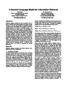
3.2 Recovery of Skill Classication Probabilities Figure 1 shows the relationships between skill classication probabilities for one randomly selected simulated dataset. The plots show the bivariate distribution of classication probabilities of this sample with respect to classication into the mastery level (ak = 1) on skill i and skill j , for skills i, j = 1 . . . 4. 0.2

0.4

0.6

0.8

1.0

0.0

0.2

0.4

0.6

0.8

1.0

0.6

0.8

1.0

0.0

0.6

0.8

1.0

0.0

0.2

0.4

skill1

0.6

0.8

1.0

0.0

0.2

0.4

skill2

0.6

0.8

1.0

0.0

0.2

0.4

skill3

0.0

0.2

0.4

skill4

0.0

0.2

0.4

0.6

0.8

1.0

0.0

0.2

0.4

0.6

0.8

1.0

Figure 1. Plots of skill classication probabilities. In addition to the skill model as given in Equation 5, the 2PL IRT model was estimated for this simulated dataset. Figure 2 shows the relationship between skill mastery probabilities p (transformed to logits, i.e., for probability p, the plot shows log 1−p ) and the overall ability

estimate from the 2PL model. There is an obvious relationship between skill classications and the 2PL parameter for all four skills. Most points in the plots fall into the extremes, so that the examinees classied as masters versus non masters with high probability receive either very high (masters) or very low (nonmasters) 2PL IRT ability estimates. 12

0.5 1.0 1.5

−1.5

−0.5

0.5 1.0 1.5

2PL theta estimate

Skill 3

Skill 4 Skill probability

−1.5

0.0 0.2 0.4 0.6 0.8 1.0

Skill probability −0.5

2PL theta estimate

0.0 0.2 0.4 0.6 0.8 1.0

−1.5

Skill probability

Skill 2

−0.5

0.5 1.0 1.5

0.0 0.2 0.4 0.6 0.8 1.0

Skill probability

0.0 0.2 0.4 0.6 0.8 1.0

Skill 1

−1.5

2PL theta estimate

−0.5

0.5 1.0 1.5

2PL theta estimate

Figure 2. Plots of skill classication probabilities by 2PL ability estimate. Table 4 shows the recovery of skill-pattern probabilities by mdltm using the generating model (i.e., the correctly specied Q-matrix, with parameters estimated by mdltm ). This table contains the true values used for generating the data, the average bias of the estimated skill probabilities, the standard error, and the standardized residual and the RMSE of the estimates as dened above. Table 4 shows that the algorithm recovers the skill pattern probabilities very accurately for the simulated data. This provides some evidence that the mdltm software is capable of recovering the generating parameters of simulated data if the model is specied correctly. The Bonferroni adjusted error level chosen was α = 0.0031 yielding a critical (two-sided) value of zα = 2.955, an interval boundary that none of the residuals in Table 4 exceed. In addition, the homogeneity of bias and RMSE values indicates that the generating probabilities have been reproduced very accurately across skill patterns.

13

Table 4 True Parameters, Bias, S.E, Residual, and RMSE of Skill-Pattern Probabilities Pattern 0000 1000 0100 1100 0010 1010 0110 1110 0001 1001 0101 1101 0011 1011 0111 1111

Truth 0.26041 0.05208 0.05208 0.01041 0.05208 0.01041 0.01041 0.05208 0.05208 0.01041 0.01041 0.05208 0.01041 0.05208 0.05208 0.26041

Bias 0.00030 -0.00050 -0.00071 -0.00011 -0.00009 -0.00011 -0.00016 -0.00020 0.00025 0.00016 0.00036 0.00065 -0.00009 -0.00004 -0.00074 0.00105

s.e. 0.00066 0.00049 0.00063 0.00035 0.00044 0.00031 0.00027 0.00055 0.00056 0.00025 0.00032 0.00052 0.00033 0.00064 0.00060 0.00056

Residual 0.46619 -1.02836 -1.13016 -0.31626 -0.20875 -0.37587 -0.60750 -0.36974 0.44879 0.66666 1.13175 1.23687 -0.30192 -0.06390 -1.24049 1.87895

RMSE 0.00419 0.00315 0.00408 0.00226 0.00283 0.00200 0.00172 0.00351 0.00357 0.00161 0.00209 0.00339 0.00209 0.00405 0.00387 0.00370

3.3 Skill Classication Agreement Table 5 contains a summary of classication accuracy using Cohen's kappa (κ; Cohen, 1960) across the four skills for the rst ve replicates. The values are quite stable, so that the mean was computed for these ve replicates only. The average kappa across the four skills is κ = 0.911, which should be considered a value that indicates almost perfect agreement. Landis & Koch (1977) consider values above 0.6 as indicating substantial agreement, whereas a value above 0.8 is considered indicating almost perfect agreement. Fleiss (1981) considers κ above 0.75 as indicating excellent agreement.

Table 5 Cohen's Kappa, Means, and Standard Deviations for Five Replicates Across the Four Skills Skill 1 2 3 4

Rep 1 0.94027 0.87569 0.87569 0.93541

Rep 2 0.92152 0.87916 0.94375 0.91736

Rep 3 0.92569 0.88125 0.92638 0.90972

Rep 4 0.93472 0.86875 0.92777 0.90694

Rep 5 0.93333 0.87916 0.93402 0.90902 14

Mean 0.93111 0.87680 0.92152 0.91569

St. dev. 0.00746 0.00492 0.02652 0.01170

Table 6 shows the percentage of agreement on the level of skill patterns based on the classication of each simulated response pattern into one of the 24 = 16 possible skill patterns from nonmastery on all four skills to mastery of all four skills, that is,

{(0, 0, 0, 0), (0, 0, 0, 1), . . . , (1, 1, 1, 0), (1, 1, 1, 1)}.

Table 6 Skill Pattern Classication Agreement All four skills correct Three or more correct

1 0.8687 0.9684

2 0.8690 0.9638

3 0.8593 0.9642

4 0.8548 0.9666

5 0.8684 0.9621

For the given skill pattern distribution, the level of chance agreement on all four skill levels is 0.16, compared to a model based agreement on all four skills of about 0.86, so that the model based correct classication is about ve times higher (0.86/0.16 = 5.375) than the classication by chance, given that the base rates (i.e., the true distribution) of the skill-patterns are already known. However, if the distribution of skills is unknown, the all-correct classication by chance drops to 0.0625, which results in a ratio of 13.76 = 0.86/0.0625, so that the all-correct classication hit rate 13.76 times higher than a classication by chance. If classications with three or more correct skill identications are considered, the (three or more) correct rate is about 96.5%.

3.4 Additional Results The appendix (Table A1 and the following tables) contains results of additional simulations using a bifactorial Q-matrix, with four (0/1) skills, 36 items, and 2,880 simulated respondents for each of 40 datasets. In a bifactor-design, one predominant factor (here: skill) is required for all the items; all items may require additional subfactors (skills), which load only on a small subset of items compared to the predominant skill. In the simulation, Skill 1 was the predominant skill; it was required for all 36 items (so that the Q-matrix column for this skill contains only ones, i.e., qi1 = 1 for all i = 1, . . . , 36), whereas Skills 24 are required for dierent item subsets, each comprising approximately one third of the items. The Q-matrix entries for Skill 1 were set to be 1.0 by design, whereas the remaining nonzero entries were randomly assigned for Skills 24. Results are based on analyses with mdltm using 40 datasets simulated using the bifactor design. As was the case for the condition without a predominant skill, most standardized residuals here 15

are also of moderate size (see the appendix). Using a critical zα based on a Bonferroni correction of α shows that a signicant result is obtained based on one residual with a value of −4.05. The RMSE based on 40 simulations are homogeneous and without any obvious outliers. Overall, the simulation parameters for the bifactor Q-matrix data are also recovered very accurately across skill pattern probabilities, slopes, and diculties.2

4. Diagnostic Modeling of TOEFL iBT Data This section presents an analysis of the TOEFL iBT pilot data with the pGDM as introduced above, using dichotomous (0/1) attributes. The TOEFL iBT Reading and the Listening sections of two parallel forms, Form A and Form B, were analyzed by content experts, producing four Q-matrices, one each for Reading Form A, Reading Form B, Listening Form A, and Listening Form B. The TOEFL iBT data contains items with missing responses as well as items scored using a polytomous response format. None of the polytomous or missing responses were recoded (i.e., they were neither collapsed nor assigned to a specic category for the analysis using the mdltm software). All analyses were carried out using a 2.2 GHZ notebook PC and took less than 30 seconds to converge for the larger datasets using the four-skill model. The joint analysis of Reading and Listening using a Q-matrix with eight skills took about 6 minutes.

4.1 Source and Structure of the Data Table 7 gives details on the structure of the TOEFL iBT data that were analyzed with the pGDM. The forms are intended to be parallel; the Reading forms contain 39 and 40 items each and consist of items that are assumed to require the four skills, Word Meaning, Specic Information, Connect Information, and Synthesize & Organize, to very similar degrees. The two Listening Test Forms A and B include 34 items each; the skills that are assumed to be required to answer these items correctly are labeled General Information, Specic Information, Pragmatics & Text Structure, and Inferences & Connections. Tables A4 and A5 in the appendix present the Q-matrices for the four TOEFL iBT datasets that were analyzed here. The analyses were carried out separately for Reading and Listening and separately for both Forms A and B. Most subjects who took Form B also took Form A, so that 379 subjects that took both forms could be matched with respect to their outcomes of the GDM analysis. All four form (A/B) by scale (Reading/Listening) datasets were analyzed both with the 2PL IRT model and the

16

Table 7 Structure of the Language Assessment Pilot Data Used in the Analysis Form Reading

A 39 items

B 40 items

Listening

34 items 2,720

34 items 419

Sample N

Word meaning General information

Skills labels Specic Connect information information Specic information

Pragmatics & text structure

Sythesize & organize Inferences & connections

GDM using the four skills as dened by the expert supplied Q-matrices. Form A was also analyzed jointly, that is, the 39 Reading and the 34 Listening items were analyzed together with a combined Q-matrix of eight skills, as well as with a two-dimensional version of the 2PL IRT model. This was done in order to check whether a joint analysis would provide evidence that Reading and Listening have to be modeled as separate abilities. Form B was not analyzed in this way since the comparably small sample size was deemed insucient for such a high dimensional analysis. Summary results for the joint analysis of Reading and Listening are reported in section 4.3.

4.2 Results and Notes Since the pGDM contains commonly used IRT models like the GPCM as special cases, this allows one to compare IRT results and diagnostic prole scoring results directly with respect to measures of model-data t. Table 8 presents the resulting values for the expected log likelihood per observation (log-penalty) for the dierent models analyzed.

Table 8 Log Likelihood and Log-Penalty for Models Estimated for Reading and Listening Forms A and B Form A A B B

Model 4 Skills GDM 2PL IRT 4 Skills GDM 2PL IRT

Reading -2*LogLike LogPen 116308.06 -21.38 114096.26 -20.97 18517.37 -22.10 18218.45 -21.74

Listening -2*LogLike LogPen 95204.48 -17.50 93125.46 -17.11 14588.96 -17.41 14333.70 -17.10

17

The 2PL model shows uniformly smaller deviance (-2*LogLike) values and consequently smaller absolute log penalties (LogPen) than the four-skill model across the Reading and Listening sections of both test forms. These values indicate that the 2PL model ts the data better than the four-skill model. The number of parameters required is larger for the four-skill model than for the 2PL model, unless the Q-matrix would allow only one nonzero entry for each item (i.e., it would exhibit simple structure). Therefore, information indices like AIC or BIC (Schwarz, 1978) would favor the 2PL, since the number of parameters is smaller and the likelihood is larger for this model. In this sense, the 2PL model may be viewed as the more parsimonious data description. Therefore, the 2PL ability parameters taken from the calibration of the TOEFL iBT data will be used as a benchmark for the classications from the diagnostic model with four skills per subtest and test form. The comparisons to be presented next are organized as follows: First, the skill mastery probabilities are compared to the 2PL ability estimate for Reading and Listening for Test Forms A and B. Second, the correlations of raw scores, IRT ability estimates and ability and skill mastery probabilities will be compared across Test Forms A and B for those examinees who took both Form A and Form B. Then, the joint distributions of skill mastery probabilities across Test Forms A and B will be examined for those examinees who took both Form A and Form B.

4.21 Skill Mastery and Overall Ability, Reading Forms A and B Figure 3 shows the skill mastery probabilities plotted against the overall ability estimate for Reading, Test Forms A and B, for Skills 14. The four plots on the left-hand side show the results for Form A, the four plots on the right-hand side show the results for Form B. It is evident from the plots that Skills 13 are predicted very accurately by the overall 2PL ability estimate. Skill 4 shows an unexpected shape, but there is still a denite relationship to overall ability estimate. The right-hand side of Figure 3 shows the relationship between skill mastery probabilities and overall 2PL ability estimate for Reading, Test Form B. The relationship between skills and ability are very similar to what has been found in Test Form A, except for Skill 4, which seems somewhat less related to overall ability when comparing Form B with Form A. Note that Skill 4 in Reading is special in the sense that Skill 3 is a prerequisite for Skill 4. In Reading Form A, all except one item require Skill 3 whenever Skill 4 is required, whereas several items require only Skill 3 (and maybe some other skill), but not Skill 4. In Form B, all items that require Skill 4 also require Skill 3. 18

0.5

1.0

1.5

−0.5 0.0

0.5

1.0

1.5

0.6 0.4

Skill probability

0.2 0.0

0.0 −1.5

−1.5

−0.5 0.0

0.5

1.0

1.5

−1.5

−0.5 0.0

0.5

2PL theta estimate

Skill 1 Form B

Skill 2 Form B

Skill 3 Form B

Skill 4 Form B

1.0

0.5

1.0

1.5

−0.5 0.0

0.5

1.0

1.5

1.0

1.5

0.6 0.4

Skill probability

0.2 0.0

0.0 −1.5

1.5

0.8

0.8 0.2

0.4

0.6

Skill probability

0.6 0.0

0.2

0.4

Skill probability

0.8

0.8 0.6 0.4 0.2

−0.5 0.0

2PL theta estimate

1.0

1.0

2PL theta estimate

1.0

2PL theta estimate

0.0 −1.5

0.8

1.0 0.2

0.4

0.6

Skill probability

0.8

1.0 0.6 0.0

0.2

0.4

Skill probability

0.8

0.8 0.6 0.4

Skill probability

0.2 0.0

−0.5 0.0

Skill 4 Form A

2PL theta estimate

1.0

−1.5

Skill probability

Skill 3 Form A 1.0

Skill 2 Form A

1.0

Skill 1 Form A

−1.5

2PL theta estimate

−0.5 0.0

0.5

1.0

1.5

−1.5

2PL theta estimate

−0.5 0.0

0.5

2PL theta estimate

Figure 3. Skill mastery and reading ability.

Note. For Form A, N=2,720, and for Form B, N=420.

4.22 Skill Mastery and Overall Ability, Listening Forms A and B A more homogenous relation to the 2PL ability estimate is found for the Listening subscales. Figure 4 shows the plots of skill mastery probabilities and overall 2PL ability estimate for test Form A and Form B. The top line graphs show the results for Form A, and the bottom graphs show results for Form B. All skill mastery probabilities are highly related to overall 2PL ability, where the width of the resulting shape depends mainly on how many items per skill are available. The four skill probabilities are related to the overall 2PL ability in very similar ways for both test forms. The Pearson correlation would be misleading to report for the kind of curvilinear relationship observed in the above plots. An appropriate transformation of the skill mastery probabilities is to calculate the logit

l = log

p 1−p

for each examinee. This transforms the bounded classication probability p to a value l that is unbounded much like the 2PL ability estimate θ, which makes a linear relationship between l and θ a reasonable assumption. The correlations found for these transformed skill classication probabilities with the overall 2PL ability estimate range between 0.8 to 0.95, for Reading Skills 13, Form A. Correlations are somewhat lower for Skill 4 (see Table 9). This indicates that most of the

19

1.0

1.5

−0.5 0.0

0.5

1.0

1.5

0.2

0.4

Skill probability

0.6

0.8

1.0 −1.5

0.0 −1.5

−0.5 0.0

0.5

1.0

1.5

−1.5

−0.5 0.0

0.5

2PL theta estimate

2PL theta estimate

Skill 1 Form B

Skill 2 Form B

Skill 3 Form B

Skill 4 Form B

0.5

1.0

1.5

−0.5 0.0

0.5

1.0

1.5

1.5

0.6 0.4

Skill probability

0.0 −1.5

2PL theta estimate

1.0

0.2

0.2 0.0 −1.5

1.5

0.8

1.0 0.6 0.4

Skill probability

0.8

1.0 0.6 0.0

0.2

0.4

Skill probability

0.8

0.8 0.6 0.4 0.2

−0.5 0.0

2PL theta estimate

1.0

1.0

2PL theta estimate

0.0 −1.5

0.6 0.2 0.0

0.0 0.5

0.4

Skill probability

0.8

1.0 0.6 0.2

0.4

Skill probability

0.8

0.8 0.6 0.4

Skill probability

0.2 0.0

−0.5 0.0

Skill 4 Form A

2PL theta estimate

1.0

−1.5

Skill probability

Skill 3 Form A 1.0

Skill 2 Form A

1.0

Skill 1 Form A

−0.5 0.0

0.5

2PL theta estimate

1.0

1.5

−1.5

−0.5 0.0

0.5

2PL theta estimate

Figure 4. Skill mastery probabilities and overall ability, Listening Forms A and B. variance can be picked up by the overall 2PL ability estimate (denoted by ThetaRA or ThetaLA in the table), for all four skills in the case of the Listening subscale and for three out of four for the Reading skills.

Table 9 Correlations Between Logit Skill Probabilities and the Overall 2Pl Ability Estimate, Reading Form A ThetaRA Skill1RA Skill2RA Skill3RA

Skill1RA 0.8541

Skill2RA 0.8929 0.7980

Skill3RA 0.9500 0.8102 0.8652

Skill4RA 0.4549 0.4285 0.4770 0.4209

Table 10 shows the correlations between the logit skill probabilities (denoted by Skill1LA to Skill4LA) and the overall ability estimate (ThetaLA) of the Listening skills for Form A; the correlations for Form B are similar (compare Figure 4) and are not presented due to space constraints. The correlations are all between 0.85 and 0.96, so that it may be conjectured that all the variables tabulated in the gure below are interchangeable measures of the same underlying variable.

20

Table 10 Correlations Between Logit Skill Probabilities and the Overall 2Pl Ability Estimate, Listening Form A ThetaLA Skill1LA Skill2LA Skill3LA

Skill1LA 0.9498

Skill2LA 0.9659 0.9313

Skill3LA 0.9252 0.9230 0.8848

Skill4LA 0.8977 0.9112 0.8836 0.8556

4.23 Relationships Between Forms A and B The correlation between relative raw score (score/max score) and the overall 2PL ability estimate for Reading across Forms A and B, obviously only based on examinees who took both forms, is around 0.8. The same holds for the Listening subscale. Figure 5 shows the scatterplots illustrating this relationship. It can be seen that the relative raw score has only a limited number of possible values and the data points are located on a grid of possible coordinates, since the relative raw score, being a simple transform of the raw score, is a discrete random variable. The 2PL/GPCM based ability estimates are slightly more spread out and do not show the grid eect observed for the proportion correct, since the sucient statistic for the ability estimates is a weighted sum of item scores. Theta, A vs. B, Reading

0.2

−1

Form B Reading 0.4 0.6 0.8

Form B Reading 0 1 2

1.0

Raw Scores, A vs. B, Reading

0.2

0.4 0.6 0.8 Form A Reading

1.0

−1.0

2.0

Theta, A vs. B, Listening

Form B Listening −2 −1 0 1

Form B Listening 0.2 0.4 0.6 0.8 1.0

2

Raw Scores, A vs. B, Listening

0.0 1.0 Form A Reading

0.2

0.4 0.6 0.8 Form A Listening

1.0

−1.5

−0.5 0.5 Form A Listening

1.5

Figure 5. Relationship between overall estimates for Forms A and B for Reading and Listening skills.

21

Table 11 shows the intercorrelations for logit skill probabilities and 2PL ability estimates for Reading across Form A and Form B. The 2PL ability estimate of Forms A and B correlate to 0.81, which is very close to the logit skill probability correlations for the Reading Skills 13. Again, Skill 4 on Form A shows somewhat lower correlations with the other skills and the 2PL ability. Remember that Skill 4 on Form B does not have any items where Skill 3 is not required. This skill shows even negative correlations with the other variables in the table.

Table 11 Correlation Between Reading Logit Skill Probabilities and 2PL Ability for Forms A and B ThetaRB Skill1RB Skill2RB Skill3RB Skill4RB

ThetaRA 0.81644 0.77173 0.78690 0.81318 -0.09303

Skill1RA 0.71986 0.73583 0.72275 0.73856 -0.10294

Skill2RA 0.72834 0.71120 0.73241 0.74024 -0.16095

Skill3RA 0.78031 0.74149 0.77894 0.78791 -0.14863

Skill4RA 0.34320 0.35930 0.37202 0.35408 0.04358

The correlations between the Listening skills and the Listening 2PL ability estimates are presented in Table 12. The range of correlations is more homogenous than for Reading, a result to be expected based on the plots shown previously.

Table 12 Correlation Between Listening Logit Skill Probabilities and 2PL Ability for Forms A and B ThetaLB Skill1LB Skill2LB Skill3LB Skill4LB

ThetaLA 0.79550 0.76390 0.77349 0.76147 0.74249

Skill1LA 0.76447 0.75653 0.75986 0.73816 0.72383

Skill2LA 0.76993 0.74784 0.76290 0.74804 0.71791

Skill3LA 0.75026 0.72795 0.73089 0.72905 0.71729

Skill4LA 0.71276 0.70831 0.70027 0.69545 0.67395

The correlation across forms are also somewhat more homogenous for Listening. The correlations range between 0.67 (Listening, Skill 4, Form A and Listening, Skill 4, Form B) and 0.79 (Listening, Skill 1, Form A and Listening, Skill 1, Form B).

22

4.24 Skill Mastery Probabilities Across Test Forms Figure 6 shows the skill mastery probabilities for Reading across Test Forms A and B for those 379 individuals who took both test forms. Recall that Skill 4 had a funny S-shape in both test forms whereas Skills 13 were monotonically related to the overall Reading 2PL ability estimate.

0.2

0.4

0.6

0.8

0.0 0.2 0.4 0.6 0.8 1.0

Form B 0.0

1.0

0.0

0.2

0.4

0.6

0.8

1.0

Form A

Form A

Skill 3, A vs. B, Reading

Skill 4, A vs. B, Reading

Form B

0.0 0.2 0.4 0.6 0.8 1.0

Form B

Skill 2, A vs. B, Reading

0.0

0.2

0.4

0.6

0.8

1.0

0.0 0.2 0.4 0.6 0.8 1.0

Form B

0.0 0.2 0.4 0.6 0.8 1.0

Skill 1, A vs. B, Reading

0.0

0.2

Form A

0.4

0.6

0.8

1.0

Form A

Figure 6. Skill probabilities for Reading Across Form A and Form B. There is an obvious pattern in the plots for Skills 13. The majority of points cluster around the skill coordinates (0,0) and (1,1). This can be seen as a sign of consistency in classications of the mastery of skills. Recall that the logits of the values depicted in the plots correlate about 0.8 for Reading Skills 13. On the other hand, there are also a few examinees who have a mastery probability of greater than 0.5 for Form A and a probability below 0.5 for Form B, and vice-versa. These are the observations that would be classied as masters based on their mastery probability one test form and as nonmasters according to their mastery probability on the other test form.3 Skill 4 stands out from the others, lacking the observed pattern of noticeable agreement between the skill mastery probabilities. This skill probability variable was also functioning dierently with respect to the overall ability estimate. The consistency across forms is much lower for Skill 4, and there is no noticeable clustering around the (0,0) and (1,1) coordinates, indicating a lack of agreement on Skill 4 between the two test forms. Figure 7 shows the same comparison plots for the Listening skills across Form A and Form 23

B. Recall that all the Listening skills had shown a strict monotone relationship with the overall Listening 2PL ability estimate in both test forms.

0.2

0.4

0.6

0.8

0.0 0.2 0.4 0.6 0.8 1.0

Form B 0.0

1.0

0.0

0.2

0.4

0.6

0.8

1.0

Form A

Form A

Skill 3, A vs. B, Listening

Skill 4, A vs. B, Listening

Form B

0.0 0.2 0.4 0.6 0.8 1.0

Form B

Skill 2, A vs. B, Listening

0.0

0.2

0.4

0.6

0.8

1.0

0.0 0.2 0.4 0.6 0.8 1.0

Form B

0.0 0.2 0.4 0.6 0.8 1.0

Skill 1, A vs. B, Listening

0.0

Form A

0.2

0.4

0.6

0.8

1.0

Form A

Figure 7. Skill probabilities for Listening across Test Forms A and B. As was the case for Reading Skills 13, the plots for the Listening Skills 14 show clustering around the coordinates (0,0) and (1,1). This indicates that most individuals would be classied as either master or nonmaster in the same way by both test forms. Note however, that for Listening, the plots show a slight asymmetry; there seems to be a few more individuals who receive a higher than 0.5 mastery classication probability for test Form B with a probability of mastery close to 0.0 for Form A than the other way around. In the plots, it may seem as if the lower right corner of each plot to contain a little fewer observations than the upper left corner. This may be an artifact of the relatively small sample employed; it cannot be decided from these plots alone.

4.3 Combined Analysis of Reading and Listening Since the logit transformed skill probabilities for Reading and Listening correlate very highly with the corresponding 2PL ability estimate, some additional analyses were carried out in order to check whether the 2PL model would suce to describe the combined data for Reading and Listening adequately. Table 8 shows the log-likelihoods for the dierent models estimated for the combined Reading and Listening data. In order to investigate whether these conclusions 24

hold up even if the Reading and Listening are analyzed jointly, additional analyses with an eight-dimensional skill model, a two-dimensional conrmatory 2PL model, and a unidimensional 2PL model across the combined Reading and Listening items were carried out. Table 13 shows the deviance and log penalty values for the joint analyses of Reading and Listening subscales for Form A. Test Form B was not analyzed jointly for Reading and Listening, since the small sample for this form was deemed too small to support a joint model for 74 items.

Table 13 Joint Analysis Results for Reading and Listening Form A Model 8 Skills GDM 2-D 2PL IRT 1-D 2PL IRT

-2*LogLik 195437.39 191013.36 191650.13

LogPen -35.93 -35.11 -35.23

The deviance, and consequently the absolute log penalty, is smallest for the two-dimensional 2PL (2-D 2PL) model in the joint analysis of Reading and Listening. The eight-skill model has the largest deviance and absolute log penalties, indicating a slightly poorer t than the model data t of the 2PL model and 2-D 2PL. Given that the eight-skill model shows the largest deviance of the models estimated here, and given that the eight-skill model requires more parameters than each of the 2PL models, it may be concluded that the 2PL models are preferable in terms of model-data t and parsimony. Using the combined 2PL model may be advised in order to increase the accuracy of parameter estimates and in order to facilitate the study of correlations between Reading and Listening for dierent test forms on the latent variable level.

5. Conclusions The goal of the work presented here is to present the applicability of the GDM and its estimation when making use of standard maximum likelihood techniques. The results of the simulation study show that the pGDM is capable of recovering parameters data very accurately here, even if no information about the true parameter values is used in estimation. The simulation used data similar to the data structures from the TOEFL iBT pilot study. Results show that the estimated skill pattern probabilities as well as estimates of slope and diculty parameters are very close to the generating parameters. This statement holds for both, the bifactor data, where one

25

predominant skill was present in all items, as well as for the more balanced condition, where each skill was present in about 50% of the items. Additional studies are necessary in order to be able to generalize these ndings to smaller and larger sample sizes, as well as additional variables that have an impact on the latent structures that represent the skill space, such as the number of skills and the granular levels of the skills. For the combined Reading and Listening real data from the TOEFL iBT pilot, an IRT model with a two-dimensional 2PL ability, one ability each for Reading and for Listening, t the data slightly better than a undimensional 2PL model with one common ability holding across Reading and Listening. When looking at the Reading and Listening data separately, the four-skill models for Reading and for Listening with the TOEFL iBT pilot data t less well than the 2PL models for these subscales. For both test forms, the four Listening skills are highly correlated, as are Reading Skills 13. The Reading subscale includes one skill (Skill 4) that diers from the general pattern in that it correlates lower than the other skills among each other and it shows the lowest correlations across Forms A and B. The pGDM was estimated for 4+1 (four separate and one combined analysis) dierent real datasets from the TOEFL iBT pilot study. The analyses successfully showed similarities between the skills across test forms, even though the Q-matrices were retrotted to an existing test. Results from comparing the skill model with the 2PL may provide insight for test development in the sense that some skills may need clearer separation by making use of specically engineered items, if a skill model is to be used. In the current form, the 2PL ts the observed data a little better than a model with four mastery/nonmastery skills. This is an area where additional research on revisions that might be made to the Q-matrix, as well as on future modications to the test, may prove useful. The Reading Skill 4 assessed in Form B shows very low correlations with all other variables in the study, even with Reading Skill 4 in Form A. Some additional analysis of the Reading test items may allow one to improve on the Q-matrix in the sense that more separable skills may be dened in a revised version. The output from the mdltm software used for estimating the 4-Skill and the 2PL models contains item t information that may provide additional information for revisions of the test and maybe changes to the Q-matrices. This additional information can come from the diagnostics available through estimating the pGDM and from presenting the outcomes in plots like the ones shown in Figure 7. The 2PL IRT model used in the analysis is not analyzed any further in this report, more 26

specically, the 2PL model was not tested against the 3PL4 , since the focus of this report is on diagnostic models. The analyses showed that a comparably better model-data t can be achieved using the 2PL model, and that the four-skill model, if it is applied, results in highly correlated skills for the TOEFL iBT data. If skill classications and skill prole reports to clients are required for TOEFL iBT Reading and Listening, these reports should be accompanied by a note pointing out the high correlations among the skills and the eects these high correlations will have on the reports. The majority, or seven out of eight Reading and Listening skills, are strongly related to overall ability, and the eighth skill is found not to correlate across test forms in the pilot data. For the current form of the TOEFL iBT instrument and the current Q-matrices, the skill prole reports would include four highly correlated skill classications for the Listening section, and three highly correlated skill classications for the Reading section. If highly correlated skills were to be reported, most skill patterns would be (0,0,0,0)that is, a lack of mastery on all skillsor (1,1,1,1)that is, mastery on all skills. This is caused by reducing the available information (the skill mastery probability is dichotomized using some cut point) to a 0/1 mastery/nonmastery variable. On the other hand, if a single IRT-based ability estimate were to be made available for every examinee, the ability estimate could be accompanied by a measure of uncertainty or by a descriptive prociency level that states in qualitative terms what a student at or above this level is able to do.

27

References Almond, R. G., & Mislevy, R.J. (1999). Graphical models and computerized adaptive testing.

Applied Psychological Measurement, 23, 223-237. Birnbaum, A. (1968). Some latent trait models. In F. M. Lord & M. R. Novick (Eds.), Statistical

theories of mental test scores. Reading, MA: Addison-Wesley. Cohen, J. (1960). A coecient of agreement for nominal scales. Educational and Psychological

Measurement, 20, 37-46. Davier, M. von, (2001). WINMIRA 2001: A software for estimating Rasch models, mixed and HYBRID Rasch models, and the latent class analysis [Computer software]. Retrieved August 5, 2005, from the Assessment System Corporation: http://www.assess.com/Software/WINMIRA.htm. Davier, M., von, & Yamamoto, K. (2004a, October). A class of models for cognitive diagnosis. Paper presented at the 4th Spearman Conference, Philadelphia, PA. Davier,M., von, & Yamamoto, K. (2004b, December). A class of models for cognitive diagnosis -

and some notes on estimation. Paper presented at the ETS Tucker Workshop Seminar, Princeton, NJ. Davier, M., von, & Yamamoto, K. (2004c). Partially observed mixtures of IRT models: An extension of the generalized partial credit model. Applied Psychological Measurement, 28, 389-406. de la Torre, J., & Douglas, J. A. (2004). Higher order latent trait models for cognitive diagnosis.

Psychometrika, 69(3), 333-353. DiBello, L., Stout, W., & Roussos, L. (1995). Unied cognitive/psychometric diagnostic assessment likelihood-based classication techniques. In P. Nichols, S. Chipman, & R. Brennan (Eds.), Cognitively diagnostic assessment (pp. 361-389). Hillsdale , NJ: Erlbaum. Fleiss, J. (1981). Statistical methods for rates and proportions. New York: John Wiley & Sons. Formann, A. K. (1985). "Constrained Latent Class Models: Theory and Applications," British

Journal of Mathematical and Statistical Psychology, 38, 87-111. Haberman S. J. (1979). Qualitative data analysis: Vol. 2. New developments. New York: Academic Press. Haertel, E. H. (1989). Using restricted latent class models to map the skill structure of achievement items. Journal of Educational Measurement. 26(4), 301-321. 28

Hagenaars, J. A. (1993). Loglinear models with latent variables. Newbury Park, CA: Sage. Hartz, S., Roussos, L., & Stout, W. (2002). Skills diagnosis: Theory and Practice. User Manual for Arpeggio software [Computer software manual]. Princeton, NJ: ETS. Landis, J., & Koch, G. (1977). The measurement of observer agreement for categorical data.

Biometrics, 33, 159-174. Lazarsfeld, P. F., & Henry N. W. (1968). Latent structure analysis. Boston: Houghton Miin. Linacre, J. M. (1989). Many-facet Rasch measurement. Chicago: MESA Press. Maris, E. (1999). Estimating multiple classication latent class models. Psychometrika, 64(2), 187-212. Muraki, E. (1992). A generalized partial credit model: Application of an EM algorithm. Applied

Psychological Measurement, 16(2), 159-176. Rasch, G. (1960). Probabilistic models for some intelligence and attainment tests. Chicago: University of Chicago Press. Tatsuoka, K. K. (1983). Rule space: An approach for dealing with misconceptions based on item response theory. Journal of Educational Measurement, 20, 345-54.

29

Notes 1

Assuming xed skill levels al on the remaining skills l 6= k and a slope parameter γik > 0.

2

Additional simulations were carried out using the bifactor design as well as a random Q-matrix

with a uniform skill pattern distribution. The results of these analyses are not reported here, since the recovery was equally good under the uniform skill probabilities conditions as it was under the conditions presented here. 3

Unless a region of indierence is used, which acknowledges that there is insucient information

for some examinees falling into this region to classify these with high condence. 4

The item t measures available in mdltm were examined informally in search for indications of

model mist, but no obvious evidence of item mist or evidence to indicate a need to modeling guessing behavior was found.

30

Appendix Parameter Recovery in the Bifactorial Design Table A1 Skill Pattern Probabilities Recovery, Bifactorial Q-Matrix Pattern 0000 1000 0100 1100 0010 1010 0110 1110 0001 1001 0101 1101 0011 1011 0111 1111

Truth 0.26041 0.05208 0.05208 0.01041 0.05208 0.01041 0.01041 0.05208 0.05208 0.01041 0.01041 0.05208 0.01041 0.05208 0.05208 0.26041

Bias 0.00155 -0.00042 -0.00056 -0.00007 0.00129 -0.00009 -0.00002 -0.00152 -0.00188 0.00050 -0.00012 0.00071 0.00001 0.00055 -0.00029 0.00038

s.e. 0.00116 0.00051 0.00052 0.00037 0.00092 0.00043 0.00036 0.00087 0.00096 0.00039 0.00044 0.00065 0.00037 0.00074 0.00038 0.00091

31

Residual 1.33330 -0.82776 -1.07887 -0.19135 1.39044 -0.22715 -0.07836 -1.74485 -1.94640 1.28892 -0.28609 1.08053 0.01711 0.75304 -0.76943 0.42199

RMSE 0.00753 0.00327 0.00333 0.00235 0.00601 0.00276 0.00229 0.00571 0.00639 0.00252 0.00282 0.00423 0.00234 0.00472 0.00246 0.00577

Table A2 True Parameters and RMSE for the Bifactorial Simulated Data True parameters

RSME

Item

γ1i

γ2i

γ3i

γ4i

βi

Item

γ1i

γ2i

γ3i

γ4i

βi

1

0.84480

-/-

1.41411

2

0.83363

-/-

0.96008

0.73681

-1.07045

1

0.08024

-/-

0.09455

0.09728

0.07978

-/-

-0.13508

2

0.05202

-/-

0.05728

-/-

0.04860

3

1.01036

-/-

-/-

4

0.87668

-/-

0.74088

-/-

-0.28843

3

0.04268

-/-

-/-

-/-

0.04078

-/-

-0.87271

4

0.04978

-/-

0.06219

-/-

5

1.05087

-/-

-/-

0.05643

-/-

0.71664

5

0.04619

-/-

-/-

-/-

0.04710

6

0.93369

1.06729

7

0.95873

0.87190

1.33901

-/-

-0.22105

6

0.05816

0.08130

0.07683

-/-

0.09998

-/-

-/-

0.91743

7

0.06184

0.05423

-/-

-/-

0.05323

8

1.24306

1.36422

-/-

9

1.37841

-/-

0.89835

-/-

1.66109

8

0.09192

0.08303

-/-

-/-

0.08891

1.26263

0.19979

9

0.07916

-/-

0.08413

0.08161

0.06201

10

1.01483

-/-

-/-

-/-

0.31113

10

0.04500

-/-

-/-

-/-

0.04848

11

1.35033

1.23710

12

0.95370

0.96446

-/-

-/-

1.12534

11

0.06837

0.08584

-/-

-/-

0.06099

-/-

1.20726

0.58774

12

0.07396

0.08987

-/-

0.09001

0.07387

13

1.10869

-/-

-/-

14

0.80219

-/-

-/-

-/-

1.23987

13

0.05488

-/-

-/-

-/-

0.05452

0.96845

0.13247

14

0.06204

-/-

-/-

0.05504

15

1.06310

-/-

-/-

0.05088

-/-

1.53576

15

0.06737

-/-

-/-

-/-

0.05828

16

1.48846

1.02788

17

1.10993

0.92498

1.05185

-/-

-0.11062

16

0.08574

0.09944

0.10185

-/-

0.06538

0.67771

-/-

0.78302

17

0.05015

0.06302

0.07042

-/-

18

0.99415

0.06761

1.00850

-/-

-/-

0.10392

18

0.04048

0.04621

-/-

-/-

0.04800

19 20

0.83384

-/-

0.60012

-/-

0.57051

19

0.05277

-/-

0.06334

-/-

0.05085

1.24928

0.65850

-/-

-/-

0.57814

20

0.05689

0.05717

-/-

-/-

0.04269

21

0.72484

1.00393

-/-

-/-

0.62558

21

0.06176

0.06470

-/-

-/-

0.05370

22

0.93377

-/-

0.56017

-/-

-0.73747

22

0.06095

-/-

0.06121

-/-

0.05036

23

1.19618

0.91164

0.65791

-/-

-0.77870

23

0.08016

0.07075

0.07365

-/-

0.07541

24

1.43815

-/-

1.04525

-/-

1.61808

24

0.10487

-/-

0.08851

-/-

0.09544

25

1.00610

-/-

-/-

-/-

-0.65119

25

0.03969

-/-

-/-

-/-

0.04543

26

0.84289

0.91225

-/-

-/-

1.10440

26

0.06224

0.06989

-/-

-/-

0.05531

27

1.06508

-/-

-/-

0.90190

0.06197

27

0.05776

-/-

-/-

0.06623

0.04705

28

0.82383

0.91012

-/-

0.90019

0.20377

28

0.06601

0.06591

-/-

0.07335

0.05886

29

1.04186

1.00876

-/-

-/-

0.32691

29

0.05778

0.06918

-/-

-/-

0.05120

30

1.03020

-/-

-/-

0.99946

-0.76692

30

0.07211

-/-

-/-

0.06652

0.06011

31

0.93130

-/-

-/-

-/-

-1.23301

31

0.04410

-/-

-/-

-/-

0.04356

32

1.18117

-/-

1.01277

1.07144

-1.01561

32

0.08372

-/-

0.08958

0.07584

0.08614

33

1.18379

-/-

-/-

1.19949

-0.93439

33

0.07149

-/-

-/-

0.07626

0.08624

34

0.88880

-/-

-/-

-/-

-3.61158

34

0.14570

-/-

-/-

-/-

0.16567

35

1.11204

1.18414

-/-

-/-

-1.47219

35

0.06431

0.07213

-/-

-/-

0.08081

36

0.64151

-/-

0.94236

-/-

-0.50421

36

0.05332

-/-

0.07415

-/-

0.05411

32

Table A3 Mean Bias and Standardized Residuals for the Bifactor Data Mean bias

Standardized residuals

Item

γ1i

γ2i

γ3i

γ4i

βi

item

γ1i

1

-0.00776

-/-

-0.00688

0.01139

-0.00515

1

-0.60711

2

0.00597

-/-

-0.00462

-/-

0.01225

2

0.72181

3

0.00285

-/-

-/-

-/-

-0.01500

3

0.41844

4

0.00514

-/-

0.00237

-/-

-0.01538

4

0.64836

5

-0.00646

-/-

-/-

-/-

-0.00715

5

6

-0.00102

0.01349

-0.00752

-/-

0.00274

7

-0.00912

0.00360

-/-

-/-

0.01154

8

0.01389

0.00305

-/-

-/-

0.01021

9

-0.00438

-/-

0.00308

0.00475

-0.00091

10

0.01054

-/-

-/-

-/-

11

-0.00140

0.02099

-/-

12

-0.00298

-0.01097

-/-

13

-0.00011

-/-

-/-

14

-0.01529

-/-

-/-

15

0.00232

-/-

-/-

16

0.03241

-0.01192

17

0.01125

0.00479

18

-0.00427

-0.00984

γ2i

γ3i

γ4i

βi

-/-

-0.45620

0.73647

-0.40428

-/-

-0.50605

-/-

1.62753

-/-

-/-

-/-

-2.47030

-/-

0.23873

-/-

-1.76881

-0.88257

-/-

-/-

-/-

-0.96029

6

-0.11028

1.05105

-0.61421

-/-

0.17177

7

-0.93149

0.41632

-/-

-/-

1.38670

8

0.95470

0.23006

-/-

-/-

0.72206

9

-0.34677

-/-

0.22904

0.36413

-0.09232

0.01285

10

1.50587

-/-

-/-

-/-

1.71672

-/-

-0.00429

11

-0.12879

1.57519

-/-

-/-

-0.44118

-0.00180

0.01269

12

-0.25251

-0.76803

-/-

-0.12517

1.08939

-/-

0.00476

13

-0.01297

-/-

-/-

-/-

0.54748

0.00051

0.01103

14

-1.58829

-/-

-/-

0.05791

1.38679

-/-

0.01221

15

0.21531

-/-

-/-

-/-

1.33896

0.00692

-/-

0.00823

16

2.55051

-0.75449

0.42583

-/-

0.79311

-0.01074

-/-

0.00029

17

1.43867

0.47609

-0.96440

-/-

0.02757

-/-

-/-

0.01437

18

-0.66287

-1.36091

-/-

-/-

1.96074

19

0.01408

-/-

-0.01316

-/-

0.00704

19

1.72980

-/-

-1.32653

-/-

0.87301

20

-0.00152

0.00892

-/-

-/-

-0.00163

20

-0.16691

0.98743

-/-

-/-

-0.23873

21

-0.01391

0.01637

-/-

-/-

-0.00105

21

-1.44395

1.63338

-/-

-/-

-0.12287

22

0.00899

-/-

-0.00014

-/-

0.00929

22

0.93151

-/-

-0.01459

-/-

1.17263

23

-0.01364

0.02515

-0.00548

-/-

-0.00307

23

-1.07857

2.37516

-0.46661

-/-

-0.25469

24

0.03524

-/-

0.02412

-/-

0.02620

24

2.22840

-/-

1.76874

-/-

1.78313

25

-0.00409

-/-

-/-

-/-

0.01159

25

-0.64767

-/-

-/-

-/-

1.64883

26

-0.01229

0.01175

-/-

-/-

0.00817

26

-1.25809

1.06499

-/-

-/-

0.93288

27

-0.00778

-/-

-/-

0.00720

0.00300

27

-0.84982

-/-

-/-

0.68314

0.39936

28

-0.02855

-0.00240

-/-

0.02343

0.00955

28

-2.99681

-0.22817

-/-

2.10567

1.02748

29

-0.01497

0.01545

-/-

-/-

-0.00351

29

-1.67514

1.43164

-/-

-/-

-0.43009

30

-0.01994

-/-

-/-

0.00317

0.00116

30

-1.79750

-/-

-/-

0.29830

0.12053

31

0.00180

-/-

-/-

-/-

0.00825

31

0.25577

-/-

-/-

-/-

1.20461

32

-0.01353

-/-

0.00606

-0.00201

-0.00832

32

-1.02307

-/-

0.42390

-0.16564

-0.60600

33

-0.02533

-/-

-/-

-0.02981

0.00828

33

-2.36692

-/-

-/-

-2.65322

0.60248

34

0.03201

-/-

-/-

-/-

-0.03840

34

1.40661

-/-

-/-

-/-

-1.48826

35

0.00739

0.00260

-/-

-/-

-0.00601

35

0.72247

0.22603

-/-

-/-

-0.46644

36

0.00610

-/-

0.00212

-/-

0.00213

36

0.72017

-/-

0.17933

-/-

0.24700

33

Q-Matrices Used for the TOEFL iBT Data Table A4 TOEFL iBT Field Test Q-Matrix, Listening Forms Form

General

Specic

Pragmatics &

Inferences &

Form

General

Specic

Pragmatics &

Inferences &

A

information

information

text struct

connections

B

information

information

text struct

connections

1

1

0

0

0

1

1

0

0

0

2

0

1

0

0

2

0

0

1

1

3

0

1

0

0

3

0

1

0

0

4

0

1

0

0

4

0

0

1

0

5

0

0

1

0

5

0

0

0

1

6

1

0

0

0

6

1

0

0

0

7

0

1

0

0

7

0

1

0

1

8

0

1

0

0

8

0

1

0

0

9

0

0

1

0

9

0

1

0

0

10

0

0

1

1

10

0

0

1

0

11

1

0

0

1

11

1

0

0

0

12

0

0

1

1

12

0

0

1

0

13

0

0

0

1

13

0

1

0

0

14

0

1

0

0

14

0

0

0

1

15

0

0

1

1

15

0

1

0

0

16

0

0

1

0

16

0

0

1

0

17

1

0

0

1

17

1

0

0

0

18

0

1

0

0

18

0

0

1

0

19

0

1

0

0

19

0

1

0

0

20

0

1

0

1

20

0

1

0

0

21

0

1

0

0

21

0

0

1

0

22

0

0

1

0

22

0

0

1

0

23

0

1

0

0

23

1

0

0

0

24

0

0

1

1

24

0

1

0

1

25

0

1

0

0

25

0

0

1

0

26

0

1

0

0

26

0

1

0

0

27

0

1

0

0

27

0

0

1

0

28

0

0

1

0

28

0

0

1

0

29

1

0

0

1

29

1

0

0

0

30

0

0

0

1

30

0

0

1

0

31

0

1

0

0

31

0

1

0

0

32

0

1

0

1

32

0

0

0

1

33

0

0

1

1

33

0

0

1

0

34

0

0

1

0

34

0

0

1

0

34

Table A5 TOEFL iBT Field Test Q-Matrix, Reading Forms Form

Word

Specic

Connect

Synthesize

Form

Word

Specic

Connect

Synthesize

A

meaning

information

information

& organize

B

meaning

information

information

& organize

1

1

0

0

0

1

1

0

0

0

2

0

0

1

0

2

0

1

0

0

3

1

0

0

0

3

0

0

1

1

4

0

1

0

0

4

0

0

1

1

5

0

0

1

1

5

1

0

0

0

6

1

0

0

0

6

0

1

0

0

7

0

1

0

0

7

1

0

0

0

8

1

0

1

1

8

0

0

1

0

9

0

0

1

0

9

0

1

0

0

10

0

0

1

1

10

0

1

0

0

11

0

0

1

0

11

0

0

1

0

12

0

0

1

1

12

0

0

1

1

13

0

1

0

0

13

0

1

0

0

14

0

1

0

0

14

1

0

0

0

15

0

1

1

0

15

0

1

0

0

16

1

0

0

0

16

0

0

1

1

17

0

0

1

0

17

0

0

1

0

18

1

0

0

0

18

1

0

0

0

19

0

0

1

0

19

0

0

1

0

20

1

0

0

0

20

1

0

0

0

21

0

0

1

0

21

0

0

1

0

22

0

0

1

0

22

0

0

1

0

23

0

1

0

1

23

1

0

1

0

24

0

0

1

1

24

0

1

0

0

25

0

0

1

0

25

0

0

1

0

26

0

0

1

1

26

0

0

1

1

27

0

1

0

0

27

0

1

0

0

28

1

1

0

0

28

1

0

0

0

29

1

0

0

0

29

0

0

1

0

30

0

1

0

0

30

0

0

1

0

31

0

0

1

0

31

0

1

0

0

32

1

0

0

0

32

0

1

0

0

33

0

1

0

0

33

1

1

0

0

34

0

0

1

1

34

0

1

0

0

35

0

1

0

0

35

0

0

1

1

36

0

1

1

0

36

1

0

0

0

37

1

0

0

0

37

1

0

0

0

38

0

0

1

0

38

0

0

1

1

39

0

0

1

1

39

0

0

1

0

.

.

.

.

.

40

0

0

1

1

35