JOURNAL OF CHEMICAL PHYSICS
VOLUME 121, NUMBER 8
22 AUGUST 2004
A general diagrammatic algorithm for contraction and subsequent simplification of second-quantized expressions Arteum D. Bochevarova) and C. David Sherrillb) School of Chemistry and Biochemistry, Georgia Institute of Technology, Atlanta, Georgia 30332-0400
共Received 3 May 2004; accepted 28 May 2004兲 We present a general computer algorithm to contract an arbitrary number of second-quantized expressions and simplify the obtained analytical result. The functions that perform these operations are a part of the program Nostromo which facilitates the handling and analysis of the complicated mathematical formulas which are often encountered in modern quantum-chemical models. In contrast to existing codes of this kind, Nostromo is based solely on the Goldstone-diagrammatic representation of algebraic expressions in Fock space and has capabilities to work with operators as well as scalars. Each Goldstone diagram is internally represented by a line of text which is easy to interpret and transform. The calculation of matrix elements does not exploit Wick’s theorem in a direct way, but uses diagrammatic techniques to produce only nonzero terms. The identification of equivalent expressions and their subsequent factorization in the final result is performed easily by analyzing the topological structure of the diagrammatic expressions. © 2004 American Institute of Physics. 关DOI: 10.1063/1.1774977兴
coupled cluster theory.3–10 Recently a quite general program, the Tensor Contraction Engine 共TCE兲 共Ref. 11兲 that became a part of a much larger and ambitious project12 was developed by a number of researchers. A recent review by Hirata13 describes the program’s capabilities in detail. TCE, capable of handling, in principle, any algebraic theory, exploits Wick’s theorem in order to derive the corresponding equations and then generates efficient computer code for the multiplication of the multidimensional arrays. However, TCE evaluates matrix elements that have a fixed form, which, although flexible enough to cover most of the currently used electronic structure theories, does not allow one to work with the matrix elements of arbitrary operators. Besides, TCE does not handle second-quantization operators explicitly, which is desirable in order to facilitate the construction of quantum chemical models which are not always written in terms of matrix elements. In this paper we present a completely general algorithm to manipulate second-quantized expressions, whether scalars or operators. Our approach is based solely on the Goldstone diagrammatic technique,14 popular among method developers. Diagrams, of which those of the Goldstone type are the most elementary and transparent, serve as a visual and topological 共rather than algebraic兲 representation of secondquantized expressions, and proved to be extremely useful in many areas of quantum chemistry. Our algorithm can also be extended to treat Hugenholtz-type diagrams15 which are essentially of the same type as Goldstone diagrams, but whose vertices absorb antisymmetrization. Hugenholtz diagrams might therefore be used to produce compact algebraic expressions that feature permutation operators, but Goldstone diagrams are advantageous when programmable expressions are needed or when the spin integration of the obtained expressions is planned. Also deserving consideration are the
I. INTRODUCTION
The rapid development and active usage of ab initio methods that include electron correlation have significantly changed the face of quantum chemistry that heretofore had been focusing mainly on the Hartree-Fock self-consistent field 共SCF兲 theory and its semiempirical extensions. The molecular orbital theory provides the one-electron basis for the vast majority of the post-SCF approaches, most popular of which are various flavors of the many-body perturbation, configuration interaction, and coupled cluster theories. The correlation in such methods is introduced through excitations from a relatively small number of occupied to a large pool of virtual orbitals, and as the number of various matrix elements which must be evaluated in these approaches rises sharply with the maximum excitation level, their efficient implementation calls for a number of ingenious numerical and computational simplification techniques. Apart from the colossal number of computational operations needed to produce final numbers, there is another serious hindrance that currently bars researchers from performing high-accuracy quantum chemical calculations routinely. These days, the equations of quantum chemical models may contain a very large number of algebraic terms, so that expressions are difficult, if at all possible, to derive, analyze, and program. The idea to automate the generation and analysis of the mathematical expressions as well as produce computer code took real shape in the work of Janssen and Schaefer1 共although it was by no means the very first among the works in which analytical calculations were partly performed by computer programs—see, for example, Ref. 2兲. It was followed by a number of programs which were, however, often aimed at some specific class of quantum chemical model, usually a兲
Electronic address:
[email protected] Electronic address:
[email protected]
b兲
0021-9606/2004/121(8)/3374/10/$22.00
3374
© 2004 American Institute of Physics
Downloaded 11 Aug 2004 to 169.237.38.255. Redistribution subject to AIP license or copyright, see http://jcp.aip.org/jcp/copyright.jsp
J. Chem. Phys., Vol. 121, No. 8, 22 August 2004
General diagrammatic algorithm
3375
FIG. 1. The expression for the SCF energy in Goldstone diagrammatic notation.
spin-free diagrams of Kutzelnigg16 which combine the assets of both Hugenholtz and Goldstone diagrams. Several excellent introductory sources exist that describe in great detail the Goldstone diagrammatic technique17–21 and it would seem excessive to outline it in this work. However, so many various types of diagrams emerged since their first usage in quantum chemistry 共some of which look almost identical兲, that, for the benefit of the reader, we wish to briefly describe the notation we employ in drawing diagrams throughout this paper. Each Goldstone diagram is a pictorial representation of the second-quantized expression for a given Fermi vacuum, so that each general index that belongs to the spin-orbital creation or annihilation operators is either a particle (p) or hole (h) state index. Particle 共hole兲 states lie above 共below兲 the Fermi vacuum. In this notation the particle 共hole兲 creation operator is a †p (a h ), and the particle 共hole兲 annihilation operator is a p (a †h ). The diagrams we are using do not absorb numerical factors 共which emanate from the definition of the second-quantized operators or from addition of one or more identical diagrams兲 to avoid confusion. They also do not include antisymmetrization, so that the expression for the closed shell SCF energy E SCF ⫽
1
共 g hh ⬘ ,hh ⬘ ⫺g hh ⬘ ,h ⬘ h 兲 兺h h hh ⫹ 2 兺 hh ⬘
共1.1兲
will be represented diagrammatically as shown in Fig. 1. The first diagram 共a ‘‘bubble’’兲 in it represents the core energy, the second 共a ‘‘double bubble’’兲 represents the electronelectron Coulomb energy, and the third 共an ‘‘oyster’’兲 represents the electron exchange energy. The central idea behind the development of our program was to make it possible for the researcher 共user兲 to perform any permissible operations on diagrams automatically. In other words, we would like to create a development tool that would be an aid in the manipulation and analysis of secondquantized expressions through which many quantumchemical models can be written. In this paper we present only the algorithm of our diagrammatic approach and do not give many details about its specific implementation, since the algorithm may be realized in various computer languages. Our current version of Nostromo is written in the symbolic package MATHEMATICA 共Ref. 22兲 and is being translated into the PYTHON langauge. Nostromo works only with time-independent, discretebasis, and particle conserving expressions. The requirement for the operators in the described algorithm to be particle conserving is not mandatory. With small and obvious modifications to the presented algorithm, the treatment of particlenon-conserving operators may also be included. Diagrammatically, after the Fermi vacuum and the basis have been chosen, any second-quantized expression will be represented by one or more vertices and lines, coming in and
FIG. 2. Types of lines and vertices in Goldstone diagrams.
out of these vertices. There will be vertices of four types only: particle creation and particle annihilation, particle creation and hole creation, particle annihilation and hole annihilation, and, finally, hole creation and hole annihilation. There will also be four types of lines—those that face down and are located below a vertex 共so called down-below lines兲, and, using the analogous nomenclature, down-above, upbelow, and up-above lines 共see Fig. 2兲. II. TEXTUAL REPRESENTATION OF GOLDSTONE DIAGRAMS
The unifying idea of Nostromo is that each diagram may be ‘‘encoded’’ by a text string, and vice versa, each such string of code may be translated back into a pictorial representation of the second-quantized expression—a Goldstone diagram. We call such a string of text a textual diagram. Every essential part of the diagram is represented by certain symbols in the text. In principle, this coding system does not provide a one-to-one correspondence between the pictures and algebraic formulas, but this is not a fundamental flaw and merely reflects the fact that there exists no one-to-one correspondence between algebraic expressions and diagrams. For example, an algebraic expression may be written as a diagram or as this diagram’s mirror reflection, which do not always coincide. Conversely, a diagram that represents the multiplication of two vectors is translated back into the algebraic language equivocally—either as 兺 i A i B i or as 兺 i B i A i . However, our coding system guarantees the isomorphic correspondence, so that any operation performed on the algebraic expression may be unequivocally conducted on its textual representation. It should be stressed from the very start that diagrams 共and, consequently, textual diagrams兲 are written only for normally ordered second-quantization expressions. Therefore, the analog of an n-particle operator in second quantization may be represented by Goldstone diagrams that have not only 2n open lines but also those that have 2n⫺2,2n ⫺4, . . . ,0 open lines. The reduction in the number of lines results from the contractions which appear as a ‘‘penalty’’ for writing the operator in normal form. The textual diagram contains the names of the operators that constitute this dia-
Downloaded 11 Aug 2004 to 169.237.38.255. Redistribution subject to AIP license or copyright, see http://jcp.aip.org/jcp/copyright.jsp
3376
J. Chem. Phys., Vol. 121, No. 8, 22 August 2004
A. D. Bochevarov and C. D. Sherrill
gram, as well as the information about how the different operators are connected by the particle and hole lines. Each text string starts with the name of an operator. It may be any operator which is included in this diagram. The name is always made of characters enclosed within two open square symbols 共䊐兲. For example, 䊐g䊐 means the name ‘‘g.’’ The four types of vertices mentioned in the Introduction are denoted by the following four symbols, respectively: 〬, 〫, ⽥, ⽤ 共see Fig. 2兲. After each such suit goes the information about the two lines that belong to the corresponding vertex. The line that leaves the vertex always goes first. It is necessary to show whether the line bears any index or if it is summed over. The line may be connected with another line, and it should be seen from the information in the text with which one. The information about each line is put between two delineators—an opening £ and a closing $. The line that faces up and which does not have any index 共that is, summed over兲 is denoted by the symbol ↑. Similarly, the line that faces down and is summed over, is written as ↓. For example, the one-particle operator that includes all the particle creation and annihilation operators hˆ ⫽
h pp ⬘ a †p a p ⬘ 兺 pp
共2.1兲
⬘
is written in Nostromo in the following simple way: 䊐h䊐〬£↑$£↑$. The one-particle operator in which the summation runs over all the indices—particle and hole, hˆ ⫽
h pp ⬘ 兵 a †p a p ⬘ 其 ⫹ 兺 h ph 兵 a †p a h 其 ⫹ 兺 h hp 兵 a †h a p 其 兺 ph hp pp ⬘
⫹
h hh ⬘ 兵 a †h a h ⬘ 其 ⫹ 兺 h hh 兺 hh hh ⬘
共2.2兲
with the curly brackets indicating the normal ordering, is written in Nostromo as the sum 䊐h䊐〬£↑$£↑$⫹䊐h䊐〫£↑$£↓$⫹䊐h䊐⽥£↓$£↑$ ⫹䊐h䊐⽤£↓$£↓$⫹䊐h䊐⽤£⬃1$£⬃1$.
共2.3兲
The last term has a contraction and its structure in our coding system is described in the following paragraph. Further, suppose that we want to encode the operator 共2.4兲
hˆ ⫽h pp ⬘ a †p a p ⬘ ,
which has no summation over the indices. Then, in Nostromo coding system, we simply place the indices after the ↑ and ↓ symbols. Therefore, the above-mentioned operator will be written as 䊐h䊐〬£↑p$£↑p ⬘ $. The contraction of the line is denoted by the symbol ⬃followed by the contraction number, which replaces the arrow. For example, the contracted operator hˆ Sc ⫽
冉兺 ij
h i j a †i a j
冊
⫽ Sc
兺h h hh ,
共2.5兲
where the subscript Sc denotes the scalar expression, is encoded as 䊐h䊐⽤£⬃1$£⬃1$. If the contraction retains the indices, as in 共 h hh a †h a h 兲 Sc ⫽h hh ,
共2.6兲
its code becomes 䊐h䊐⽤£⬃1h$£⬃1h$. In case all the matrix elements h i j . . . ⫽const, that is, the operator does not have a name, 1 is inserted between two open squares. For example, a †p a p ⬘ 兺 pp ⬘
共2.7兲
is coded by 䊐1䊐〬£↑$£↑$. Using the described Nostromo coding system, it is possible to encode any complicated second-quantized expression. The linear combination of second-quantized expressions is written as a linear combination of textual diagrams. III. NOSTROMO FUNCTIONS
The delineated encoding system bridges the gap between the pictorial representation of a second-quantized expression, which is appealing to a human, and the minimum amount of information needed for this second-quantized expression to be unequivocally recognized by a computer interpreter. It is straightforward now to write functions that work with diagrams by analyzing and parsing the textual diagrams. Nostromo includes primitive functions, such as those that count the number of specific lines in a textual diagram; auxiliary functions that create textual diagrams 共DiagramGenerator兲 or select them according to some criteria 共for example, by the number of uncontracted lines, connectedness, etc.兲; and complicated, primary functions such as those that perform all the possible contractions among multiple diagrams 共MultiContractor兲 and translate the received output 共Translator兲 into the simplest algebraic expression, taking into account permutational and other types of symmetries. The automatic generation of diagrams occupied the attention of researchers in the past,23,24 but these works were mostly concerned with fully contracted diagrams which appeared in perturbation expansions. DiagramGenerator produces all the topologically nonequivalent diagrams that constitute an n-particle operator, and in combination with the selection functions and MultiContractor, is capable of generating, in principle, any types of diagrams. While DiagramGenerator is easy to devise and implement, we nevertheless intend to characterize it in some detail in the following section, in order to render our paper more complete and our discussion of the subsequent material clearer. In comparison with DiagramGenerator, the functions MultiContractor and Translator have a rather complicated structure. MultiContractor is solely topological and does not directly employ Wick’s theorem. The Translator function solves the important problem of identifying equivalent terms in the algebraic expression and their subsequent factorization. Instead of using a canonical form of any kind, it analyzes the topological structure of each diagram and equates terms with the same topological structure. The detailed description of these two functions will be given in Secs. V and VI. IV. THE DIAGRAMGENERATOR FUNCTION
We begin with writing a general n-particle operator Q (n) 共in which all n particles are equivalent兲 in second quantization form without explicitly specifying the Fermi level:
Downloaded 11 Aug 2004 to 169.237.38.255. Redistribution subject to AIP license or copyright, see http://jcp.aip.org/jcp/copyright.jsp
J. Chem. Phys., Vol. 121, No. 8, 22 August 2004
Q (n) ⫽
1 n! i 1 i 2 , . . . ,i n
兺
兺
j1 j2 , . . . , jn
Q i1i2 ,
2
3377
. . . ,i n , j 1 j 2 , . . . , j n
⫻a i† a i† , . . . ,a i† a j n a j n⫺1 , . . . ,a 1 . 1
General diagrammatic algorithm
n
共4.1兲
As we introduce the Fermi level, the indices i 1 i 2 , . . . ,i n take on additional labels p 共particle state兲 and h 共hole state兲, and the operator Q (n) may be written as the sum of 2 2n terms, each of which is a summation analogous to Eq. 共4.1兲 with the indices carrying distinct labels p or h. If we wish to work with Q (n) in a diagrammatic representation, we apply the Wick’s theorem to it, so that it becomes the sum of the above-specified 2 2n ⫽4 n terms, each brought to the normal order, plus a number of additional sums 共also written in normal order兲 which contain one or more contractions—so called bubbles and oysters. It is easy to see that each of the uncontracted sums may be written diagrammatically as a series of n vertices positioned along a horizontal line. Each vertex can be any of 〬, 〫, ⽥, ⽤, totaling exactly 4 n different diagrams. As the vertices of a given diagram may be put in any order because of the particles’ equivalence, the number of distinct diagrams may be reduced by bringing each of the 4 n uncontracted diagrams to some canonical form, for example, that in which all the vertices are arranged in the following order: 〬, 〫, ⽥, ⽤. A similar canonicalization is possible for the contracted terms. Concurrently to the described process, the DiagramGenerator function generates 4 n possible combinations of the four vertices for a n-particle operator, and produces a sum of the corresponding textual diagrams. Then, it adds to this sum all the textual diagrams with 1,2, . . . ,n contractions, thus forming a representation of the n-particle operator in normal form. After that, the vertices are rearranged according to the chosen canonical order. The process of generating diagrams, rearranging their vertices, and reducing the number of terms is illustrated for a two-particle operator gˆ in Fig. 3. V. THE MULTICONTRACTOR FUNCTION
As an input, MultiContractor receives a list of textual diagrams 兵 A 1 ,A 2 , . . . ,A M 其 as well as optional parameters that impose restrictions on the number or type of contractions to be performed. To give an example of the latter, we may mention a very often desired restriction that only fully contracted diagrams should be generated. An ordered sequence or list of 共textual兲 diagrams 兵 A 1 ,A 2 , . . . ,A M 其 will be called an 共uncontracted兲 configuration, with A 1 corresponding to the operator Aˆ 1 , A 2 corresponding to the operator Aˆ 2 , and so on. The order of diagrams in 兵 A 1 ,A 2 , . . . ,A M 其 is the same as the order of operators Aˆ 1 ,Aˆ 2 ,..,Aˆ M in the product Aˆ 1 Aˆ 2 ¯ Aˆ M . If one or more contractions are performed among the diagrams of the sequence 兵 A 1 ,A 2 , . . . ,A M 其 , the configuration is called a contracted configuration. At the outset, in order to make the explanations more clear, we shall assume that none of the above-mentioned restrictions are imposed and that all the possible contractions, conforming to a set of rules R, are allowed. MultiContractor realizes the following contraction rules R: (R1) The diagrams to be contracted are positioned from above to below with the upper-
FIG. 3. The general two-particle operator in Goldstone diagrammatic notation: reducing the number of diagrams by identifying symmetry-equivalent ones.
most diagram corresponding to the leftmost textual diagram A 1 in the list and the lowermost diagram corresponding to the rightmost textual diagram A M . (R2) Up-lines are connected with up-lines and down-lines are connected with down-lines only. (R3) Lines cannot be connected more than one time. (R4) Any up- 共down-兲 below line that belongs to the diagram A k may be connected with any up- 共down-兲 above line that belongs to the diagram A l only if k⬍l. Any other connections are prohibited. Note that up-lines are con-
Downloaded 11 Aug 2004 to 169.237.38.255. Redistribution subject to AIP license or copyright, see http://jcp.aip.org/jcp/copyright.jsp
3378
J. Chem. Phys., Vol. 121, No. 8, 22 August 2004
A. D. Bochevarov and C. D. Sherrill
tracted independently from down-lines and that the set of all the possible contractions for a given configuration becomes a direct product of the set of up-contractions and downcontractions. Suppose a configuration of M textual diagrams 兵 A 1 ,A 2 , . . . ,A M 其 is passed to the MultiContractor function together with the demand to generate, as a result of 共possible兲 contractions, only those textual diagrams that have a specified number of up-below, up-above, down-below, and down-above lines. The number of performed contractions will be denoted as C. The following describes the MultiContractor algorithm. 共i兲 Calculate the number of up-above, up-below, downub da above, and down-below lines 共denoted as N ua k , Nk , Nk , db respectively兲 for each diagram in and N k , 兵 A 1 ,A 2 , . . . ,A k , . . . ,A M 其 . Also calculate the total number of these lines. For example, the total number of up-above M lines in the given configuration is N ua ⫽ 兺 k⫽1 N ua k . 共ii兲 In case MultiContractor is to perform the average value calculation, it need not generate diagrams with unconnected lines since they give zero contribution to the final result. The necessary condition for the list of diagrams to produce at least one fully contracted diagram is furnished by these equalities da N ua 1 ⫽N 1 ⫽0, M ⫺1
兺
i⫽1
db N ub M ⫽N M ⫽0, M ⫺1
M
N ub i ⫽
兺
i⫽2
N ua i ,
兺
i⫽1
共5.1兲 M
N db i ⫽
兺 N dai .
i⫽2
共5.2兲
Requirements 共5.1兲 are a direct consequence of the rule (R4). If any of the statements 共5.1兲 or 共5.2兲 is not satisfied, MultiContractor instantly evaluates the contribution to the average value to be zero. Such a ‘‘forecasting’’ allows one to accelerate the calculation of scalar expressions significantly. 共iii兲 Calculate the maximal number of up-above, upbelow, down-above, and down-below lines which can possiua ub da db , C max , C max , and C max , bly be contracted 共denoted as C max ua ub da db , respectively兲. Obviously, C max⫽Cmax and C max⫽Cmax u ua ⬅Cmax and therefore we shall only operate with C max d da u ⬅Cmax . Then C u ⫽0,1,2, . . . ,C max and Cd C max d ⫽0,1,2, . . . ,C max . u . The same Now we shall show how to calculate C max arguments are applicable without any change to the calculad . For a kth diagram, 1⭐k⭐M ⫺1, calculate ␥ uk tion of C max k ua k⫺1 ub ⫽ 兺 i⫽2 N i ⫺ 兺 i⫽1 N i . If ␥ uk ⭓0 共which means that the below-lines belonging to the diagrams with number l, 1⭐l ⭐k⫺1, may be fully contracted with the above-lines belonging to diagrams with number m, 2⭐m⭐k), the number of the above-lines with which the below-lines of the diagram k M ub u Nua may be contracted, is Q uk ⫽min关 兺i⫽k⫹1 i ,Nk 兴. If ␥ k ⬍0, u u M ua ub u Q k ⫽min关␥k ⫹兺i⫽k⫹1Ni ,Nk 兴. Thus, Q k is the maximal number of up-contractions for the kth diagram, given that all the below-lines belonging to the diagrams with numbers l, 1 u is obtained by ⭐l⭐k⫺1, are maximally contracted. C max u summing over all Q k ’s, M
u C max ⫽
兺
k⫽1
Q uk .
共5.3兲
In a similar manner, M
d C max ⫽
兺
k⫽1
Q dk .
共5.4兲
共iv兲 Now we move on to building the map M of all the possible contractions, which is simply a data array containing the information of how the lines can be connected. Since up- and down-lines are connected independently, the map M is obtained by direct product of the up-map M u and the down-map M d , M⫽M u ⫻M d .
共5.5兲
The maps M u ⫽ 兵 M uj 其 and M d ⫽ 兵 M uk 其 are built in precisely the same way; therefore, we shall only expound on how one builds M u . Suppose that each up-below line of the configuration 兵 A 1 ,A 2 , . . . ,A M 其 is given an index from 1 to N ub 共starting from the leftmost line of the uppermost diagram and ending at the rightmost line of the lowermost diagram兲. Then an array of N ub elements, called an up-below billet and denoted B ub will indicate the contraction state of the up-below lines. The analogous numbering may be performed on the upabove lines, and an up-above billet B ua containing N ua elements may also be constructed. If none of the up-below lines is contracted with the up-above lines, the billets B ub and B ua are filled with zeros. Should the kth up-below line be contracted with the lth up-above line, B ub and B ua will become B ub ⫽ 兵 0,0, . . . ,1,0,0,0, . . . 其 ,
共5.6兲
B ua ⫽ 兵 0,0,0, . . . ,1,0,0, . . . 其 ,
共5.7兲
where 1 appears in B ub in the kth position and in B ua in the lth position. Similarly, should n up-contractions be performed, each of the billets B ub and B ua will contain n nonzero elements: 1,2, . . . ,n at the positions that indicate the positions of the contracted lines in the diagrams. The integers 1,2, . . . ,n serve as the dummy indices to show the structure of the contraction, and the combination of the billets B ub and B ua may represent an up-contraction. The list of all the legitimate up-contractions 兵 关 B ub ,B ua 兴 i 其 may be brought to the ua ub form 兵 B ub i , 兵 B i j 其其 where every possible up-below billet B i is associated with the list of all the up-above billets, every one of which, if combined with B ub i , represents a valid upcontraction. The composite array that consists of elements ua u M ui ⫽ 关 B ub i , 兵 B i j 其 兴 is the up-map M . u 共v兲 Since the up-map M includes all the upcontractions, its elements may be grouped into subarrays according to the number of connections between below and above lines. Thus, we shall have the subarray representing zero contractions (0) M u that consists of one element, as well u as other subarrays (1) M u , (2) M u , . . . , (C max)M u . Now we turn our attention to constructing the legitimate ua contractions 兵 B ub i , 兵 B i j 其其 . Initially, we select the legitimate ub below-billets 兵 B i 其 , and then, for each i, we select such above-billets 兵 B ua i j 其 that would form legitimate contractions, if combined with B ub i . For implementation purposes, it is convenient to build (0) M u first, then move on to (1) M u , etc., and in the end, when all these submaps are generated,
Downloaded 11 Aug 2004 to 169.237.38.255. Redistribution subject to AIP license or copyright, see http://jcp.aip.org/jcp/copyright.jsp
J. Chem. Phys., Vol. 121, No. 8, 22 August 2004 TABLE
I.
The
map
M
General diagrammatic algorithm generated
by
MultiContractor
when
applied
to
the
3379
configuration
兵 䊐h䊐⽥£↓$£↑$,䊐 f 䊐〬£↑$£↑⽤£↓$£↓$,䊐g䊐〬£↑$£↑$〫£↑$£↓$〫£↑$£↓$ 其 with no restrictions on the number or type of contractions. The configuration and the billets are illustrated by Fig. 4. (k)
Mu
(k)
Md
Number of contractions
Below-billets
Above-billets
Below-billets
Above-billets
k⫽0 k⫽1
兵0,0,0其 兵1,0,0其
兵0,0其 兵1,0其
兵0,0,0其 兵兵1,0,0其,兵0,1,0其,兵0,0,1其其
k⫽2
兵0,1,0其 兵1,2,0其
兵0,0,0,0其 兵兵1,0,0,0其,兵0,1,0,0其,兵0,0,1,0其, 兵0,0,0,1其其 兵兵0,1,0,0其,兵0,0,1,0其,兵0,0,0,1其其 兵兵1,2,0,0其,兵1,0,2,0其,兵1,0,0,2其, 兵0,1,2,0其,兵0,1,0,2其,兵0,2,1,0其, 兵0,2,0,1其,兵0,0,1,2其,兵0,0,2,1其其
兵0,1其 兵1,2其
兵兵0,1,0其,兵0,0,1其其 兵兵1,2,0其,兵1,0,2其,兵0,1,2其, 兵0,2,1其其
combine them into M u . There are a number of conditions 共we call them below-conditions兲 that a below-billet must satisfy to be legitimate. 共a兲 It must have N ub elements—zeroes and distinct integers from 1 to C u . 共b兲 Below-lines that belong to the lowermost diagram should never be occupied, therefore the billet should have zeroes in the places that correspond to these lines. 共c兲 This condition puts restrictions on the number of contractions the below-lines of each operator may have. As all the particles are equivalent, all the below lines are treated on equal footing, and if any restrictions apply as to whether the lines of the given operator may be contracted, these restrictions should concern the total number of contractions and not the specific lines. For each diagram number k, the number of its below-lines which may be possibly contracted, in general, depends on whether the below-lines of the diagrams with numbers l, 1⭐l⬍k, are already contracted. It may happen, for example, that some or all of the above-lines of the operators with numbers m, k⫹1⭐m⭐M , are already contracted with the below-lines of the diagrams with numbers l, 1⭐l ⬍k. The problem at this stage is that given only the abovebillet we cannot know for sure with which above-lines the below-lines are contracted, we know only which below-lines are contracted. Therefore we select those below-billets which correspond to at least one legitimate contraction. For each of the diagrams 共except the lowermost one兲 we check whether its below lines can possibly have as many connections as claimed for it in the given below-billet. The maximal number of the above-lines with which the below-lines of each diagram k may be connected 共this number cannot exceed the number of connections indicated in the below-billet for the kth diagram if the billet is to be legitimate兲 is defined by the k N ua following scheme. Calculate uk ⫽ 兺 l⫽t⫹1 l k⫺1 ub ⫺ 兺 l⫽1 N l (conn), where t is the first diagram whose belowline is connected 共the corresponding element in the billet is not zero兲 and N ub l (conn) is the number of connected belowlines that belong to diagram number l 共this information is extracted from the billet兲. If uk ⭓0 共which, similarly to the case of ␥ uk , means that the below-lines belonging to the diagrams with number l, 1⭐l⭐k⫺1, are fully contracted with the above-lines belonging to diagrams with number m, 2 ⭐m⭐k), then the maximal number of contractions for the below-lines of diagram number k is P uk M ub ⫽min关 兺i⫽k⫹1 Nua i ,Nk 兴, and, consequently, the number of un-
contracted below-lines for diagram k cannot exceed N ub k ⫺ P uk . This is the sought-for condition. However, if uk ⬍0, P uk is calculated according to the updated formula: P uk M ub ⫽min关uk ⫹兺i⫽k⫹1 Nua i ,Nk 兴. 共d兲 The billet should also comply with the optional restrictions on the number or type of contractions to be performed, which are given as input parameters at every MultiContractor function call. 共e兲 Finally, to avoid multiple counting of contractions, the nonzero integers in the below-billets are placed in the strictly ascending order. All these conditions must be satisfied before the belowbillet is accepted as valid. In an actual calculation, we generate all the billets that satisfy the criteria 共a兲 and 共e兲, and then select those that meet the criteria 共b兲 and 共c兲 and 共d兲. Once the below-billets 兵 B ub i 其 have been selected, it is easy to generate the above-billets 兵 B ua i j 其 for every i. The conditions for a legitimate above-billet are the following: 共a兲 It must have N ua elements—zeroes and distinct integers from 1 to C u ; 共b兲 if contraction number k in the below-billet B ub i belongs to diagram number l then the contraction number l in all the above-billets 兵 B ua i j 其 should belong to the diagram number m, where m⬎l. This condition guarantees that no below-line is connected to an above-lying above-line. The fact that no restriction is laid down on the order of nonzero integers reflects the existence of permutations in many-body quantum theories. Examples of maps generated by MultiContractor are shown in Table I and illustrated by Fig. 4. 共vi兲 Given the configuration 兵 A 1 ,A 2 , . . . ,A M 其 and its map M, it is now possible to generate all the contracted textual diagrams by converting the open line symbols ↑ and ↓, at the locations specified by M, into the contraction symbols ⬃k, where k is the contraction number. In case any of the diagrams in 兵 A 1 ,A 2 , . . . ,A M 其 come already partially or fully contracted with the maximal contraction number k max , the internal contractions numbers should be shifted by the k max , so that the dummy indices do not overlap. The textual diagrams with the substituted symbols ↑ and ↓ are concatenated to produce the final result. An example of the MultiContractor final result is given in Table II and illustrated by Fig. 5. VI. THE TRANSLATOR FUNCTION
In this section, for simplicity’s sake, we will be concerned with scalar expressions only, since it is clear how to
Downloaded 11 Aug 2004 to 169.237.38.255. Redistribution subject to AIP license or copyright, see http://jcp.aip.org/jcp/copyright.jsp
3380
J. Chem. Phys., Vol. 121, No. 8, 22 August 2004
A. D. Bochevarov and C. D. Sherrill
FIG. 4. The billets of the configuration 共a兲 and the corresponding numbering of lines.
extend the shown results to the case of operators. As the batch of textual diagrams is output by MultiContractor, it is probable that some of these diagrams will produce the identical numerical result at arbitrary values of the elements of the corresponding multi-indexed arrays. We will call these diagrams 共or algebraic expressions corresponding to them兲 equivalent. The equivalence may be brought forth by the different symbols for dummy indices 共thus, the textual diagrams 䊐h䊐⽤£⬃1$£⬃1$ and 䊐h䊐⽤£⬃2$£⬃2$ and
the corresponding algebraic expressions h ii and h j j , where the summation over the same indices is carried out, are equivalent兲, by permutational 共akin to the well-known symmetries of the two-electron integrals in a physicist’s notation g i j,kl ⫽g ji,lk ) or other symmetries of the operators 共for example, 䊐h䊐⽤£⬃i$£⬃ j$ is equivalent to 䊐h䊐⽤£ ⬃ j$£⬃i$ if the matrix representing h is symmetric: h i j ⫽h ji ). As the number of contractions increases, the number of equivalent terms typically grows dramatically and it
Downloaded 11 Aug 2004 to 169.237.38.255. Redistribution subject to AIP license or copyright, see http://jcp.aip.org/jcp/copyright.jsp
J. Chem. Phys., Vol. 121, No. 8, 22 August 2004
General diagrammatic algorithm
3381
TABLE II. Some of the textual diagrams produced as a result of applying MultiContractor to the configuration
兵 䊐h䊐⽥£↓$£↑$,䊐 f 䊐〬£↑$£↑⽤£↓$£↓$,䊐g䊐〬£↑$£↑$〫£↑$£↓$〫£↑$£↓$ 其 共the same as in Table I兲 with no restrictions on the number or type of contractions 共the corresponding diagrams are shown in Fig. 5兲. The complete result includes 170 textual diagrams. Total contractions k⫽0 k⫽1 k⫽2 k⫽3 k⫽4
Textual diagrams
䊐h䊐⽥£↓$£↑$䊐 f 䊐〬£↑$£↑⽤£↓$£↓$䊐g䊐〬£↑$£↑$〫£↑$£↓$〫£↑$£↓$ 䊐h䊐⽥£⬃1$£↑$䊐 f 䊐〬£↑$£↑⽤£ ⬃1$£↓$䊐g䊐〬£↑$£↑$〫£↑$£↓$〫£↑$£↓$ 䊐h䊐⽥£↓$£⬃2$䊐 f 䊐〬£⬃2$£↑⽤£ ⬃1$£↓$䊐g䊐〬£↑$£↑$〫£↑$£⬃1$〫£↑$£↓$ 䊐h䊐⽥£↓$£⬃2$䊐 f 䊐〬£↑$£⬃3⽤£ ⬃1$£↓$䊐g䊐〬£↑$£↑$〫£⬃3$£↓$〫£⬃2$£⬃1$ 䊐h䊐⽥£⬃1$£⬃3$䊐 f 䊐〬£↑$£⬃4⽤£ ⬃2$£↓$䊐g䊐〬£↑$£↑$〫£⬃4$£⬃2$〫£⬃3$£⬃1$
would be highly desirable to develop a mechanism of their identification. A conventional approach to this problem is to postulate some canonical form for a fully contracted expression, convert all the terms to this canonical form, and simplify the result by means of cancellations, such as a⫺a⫽0, and additions, such as a⫹a⫽2a. However, it may not be obvious how to lay down the rules for bringing the expression to a canonical form and in which order to execute them because some of these rules may be noncommutative. Furthermore, the problem is aggravated by the presence in the expression of two or more identical operators 共the problem of so-called ‘‘cyclic’’ contractions兲, in which case the canonical form may not exist at all, and the canonicalization procedure requires additional operations, some of which scale factorially with the number of dummy indices.13 Nostromo’s Translator function is built on a different approach. It abandons the canonical form altogether and uses the topological structure of the diagrams to decide whether the two given terms are equivalent or not. The transparency and elegance of the diagrammatic simplification of expressions emphasizes the benefits of the use of diagrams in the automatization of second-quantized algo-
rithms. We will demonstrate how our simplification procedure works for scalars 共fully contracted diagrams兲, but it is straightforward to extend this technique to operators, which may contain terms with uncontracted lines. It may be easily seen why it is advantageous to use a diagrammatic representation, as opposed to an algebraic representation, in tackling the present problem. First, diagrams do not bear dummy indices, which exempts us from the necessity of their reshuffling and renaming. This way, any two expressions that differ by the names of dummy indices only will have the same diagrams. Second, by the virtue of the equivalence of all the electrons 共or other particles, should the operators be written for them兲, the location of a particular vertex that belongs to a certain operator is immaterial—it is important only with vertices of which operators, and by means of which lines, this particular vertex is connected. Here we introduce the notion of cycle path as the recording of the journey 关the vertices of which operators and by means of which lines 共up, down兲 are encountered兴 that one makes if one sets off from a particular vertex and finally arrives at it again, forming a cycle. For example, the two equivalent algebraic expressions g i j,ab g ab,i j and g i j,ab g ba, ji that differ by a permutation will have different diagrams 共shown in Fig. 6兲, but yet the same cycle paths. Third, cycles change only their direction but not their structure under the symmetry transformation of the type h i, j ⫽h j,i or g i j,kl ⫽g il,k j , and so the backwards-directed cycle paths have to be generated as well, if this type of symmetry is to be taken into account. These observations allow us to conclude that the identity of a fully contracted mathematical expression is maintained by the number and topological structure of the cycles of its diagrammatic representation. Unfortunately, the present approach does not allow
FIG. 5. The diagrams matching the textual diagrams from Table II, where k is the number of contractions.
FIG. 6. The diagrammatic representation of equivalent algebraic terms g i j,ab g ab,i j 共a兲 and g i j,ab g ba, ji 共b兲.
Downloaded 11 Aug 2004 to 169.237.38.255. Redistribution subject to AIP license or copyright, see http://jcp.aip.org/jcp/copyright.jsp
3382
J. Chem. Phys., Vol. 121, No. 8, 22 August 2004
one to handle in the general case special types of symmetry, such as the antisymmetry properties of coupled-cluster amplitudes t i j,ab ⫽⫺t i j,ba , but such special symmetries may be efficiently treated by conventional canonization after the topological analysis has produced the maximally simplified 共with respect to the above-mentioned symmetries兲 expression. The algorithm, from the point when a number of textual diagrams is received from MultiContractor, to the final, maximally simplified algebraic expression, proceeds in the following manner. 共a兲 The first textual diagram is taken and its topological signature 共TS兲 is produced. The TS is an ordered array of the cycle paths of the selected diagram. Much of the advanced algebraic analysis of the topological structure of diagrams has been done in Ref. 25 共see also references therein兲 but for our simple purposes we shall not need it in this work. The way of recording cycle paths is to a certain degree optional. We adopted the following convention: the name of the operator from whose vertex 共vertex 1兲 the cycle starts 共say, h) is paired up with the index of the line 共say, i) that connects it with the subsequent vertex 共vertex 2兲, so that the pair becomes 兵 h,i 其 . If the line does not have any index, but is a summation line instead 共corresponding to some dummy index in algebraic notation兲, its ‘‘index’’ is written as ↑ or ↓, depending on whether the line faces up or down. The same operations are carried out for the vertex 2 and the line that leaves it, producing the second pair. The process goes on until the cycle ends at vertex 1. Then, all the cyclic permutations are generated from the obtained pairings 共this operation scales only as N where N is the length of the cycle兲 and the permutation that is more ordered than the rest 共order may be chosen arbitrarily兲, is selected as the cycle path. The cyclic permutations are needed to identify equivalent cycles, in case we started the paths from different vertices. Some examples of the cycles and their paths are presented in Fig. 7. In more complicated diagrams containing multiple cycles and identical operators, the structure of the TS may be more complex because it would be necessary to distinguish between the connectivities of the identical operators. When all the cycle paths are thus recorded, they are combined in an ordered way to produce the TS. The TS for the first term is saved along with the index 1 in the TS database. 共b兲 The second textual diagram is taken and its TS is generated.26 If it is the same as the one already saved, term number 2 is declared equal to term number 1. If the TS of the second term is different from that of the first, it is saved along with number 2 in the TS database. The TS of the third term is compared with all the saved TS’s and if does not match any, it is also saved. These operations continue until all the terms are processed, so that the final expression contains the minimal number of identical terms. 共c兲 If any special symmetry within some operators is present, the expression is further simplified by ordering indices that belong to this operator. 共d兲 The sign of the diagram is computed as (⫺1) N s ⫹N h where N s is the number of cycles 共which is of course the number of cycle paths in TS兲 and N h is the number of hole lines in the diagram. 共e兲 At this stage only the terms with different TS’s exist.
A. D. Bochevarov and C. D. Sherrill
FIG. 7. The cycles and their topological signatures. Note that the cycles distinguished by direction only have different topological signatures, and that the topological signatures of the cycles with several identical operators are well defined.
It may happen, however, that there will be terms that have identical cycle paths. This means that the group of these terms may be further simplified by factorization, with the common cycle 共or several common cycles兲 factored out. 共f兲 The resulting textual diagrams are converted into traditional algebraic notation, and the final result is produced. VII. CONCLUSION
In this work we presented a general computer algorithm to manipulate, contract, and simplify second-quantized expressions, implemented in the prototype code Nostromo. Our approach is topological rather than algebraic and is based on the Goldstone diagrammatic representation of the secondquantized expressions. We showed that using diagrammatic techniques to automate the evaluation of the secondquantized expressions has a number of significant advantages over the traditional approaches which employ strings of creation and annihilation operators and subsequent application of Wick’s theorem: first, representing diagrams with text
Downloaded 11 Aug 2004 to 169.237.38.255. Redistribution subject to AIP license or copyright, see http://jcp.aip.org/jcp/copyright.jsp
J. Chem. Phys., Vol. 121, No. 8, 22 August 2004
General diagrammatic algorithm
strings permits easy and intuitive manipulation of symbolic expressions on a computer; second, during the contraction process, the efficient generation of terms with the required structure only 共such as fully contracted terms兲 is possible; and third, the topological analysis of the diagrams greatly facilitates the simplification of the output results. Although we implemented the described algorithms in Nostromo, some technical programming work, not directly related to the mathematical and algorithmic issues discussed in this paper, still remains to be done before the generation and simplification of complicated expressions 共such as coupled-cluster theory through quadruple excitations, or CCSDTQ兲 can be fully automated. Additionally, some customization of factorization schemes is necessary to bring the generated equations to their conventional form. Our paper discusses the factorization of diagrammatic expressions with identical cycles, but other cases where factorization is possible may arise, and, in general, these factorization schemes are not unique. A simple example is an expression for the ˆ Tˆ 21 兩 ⌽ 0 典 that appears in the derivation matrix element 具 ⌽ 0 兩 H of the CCSD equations,
具 ⌽ 0 兩 Hˆ Tˆ 21 兩 ⌽ 0 典 ⫽
1 t a t b ⫺g ab,i j t aj t bi 兲 . 共g 4 i jab ab,i j i j
兺
共7.1兲
This expression may be factorized in the traditional way,
具 ⌽ 0 兩 Hˆ Tˆ 21 兩 ⌽ 0 典 ⫽ ⬅
1 ⫺g ab, ji 兲 t ai t bj 共g 4 i jab ab,i j
兺
1 具 ab 兩兩 i j 典 t ai t bj , 4 i jab
兺
共7.2兲
or in a less standard way,
具 ⌽ 0 兩 Hˆ Tˆ 21 兩 ⌽ 0 典 ⫽
1 g 共 t a t b ⫺t a t b 兲 . 4 i jab ab,i j i j j i
兺
共7.3兲
However, apart from these technical issues 共which will be resolved in the PYTHON version of our code兲, the calculation and the simplification of the CCSDTQ matrix elements using the algorithms described in the paper is very fast—for example, the current version of Nostromo written in MATHEMATICA takes just minutes to generate the simplified symˆˆ bolical expression for 具 ⌽ abcd i jkl 兩 H T 4 兩 ⌽ 0 典 on a personal computer. The plans for future work include adding flexibility to deriving and manipulating symbolic expressions by extending the functionality of the present code. In particular, we are working on functions that will perform automatic spin integration and visualization of textual diagrams. The presented approach may also be geared towards other diagrams, for example, of Hugenholtz type. We believe that Nostromo is a first step in the direction of creating a much larger and more functional computer package for automatization of symbolic operations in quantum chemistry.
3383
ACKNOWLEDGMENTS
A.D.B. is indebted to Alex Semenyaka and Dr. A. V. Zaitsevsky for introducing him to diagrammatic methods in quantum chemistry. Helpful discussions with Professor M. Nooijen and Dr. E. F. Valeev are also greatly appreciated. C.D.S. is a Blanchard Assistant Professor of Chemistry at Georgia Tech and acknowledges a National Science Foundation CAREER Award 共Grant No. CHE-0094088兲 and a Camille and Henry Dreyfus New Faculty Award. The Center for Computational Molecular Science and Technology is funded through a Shared University Research 共SUR兲 grant from IBM and by Georgia Tech.
C. L. Janssen and H. F. Schaefer, III, Theor. Chim. Acta 79, 1 共1991兲. G. D. Purvis III and R. J. Bartlett, J. Chem. Phys. 76, 1910 共1982兲; G. D. Purvis and C. Nehrkorn, KOMMUTE program, QCPE, Bloomington, Indiana. 3 S. A. Kucharski and R. J. Bartlett, Theor. Chim. Acta 80, 387 共1991兲. 4 X. Li and J. Paldus, J. Chem. Phys. 101, 8812 共1994兲. 5 M. Gotoh, K. Mori, and R. Itoh, Int. J. Quantum Chem. 56, 163 共1995兲. 6 T. D. Crawford, T. J. Lee, and H. F. Schaefer III, J. Chem. Phys. 107, 7943 共1997兲; T. D. Crawford, Ph.D. thesis, University of Georgia, 1996. 7 F. I. Harris, Int. J. Quantum Chem. 75, 593 共1999兲. 8 S. Hirata and R. J. Bartlett, Chem. Phys. Lett. 321, 216 共2000兲. 9 M. Nooijen and V. Lotrich, J. Chem. Phys. 113, 494 共2000兲; M. Nooijen and V. Lotrich, ibid. 113, 4549 共2000兲; M. Nooijen and V. Lotrich, J. Mol. Struct.: THEOCHEM 547, 253 共2001兲. 10 E. F. Valeev, SEQUANT, Version 1.0 共2003兲 共http://www.ccmst.gatech.edu/ evaleev/兲. 11 S. Hirata, Tensor Contraction Engine: A Symbolic Manipulation Program for Quantum-Mechanical Many-Electron Theories, version 1.0 共Pacific Northwest National Laboratory, Richland, WA, 2002兲. 12 http://www.cis.ohio-state.edu/gb/TCE/ 13 S. Hirata, J. Phys. Chem. A 107, 9887 共2003兲. 14 J. Goldstone, Proc. R. Soc. London 239, 267 共1957兲. 15 N. M. Hugenholtz, Physica 23, 481 共1957兲. 16 W. Kutzelnigg, J. Chem. Phys. 82, 4166 共1985兲. 17 I. Lindgren, J. Morrison, Atomic Many-Body Theory 共Springer, New York, 1982兲. 18 S. Wilson, Electron Correlation in Molecules 共Clarendon, Oxford, 1984兲. 19 F. E. Harris, H. J. Monkhorst, and D. L. Freeman, Algebraic and Diagrammatic Methods in Many-Fermion Theory 共Oxford University Press, New York, 1992兲. 20 A. V. Zaitsevsky, Methods of Many-Body Theory in Quantum Chemistry 共Moscow University Press, Moscow, 1993兲 共in Russian兲. 21 T. D. Crawford and H. F. Schaefer III, in Reviews in Computational Chemistry, edited by K. B. Lipkowitz and D. B. Boyd 共Wiley, New York, 2000兲, Vol. 14. 22 Wolfram Research, Inc., MATHEMATICA, Version 5.0, Champaign, IL, 2003. 23 J. Paldus and H. C. Wong, Comput. Phys. Commun. 6, 1 共1973兲; H. C. Wong and J. Paldus, ibid. 6, 9 共1973兲. 24 U. Kaldor, J. Comput. Phys. 20, 432 共1976兲. 25 V. Kvasnicˇka, Int. J. Quantum Chem. 21, 1003 共1982兲. 26 For every cycle in which all of its operators are symmetric, the forwardand backward-directed cycle paths should be generated. Thus, the diagram will be represented by N 2 topological signatures 共where N is the number of such cycles兲 differing by at least one cycle direction. During the comparison with the topological signatures in the TS database, only one of these N 2 topological signatures should match an already saved one for the two diagrams to be declared equivalent. If there is no match, any of the N 2 topological signatures may be saved in the TS database to represent the given diagram. 1 2
Downloaded 11 Aug 2004 to 169.237.38.255. Redistribution subject to AIP license or copyright, see http://jcp.aip.org/jcp/copyright.jsp