Sequential Model-Based Optimization for General Algorithm ...

Sequential Model-Based Optimization for General Algorithm Configuration (extended version) Frank Hutter, Holger H. Hoos and Kevin Leyton-Brown University of British Columbia, 2366 Main Mall, Vancouver BC, V6T 1Z4, Canada {hutter,hoos,kevinlb}@cs.ubc.ca

Abstract. State-of-the-art algorithms for hard computational problems often expose many parameters that can be modified to improve empirical performance. However, manually exploring the resulting combinatorial space of parameter settings is tedious and tends to lead to unsatisfactory outcomes. Recently, automated approaches for solving this algorithm configuration problem have led to substantial improvements in the state of the art for solving various problems. One promising approach constructs explicit regression models to describe the dependence of target algorithm performance on parameter settings; however, this approach has so far been limited to the optimization of few numerical algorithm parameters on single instances. In this paper, we extend this paradigm for the first time to general algorithm configuration problems, allowing many categorical parameters and optimization for sets of instances. We experimentally validate our new algorithm configuration procedure by optimizing a local search and a tree search solver for the propositional satisfiability problem (SAT), as well as the commercial mixed integer programming (MIP) solver CPLEX. In these experiments, our procedure yielded state-of-the-art performance, and in many cases outperformed the previous best configuration approach.

1

Introduction

Algorithms for hard computational problems—whether based on local search or tree search—are often highly parameterized. Typical parameters in local search include neighbourhoods, tabu tenure, percentage of random walk steps, and perturbation and acceptance criteria in iterated local search. Typical parameters in tree search include decisions about preprocessing, branching rules, how much work to perform at each search node (e.g., to compute cuts or lower bounds), which type of learning to perform, and when to perform restarts. As one prominent example, the commercial mixed integer programming solver IBM ILOG CPLEX has 76 parameters pertaining to its search strategy [1]. Optimizing the settings of such parameters can greatly improve performance, but doing so manually is tedious and often impractical. Automated procedures for solving this algorithm configuration problem are useful in a variety of contexts. Their most prominent use case is to optimize parameters on a training set of instances from some application (“offline”, as part of algorithm development) in order to improve performance when using the algorithm in practice (“online”).

Algorithm configuration thus trades human time for machine time and automates a task that would otherwise be performed manually. End users of an algorithm can also apply algorithm configuration procedures (e.g., the automated tuning tool built into CPLEX versions 11 and above) to configure an existing algorithm for high performance on problem instances of interest. The algorithm configuration problem can be formally stated as follows: given a parameterized algorithm A (the target algorithm), a set (or distribution) of problem instances I and a cost metric c, find parameter settings of A that minimize c on I. The cost metric c is often based on the runtime required to solve a problem instance, or, in the case of optimization problems, on the solution quality achieved within a given time budget. Various automated procedures have been proposed for solving this algorithm configuration problem. Existing approaches differ in whether or not explicit models are used to describe the dependence of target algorithm performance on parameter settings. Model-free algorithm configuration methods are relatively simple, can be applied out-of-the-box, and have recently led to substantial performance improvements across a variety of constraint programming domains. This research goes back to the early 1990s [2, 3] and has lately been gaining momentum. Some methods focus on optimizing numerical (i.e., either integer- or real-valued) parameters (see, e.g., [4, 5, 6]), while others also target categorical (i.e., discrete-valued and unordered) domains [7, 8, 9, 10, 11]. The most prominent configuration methods are the racing algorithm F-R ACE [7] and our own iterated local search algorithm PARAM ILS [8, 9]. A recent competitor is the genetic algorithm GGA [10]. F-R ACE and its extensions have been used to optimize various high-performance algorithms, including iterated local search and ant colony optimization procedures for timetabling tasks and the travelling salesperson problem [12, 6]. Our own group has used PARAM ILS to configure highly parameterized tree search [13] and local search solvers [14] for the propositional satisfiability problem (SAT), as well as several solvers for mixed integer programming (MIP), substantially advancing the state of the art for various types of instances. Notably, by optimizing the 76 parameters of CPLEX—the most prominent MIP solver—we achieved up to 50-fold speedups over the defaults and over the configuration returned by the CPLEX tuning tool [1]. While the progress in practical applications described above has been based on model-free optimization methods, recent progress in model-based approaches promises to lead to the next generation of algorithm configuration procedures. Sequential modelbased optimization (SMBO) iterates between fitting models and using them to make choices about which configurations to investigate. It offers the appealing prospects of interpolating performance between observed parameter settings and of extrapolating to previously unseen regions of parameter space. It can also be used to quantify importance of each parameter and parameter interactions. However, being grounded in the “blackbox function optimization” literature from statistics (see, e.g., [15]), SMBO has inherited a range of limitations inappropriate to the automated algorithm configuration setting. These limitations include a focus on deterministic target algorithms; use of costly initial experimental designs; reliance on computationally expensive models; and the assumption that all target algorithm runs have the same execution costs. Despite considerable recent advances [16, 17, 18, 19], all published work on SMBO still has three key limitations that prevent its use for general algorithm configuration tasks: (1) it only supports numerical

parameters; (2) it only optimizes target algorithm performance for single instances; and (3) it lacks a mechanism for terminating poorly performing target algorithm runs early. The main contribution of this paper is to remove the first two of these SMBO limitations, and thus to make SMBO applicable to general algorithm configuration problems with many categorical parameters and sets of benchmark instances. Specifically, we generalize four components of the SMBO framework and—based on them—define two novel SMBO instantiations capable of general algorithm configuration: the simple model-free Random Online Adaptive Racing (ROAR) procedure and the more sophisticated Sequential Model-based Algorithm Configuration (SMAC) method. These methods do not yet implement an early termination criterion for poorly performing target algorithm runs (such as, e.g., PARAM ILS’s adaptive capping mechanism [9]); thus, so far we expect them to perform poorly on some configuration scenarios with large captimes. In a thorough experimental analysis for a wide range of 17 scenarios with small captimes (involving the optimization of local search and tree search SAT solvers, as well as the commercial MIP solver CPLEX), SMAC indeed compared favourably to the two most prominent approaches for general algorithm configuration: PARAM ILS [8, 9] and GGA [10]. The remainder of this paper is structured as follows. Section 2 describes the SMBO framework and previous work on SMBO. Sections 3 and 4 generalize SMBO’s components to tackle general algorithm configuration scenarios, defining ROAR and SMAC, respectively. Section 5 experimentally compares ROAR and SMAC to the existing state of the art in algorithm configuration. Section 6 concludes the paper.

2

Existing Work on Sequential Model-Based Optimization (SMBO)

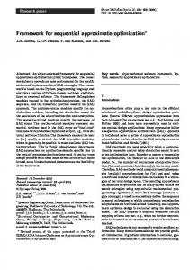
Model-based optimization methods construct a regression model (often called a response surface model) that predicts performance and then use this model for optimization. Sequential model-based optimization (SMBO) iterates between fitting a model and gathering additional data based on this model. In the context of parameter optimization, the model is fitted to a training set {(θ1 , o1 ), . . . , (θn , on )} where parameter configuration θi = (θi,1 , . . . , θi,d ) is a complete instantiation of the target algorithm’s d parameters and oi is the target algorithm’s observed performance when run with configuration θi . Given a new configuration θn+1 , the model aims to predict its performance on+1 . Sequential model-based optimization (SMBO) iterates between building a model and gathering additional data. We illustrate a simple SMBO procedure in Figure 1. Consider a deterministic algorithm A with a single continuous parameter x and let A’s runtime as a function of its parameter be described by the solid line in Figure 1(a). SMBO searches for a value of x that minimizes this runtime. Here, it is initialized by running A with the parameter values indicated by the circles in Figure 1(a). Next, SMBO fits a response surface model to the data gathered; Gaussian process (GP) models [20] are the most common choice. The black dotted line in Figure 1 represents the predictive mean of a GP model trained on the data given by the circles, and the shaded area around it quantifies the uncertainty in the predictions; this uncertainty grows with distance from the training data. SMBO uses this predictive performance model to select a promising parameter configuration for the next run of A. Promising configurations are predicted to perform well and/or lie in regions for which the model is still uncertain. These two objectives are

30

30 DACE mean prediction DACE mean +/− 2*stddev True function Function evaluations EI (scaled)

25

20

response y

response y

20

15

10

15

10

5

5

0

0

−5

DACE mean prediction DACE mean +/− 2*stddev True function Function evaluations EI (scaled)

25

0

0.2

0.4

0.6

parameter x

(a) SMBO, step 1

0.8

1

−5

0

0.2

0.4

0.6

0.8

1

parameter x

(b) SMBO, step 2

Fig. 1. Two steps of SMBO for the optimization of a 1D function. The true function is shown as a solid line, and the circles denote our observations. The dotted line denotes the mean prediction of a noise-free Gaussian process model (the “DACE” model), with the grey area denoting its uncertainty. Expected improvement (scaled for visualization) is shown as a dashed line.

combined in a so-called expected improvement (EI) criterion, which is high in regions of low predictive mean and high predictive variance (see the light dashed line in Figure 1(a); an exact formula for EI is given in Equation 3 in Section 4.3). SMBO selects a configuration with maximal EI (here, x = 0.705), runs A using it, and updates its model based on the result. In Figure 1(b), we show how this new data point changes the model: note the additional data point at x = 0.705, the greatly reduced uncertainty around it, and that the region of large EI is now split into two. While our example captures the essence of SMBO, recent practical SMBO instantiations include more complex mechanisms for dealing with randomness in the algorithm’s performance and for reducing the computational overhead. Algorithm Framework 1 gives the general structure of the time-bounded SMBO framework we employ in this paper. It starts by running the target algorithm with some initial parameter configurations, and then iterates three steps: (1) fitting a response surface model using the existing data; (2) selecting a list of promising configurations; and (3) running the target algorithm on (some of) the selected configurations until a given time bound is reached. This time bound is related to the combined overhead, tmodel + tei , due to fitting the model and selecting promising configurations. SMBO has is roots in the statistics literature on experimental design for global continuous (“black-box”) function optimization. Most notable is the efficient global optimization (EGO) algorithm by Jones et al.[15]; this is essentially the algorithm used in our simple example above. EGO is limited to optimizing continuous parameters for noise-free functions (i.e., the performance of deterministic algorithms). Follow-up work in the statistics community included an approach to optimize functions across multiple environmental conditions [21] as well as the sequential kriging optimization (SKO) algorithm for handling noisy functions (i.e., in our context, randomized algorithms) by Huang et al. [22]. In parallel to the latter work, Bartz-Beielstein et al. [16, 17] were the first to use the EGO approach to optimize algorithm performance. Their sequential

Algorithm Framework 1: Sequential Model-Based Optimization (SMBO) R keeps track of all target algorithm runs performed so far and their performances (i.e., ~ new SMBO’s training data {([θ1 , x1 ], o1 ), . . . , ([θn , xn ], on )}), M is SMBO’s model, Θ is a list of promising configurations, and tf it and tselect are the runtimes required to fit the model and select configurations, respectively. Input : Target algorithm A with parameter configuration space Θ; instance set Π; cost metric cˆ Output : Optimized (incumbent) parameter configuration, θinc 1 [R, θinc ] ← Initialize(Θ, Π); 2 repeat 3 [M, tf it ] ← FitModel(R); ~ new , tselect ] ← SelectConfigurations(M, θinc , Θ); 4 [Θ ~ new , θinc , M, R, tf it + tselect , Π, cˆ); 5 [R, θinc ] ← Intensify(Θ 6 until total time budget for configuration exhausted; 7 return θinc ;

parameter optimization (SPO) toolbox—which has received considerable attention in the evolutionary algorithms community—provides many features that facilitate the manual analysis and optimization of algorithm parameters; it also includes an automated SMBO procedure for optimizing continuous parameters on single instances. We started our own work in SMBO by comparing SKO vs SPO, studying their choices for the four SMBO components [18]. We demonstrated that component Intensify mattered most, and improved it in our SPO+ algorithm [18]. Subsequently, we showed how to reduce the overhead incurred by construction and use of response surface models via approximate GP models. We also eliminated the need for a costly initial design by interleaving randomly selected parameters throughout the optimization process instead and exploit that different algorithm runs take different amounts of time. The resulting time-bounded SPO variant, TB-SPO, is the first SMBO method practical for parameter optimization given a user-specified time budget [19]. Although it was shown to significantly outperform PARAM ILS on some domains, it is still limited to the optimization of continuous algorithm parameters on single problem instances. In the following, we generalize the components of the time-bounded SMBO framework (of which TB-SPO is an instantiation), extending its scope to tackle general algorithm configuration problems with many categorical parameters and sets of benchmark instances.

3

Randomized Online Aggressive Racing (ROAR)

In this section, we first generalize SMBO’s Intensify procedure to handle multiple instances, and then introduce ROAR, a very simple model-free algorithm configuration procedure based on this new intensification mechanism.

~ new , θinc , M, R, tintensif y , Π, cˆ) Procedure 2: Intensify(Θ cˆ(θ, Π 0 ) denotes the empirical cost of θ on the subset of instances Π 0 ⊆ Π, based on the runs in R; maxR is a parameter, set to 2 000 in all our experiments ~ new ; incumbent parameter setting, Input : Sequence of parameter settings to evaluate, Θ θinc ; model, M; sequence of target algorithm runs, R; time bound, tintensif y ; instance set, Π; cost metric, cˆ Output : Updated sequence of target algorithm runs, R; incumbent parameter setting, θinc ~ new ) do 1 for i := 1, . . . , length(Θ ~ new [i]; 2 θnew ← Θ 3 if R contains less than maxR runs with configuration θinc then 4 Π 0 ← {π 0 ∈ Π | R contains less than or equal number of runs using θinc and π 0 than using θinc and any other π 00 ∈ Π} ; 5 π ← instance sampled uniformly at random from Π 0 ; 6 s ← seed, drawn uniformly at random; 7 R ← ExecuteRun(R, θinc , π, s); 8 9 10 11 12 13 14 15 16 17 18 19

3.1

N ← 1; while true do Smissing ← hinstance, seedi pairs for which θinc was run before, but not θnew ; Storun ←random subset of Smissing of size min(N, |Smissing |); foreach (π, s) ∈ Storun do R ← ExecuteRun(R, θnew , π, s); Smissing ← Smissing \ Storun ; Πcommon ← instances for which we previously ran both θinc and θnew ; if cˆ(θnew , Πcommon ) > cˆ(θinc , Πcommon ) then break; else if Smissing = ∅ then θinc ← θnew ; break; else N ← 2 · N ; if time spent in this call to this procedure exceeds tintensif y and i ≥ 2 then break; return [R, θinc ];

Generalization I: An Intensification Mechanism for Multiple Instances

A crucial component of any algorithm configuration procedure is the so-called intensification mechanism, which governs how many evaluations to perform with each configuration, and when to trust a configuration enough to make it the new current best known configuration (the incumbent). When configuring algorithms for sets of instances, we also need to decide which instance to use in each run. To address this problem, we generalize TB-SPO’s intensification mechanism. Our new procedure implements a variance reduction mechanism, reflecting the insight that when we compare the empirical cost statistics of two parameter configurations across multiple instances, the variance in this comparison is lower if we use the same N instances to compute both estimates. Procedure 2 defines this new intensification mechanism more precisely. It takes as ~ new , and compares them in turn to the current input a list of promising configurations, Θ incumbent configuration until a time budget for this comparison stage is reached.1 1

~ new , one more configuration If that budget is already reached after the first configuration in Θ is used; see the last paragraph of Section 4.3 for an explanation why.

In each comparison of a new configuration, θnew , to the incumbent, θinc , we first perform an additional run for the incumbent, using a randomly selected hinstance, seedi combination. Then, we iteratively perform runs with θnew (using a doubling scheme) until either θnew ’s empirical performance is worse than that of θinc (in which case we reject θnew ) or we performed as many runs for θnew as for θinc and it is still at least as good as θinc (in which case we change the incumbent to θnew ). The hinstance, seedi combinations for θnew are sampled uniformly at random from those on which the incumbent has already run. However, every comparison in Procedure 2 is based on a different randomly selected subset of instances and seeds, while F OCUSED ILS’s Procedure “better” uses a fixed ordering to which it can be very sensitive.

3.2

Defining ROAR

We now define Random Online Aggressive Racing (ROAR), a simple model-free instantiation of the general SMBO framework (see Algorithm Framework 1).2 This surprisingly effective method selects parameter configurations uniformly at random and iteratively compares them against the current incumbent using our new intensification mechanism. We consider ROAR to be a racing algorithm, because it runs each candidate configuration only as long as necessary to establish whether it is competitive. It gets its name because the set of candidates is selected at random, each candidate is accepted or rejected online, and we make this online decision aggressively, before enough data has been gathered to support a statistically significant conclusion. More formally, as an instantiation of the SMBO framework, ROAR is completely specified by the four components Initialize, FitModel, SelectConfigurations, and Intensify. Initialize performs a single run with the target algorithm’s default parameter configuration (or a random configuration if no default is available) on an instance selected uniformly at random. Since ROAR is model-free, its FitModel procedure simply returns a constant model which is never used. SelectConfigurations returns a single configuration sampled uniformly at random from the parameter space, and Intensify is as described in Procedure 2.

4

Sequential Model-based Algorithm Configuration (SMAC)

In this section, we introduce our second, more sophisticated instantiation of the general SMBO framework: Sequential Model-based Algorithm Configuration (SMAC). SMAC can be understood as an extension of ROAR that selects configurations based on a model rather than uniformly at random. It instantiates Initialize and Intensify in the same way as ROAR. Here, we discuss the new model class we use in SMAC to support categorical parameters and multiple instances (Sections 4.1 and 4.2, respectively); then, we describe how SMAC uses its models to select promising parameter configurations (Section 4.3). Finally, we prove a convergence result for ROAR and SMAC (Section 4.4). 2

We previously considered random sampling approaches based on less powerful intensification mechanisms; see, e.g., R ANDOM∗ defined in [19].

4.1

Generalization II: Models for Categorical Parameters

The models in all existing SMBO methods of which we are aware are limited to numerical parameters. In this section, in order to handle categorical parameters, we adapt the most prominent previously used model class (Gaussian stochastic process models) and introduce the model class of random forests to SMBO. A Weighted Hamming Distance Kernel Function for GP Models. Most recent work on sequential model-based optimization [15, 16, 18] uses Gaussian stochastic process models (GPs; see [20]). GP models rely on a parameterized kernel function k : Θ ×Θ 7→ R+ that specifies the similarity between two parameter configurations. Previous SMBO approaches for numerical parameters typically choose the GP kernel function " d # X 2 k(θi , θj ) = exp (−λl · (θi,l − θj,l ) ) , (1) l=1

where λ1 , . . . , λd are the kernel parameters. For categorical parameters, we define a new, similar kernel. Instead of measuring the (weighted) squared distance, it computes a (weighted) Hamming distance: # " d X kcat (θi , θj ) = exp (−λl · [1 − δ(θi,l , θj,l )]) , (2) l=1

where δ is the Kronecker delta function (ones if its two arguments are identical and zero otherwise). For a combination of continuous parameters Pcont and categorical parameters Pcat , we apply the combined kernel " # X X 2 Kmixed (θi , θj ) = exp (−λl · (θi,l − θj,l ) ) + (−λl · [1 − δ(θi,l , θj,l )]) . l∈Pcont

l∈Pcat

Although Kmixed is a straightforward generalization of the standard Gaussian kernel in Equation 1, we are not aware of any prior use of this kernel or proof that it is indeed a valid kernel function.3 We provide this proof in the appendix. Since Gaussian stochastic processes are kernel-based learning methods and since Kmixed is a valid kernel function, it can be swapped in for the Gaussian kernel without changing any other component of the GP model. Here, we use the same projected process (PP) approximation of GP models [20] as in TB-SPO [19]. Random Forests. The new default model we use in SMAC is based on random forests [24], a standard machine learning tool for regression and classification. Random forests are collections of regression trees, which are similar to decision trees but have real 3

Couto [23] gives a recursive kernel function for categorical data that is related since it is also based on a Hamming distance.

values (here: target algorithm performance values) rather than class labels at their leaves. Regression trees are known to perform well for categorical input data; indeed, they have already been used for modeling the performance (both in terms of runtime and solution quality) of heuristic algorithms (e.g., [25, 26]). Random forests share this benefit and typically yield more accurate predictions [24]; they also allow us to quantify our uncertainty in a given prediction. We construct a random forest as a set of B regression trees, each of which is built on n data points randomly sampled with repetitions from the entire training data set {(θ1 , o1 ), . . . , (θn , on )}. At each split point of each tree, a random subset of dd · pe of the d algorithm parameters is considered eligible to be split upon; the split ratio p is a parameter, which we left at its default of p = 5/6. A further parameter is nmin , the minimal number of data points required to be in a node if it is to be split further; we use the standard value nmin = 10. Finally, we set the number of trees to B = 10 to keep the computational overhead small.4 We compute the random forest’s predictive mean µθ and variance σθ2 for a new configuration θ as the empirical mean and variance of its individual trees’ predictions for θ. Usually, the tree prediction for a parameter configuration θn+1 is the mean of the data points in the leaf one ends up in when propagating θn+1 down the tree. We adapted this mechanism to instead predict the user-defined cost metric of that data, e.g., the median of the data points in that leaf. Transformations of the Cost Metric. Model fit can often be improved by transforming the cost metric. In this paper, we focus on minimizing algorithm runtime. Previous work on predicting algorithm runtime has found that logarithmic transformations substantially improve model quality [27] and we thus use log-transformed runtime data throughout this paper; that is, for runtime ri , we use oi = ln(ri ). (SMAC can also be applied to optimize other cost metrics, such as the solution quality an algorithm obtains in a fixed runtime; other transformations may prove more efficient for other metrics.) However, we note that in some models such transformations implicitly change the cost metric users aim to optimize. For example, take a simple case where there is only one parameter configuration θ for which we measured runtimes (r1 , . . . , r10 )=(21 , 22 , . . . , 210 ). While the true arithmetic mean of these runs is roughly 205, a GP model trained on this data using a log transformation would predict the mean to be exp (mean((log(r1 ), . . . , log(r10 )))) ≈ 45. This is because the arithmetic mean of the logs is the log of the geometric mean: v " !#(1/n) u n n X uY n geometric mean = t xi = exp log(xi ) i=1

" = exp

i=1 n

#

1X log(xi ) = exp (mean of logs). n i=1

For GPs, it is not clear how to fix this problem. We avoid this problem in our random forests by computing the prediction in the leaf of a tree by “untransforming” the data, computing the user-defined cost metric, and then transforming the result again. 4

An optimization of these three parameters might improve performance further. We plan on studying this in the context of an application of SMAC to optimizing its own parameters.

4.2

Generalization III: Models for Sets of Problem Instances

There are several possible ways to extend SMBO’s models to handle multiple instances. Most simply, one could use a fixed set of N instances for every evaluation of the target algorithm run, reporting aggregate performance. However, there is no good fixed choice for N : small N leads to poor generalization to test data, while large N leads to a prohibitive N -fold slowdown in the cost of each evaluation. (This is the same problem faced by the PARAM ILS instantiation BASIC ILS(N) [8].) Instead, we explicitly integrate information about the instances into our response surface models. Given a vector of features xi describing each training problem instance πi ∈ Π, we learn a joint model that predicts algorithm runtime for combinations of parameter configurations and instance features. We then aggregate these predictions across instances. Instance Features. Existing work on empirical hardness models [28] has demonstrated that it is possible to predict algorithm runtime based on features of a given problem instance. Most notably, such predictions have been exploited to construct portfolio-based algorithm selection mechanisms, such as SATzilla [29, 27]. For SAT instances in the form of CNF formulae, we used 126 features including features based on graph representations of the instance, an LP relaxation, DPLL probing, local search probing, clause learning, and survey propagation. All features are listed in Figure 2. For MIP instances we computed 39 features, including features based on graph representations, an LP relaxation, the objective function, and the linear constraint matrix. All features are listed in Figure 3. To reduce the computational complexity of learning, we applied principal component analysis (see, e.g., [30]), to project the feature matrix into a lower-dimensional subspace spanned by the seven orthogonal vectors along which it has maximal variance. For new domains, for which no features have yet been defined, SMAC can still be applied with an empty feature set or simple domain-independent features, such as instance size or the performance of the algorithm’s default setting (which, based on preliminary experiments, seems to be a surprisingly effective feature). Note that in contrast to per-instance approaches, such as SATzilla [29, 27], instance features are only needed for the training instances: the end result of algorithm configuration is a single parameter configuration that is used without a need to compute features for test instances. As a corollary, the time required for feature computation is not as crucial in algorithm configuration as it is in per-instance approaches: in per-instance approaches, feature computation has to be counted as part of the time required to solve test instances, while in algorithm configuration no features are computed for test instances at all. In fact, features for the training instances may well be the result of an extensive offline analysis of those training instances, or can even be taken from the literature. Computing the features we used here took an average of 30 seconds for the SAT domains, and 4.4 seconds for the MIP domains. Predicting Performance Across Instances. So far, we have discussed models trained on pairs (θi , oi ) of parameter configurations θi and their observed performance oi . Now, we extend this data to include instance features. Let xi denote the vector of

61.–62. Search space size estimate: mean depth Problem Size Features: to contradiction, estimate of the log of 1.–2. Number of variables and clauses in orignumber of nodes inal formula: denoted v and c, respectively 3.–4. Number of variables and clauses after LP-Based Features: simplification with SATelite: denoted v’ 63.–66. Integer slack vector: mean, variation coand c’, respectively efficient, min, and max 5.–6. Reduction of variables and clauses by 67. Ratio of integer variables in LP solution simplification: (v-v’)/v’ and (c-c’)/c’ 68. Objective function value of LP solution 7. Ratio of variables to clauses: v’/c’ Local Search Probing Features, based on 2 Variable-Clause Graph Features: seconds of running each of SAPS and GSAT: 8.–12. Variable node degree statistics: mean, variation coefficient, min, max, and entropy 69.–78. Number of steps to the best local min13.–17. Clause node degree statistics: mean, imum in a run: mean, median, variation variation coefficient, min, max, and encoefficient, 10th and 90th percentiles tropy 79.–82. Average improvement to best in a run: mean and coefficient of variation of imVariable Graph Features: provement per step to best solution 18–21. Node degree statistics: mean, variation 83.–86. Fraction of improvement due to first locoefficient, min, and max cal minimum: mean and variation coeffi22.–26. Diameter: mean, variation coefficient, cient min, max, and entropy 87.–90. Coefficient of variation of the number 27.–31. Clustering Coefficient: mean, variation of unsatisfied clauses in each local minicoefficient, min, max, and entropy mum: mean and variation coefficient Clause Graph Features: Clause Learning Features (based on 2 sec32–36. Node degree statistics: mean, variation onds of running Zchaff rand): coefficient, min, max, and entropy 91.–99. Number of learned clauses: mean, variBalance Features: ation coefficient, min, max, 10%, 25%, 37.–41. Ratio of positive to negative literals in 50%, 75%, and 90% quantiles each clause: mean, variation coefficient,100.–108. Length of learned clauses: mean, variation coefficient, min, max, 10%, 25%, min, max, and entropy 42.–46. Ratio of positive to negative occur50%, 75%, and 90% quantiles rences of each variable: mean, variation coefficient, min, max, and entropy Survey Propagation Features 47.–49. Fraction of unary, binary, and ternary 109.–117. Confidence of survey propagation: For clauses each variable, compute the higher of P (true)/P (f alse) or P (f alse)/P (true). Proximity to Horn Formula: Then compute statistics across variables: 50. Fraction of Horn clauses 51.–55. Number of occurrences in a Horn clause mean, variation coefficient, min, max, for each variable: mean, variation coeffi10%, 25%, 50%, 75%, and 90% quantiles 118.–126. Unconstrained variables: For each varicient, min, max, and entropy able, compute P (unconstrained). Then DPLL Probing Features: compute statistics across variables: mean, 56.–60. Number of unit propagations: computed variation coefficient, min, max, 10%, at depths 1, 4, 16, 64 and 256 25%, 50%, 75%, and 90% quantiles

Fig. 2. 11 groups of SAT features; these were introduced in [29, 27, 31].

features for the instance used in the ith target algorithm run. Concatenating parameter values, θi , and instance features, xi , into one input vector yields the training data {([θ1 , x1 ], o1 ), . . . , ([θn , xn ], on )}. From this data, we learn a model that takes as input a parameter configuration θ and predicts performance across all training instances. For GP models, there exists an approach from the statistics literature to predict mean

Problem Size Features: 1.–2. Number of variables and constraints: denoted n and m, respectively 3. Number of nonzero entries in the linear constraint matrix, A

26. Standard deviation of {ci /ni }n i=1 , where ni denotes the number of nonzero entries in column i of A √ 27. Standard deviation of {ci / ni }n i=1 Linear Constraint Matrix Features:

Variable-Constraint Graph Features:

28.–29. Distribution of normalized constraint matrix entries, Ai,j /bi : mean and stddev 4–7. Variable node degree statistics: mean, (only of elements where bi 6= 0) max, min, and stddev 30.–31. Variation coefficient of normalized abso8–11. Constraint node degree statistics: mean, lute nonzero entries per row: mean and max, min, and stddev stddev Variable Graph (VG) Features:

Variable Type Features: 12–17. Node degree statistics: max, min, stddev, 32.–33. Support size of discrete variables: mean 25% and 75% quantiles and stddev 18–19. Clustering Coefficient: mean and stddev 34. Percent unbounded discrete variables 20. Edge Density: number of edges in the VG 35. Percent continuous variables divided by the number of edges in a complete graph having the same number of General Problem Type Features: nodes LP-Based Features: 21–23. Integer slack vector: mean, max, L2 norm 24. Objective function value of LP solution Objective Function Features: 25. Standard deviation of normalized coefficients: {ci /m}n i=1

36. Problem type: categorical feature attributed by CPLEX (LP, MILP, FIXEDMILP, QP, MIQP, FIXEDMIQP, MIQP, QCP, or MIQCP) 37. Number of quadratic constraints 38. Number of nonzero entries in matrix of quadratic coefficients of objective function, Q 39. Number of variables with nonzero entries in Q

Fig. 3. Eight groups of features for the mixed integer programming problem. These general MIP features have been introduced in [11] as a generalization of features for the combinatorial winner determination problem in [32].

performance across problem instances [21]. However, due to the issue discussed in Section 4.1, when using log transformations this approach would not model the cost metric the user specifies; e.g., instead of the arithmetic mean it would model geometric mean. This problem would be particularly serious in the case of multiple instances, as performance often varies by orders of magnitude from one instance to another. As a consequence, we did not implement a version of SMAC(PP) for multiple instances at this time. Instead, we adapted RF models to handle predictions across multiple instances. All input dimensions are handled equally when constructing the random forest, regardless of whether they refer to parameter values or instance features. The prediction procedure changes as follows: within each tree, we first predict performance for the combinations of the given parameter configuration and each instance; next, we combine these predictions with the user-defined cost metric (e.g., arithmetic mean runtime); finally, we compute means and variances across trees.

4.3

Generalization IV: Using the Model to Select Promising Configurations in Large Mixed Numerical/Categorical Configuration Spaces

The SelectConfiguration component in SMAC uses the model to select a list of promising parameter configurations. To quantify how promising a configuration θ is, it uses the model’s predictive distribution for θ to compute its expected positive improvement (EI(θ)) [15] over the best configuration seen so far (the incumbent). EI(θ) is large for configurations θ with low predicted cost and for those with high predicted uncertainty; thereby, it offers an automatic tradeoff between exploitation (focusing on known good parts of the space) and exploration (gathering more information in unknown parts of the space). Specifically, we use the E[Iexp ] criterion introduced in [18] for log-transformed costs; given the predictive mean µθ and variance σθ2 of the log-transformed cost of a configuration θ, this is defined as 1

2

EI(θ) := E[Iexp (θ)] = fmin Φ(v) − e 2 σθ +µθ · Φ(v − σθ ),

(3)

)−µθ where v := ln(fmin , Φ denotes the cumulative distribution function of a standard σθ normal distribution, and fmin denotes the empirical mean performance of θinc .5 Having defined EI(θ), we must still decide how to identify configurations θ with large EI(θ). This amounts to a maximization problem across parameter configuration space. Previous SMBO methods [16, 17, 18, 19] simply applied random sampling for this task (in particular, they evaluated EI for 10 000 random samples), which is unlikely to be sufficient in high-dimensional configuration spaces, especially if promising configurations are sparse. To gather a set of promising configurations with low computational overhead, we perform a simple multi-start local search and consider all resulting configurations with locally maximal EI.6 This search is similar in spirit to PARAM ILS [8, 9], but instead of algorithm performance it optimizes EI(θ) (see Equation 3), which can be evaluated based on the model predictions µθ and σθ2 without running the target algorithm. More concretely, the details of our local search are as follows. We compute EI for all configuations used in previous target algorithm runs, pick the ten configurations with maximal EI, and initialize a local search at each of them. To seamlessly handle mixed categorical/numerical parameter spaces, we use a randomized one-exchange neighbourhood, including the set of all configurations that differ in the value of exactly one discrete parameter, as well as four random neighbours for each numerical parameter. In particular, we normalize the range of each numerical parameter to [0,1] and then sample four “neighbouring” values for numerical parameters with current value v from a univariate Gaussian distribution with mean v and standard deviation 0.2, rejecting new values outside the interval [0,1]. Since batch model predictions (and thus batch EI computations) for a set of N configurations are much cheaper than separate predictions for N configurations, we use a best improvement search, evaluating EI for all neighbours at once; we stop each local search once none of the neighbours has larger EI. Since 5

6

In TB-SPO [19], we used fmin = µ(θinc ) + σ(θinc ). However, we now believe that setting fmin to the empirical mean performance of θinc yields better performance overall. We plan to investigate better mechanisms in the future. However, we note that the best problem formulation is not obvious, since we desire a diverse set of configurations with high EI.

SMBO sometimes evaluates many configurations per iteration and because batch EI computations are cheap, we simply compute EI for an additional 10 000 randomly-sampled configurations; we then sort all 10 010 configurations in descending order of EI. (The ten results of local search typically had larger EI than all randomly sampled configurations.) Having selected this list of 10 010 configurations based on the model, we interleave randomly-sampled configurations in order to provide unbiased training data for future models. More precisely, we alternate between configurations from the list and additional configurations sampled uniformly at random. 4.4

Theoretical Analysis of SMAC and ROAR

In this section, we provide a convergence proof for SMAC (and ROAR) for finite configuration spaces. Since Intensify always compares at least two configurations against the current incumbent, at least one randomly sampled configuration is evaluated in every iteration of SMBO. In finite configuration spaces, thus, each configuration has a positive probability of being selected in each iteration. In combination with the fact that Intensify increases the number of runs used to evaluate each configuration unboundedly, this allows us to prove that SMAC (and ROAR) eventually converge to the optimal configuration when using consistent estimators of the user-defined cost metric. The proof is straight-forward, following the same arguments as a previous proof about FocusedILS (see [9]). Nevertheless, we give it here for completeness. Definition 1 (Consistent estimator) cˆN (θ) is a consistent estimator for c(θ) iff ∀ > 0 : lim P (|ˆ cN (θ) − c(θ)| < ) = 1. N →∞

When we estimate that a parameter configuration’s true cost c(θ) based on N runs is cˆN (θ), and when cˆN (θ) is a consistent estimator of c(θ), cost estimates become increasingly reliable as N approaches infinity, eventually eliminating the possibility of mistakes in comparing two parameter configurations. The following lemma is exactly Lemma 8 in [9]; for the proof, see that paper. Lemma 2 (No mistakes for N → ∞) Let θ1 , θ2 ∈ Θ be any two parameter configurations with c(θ1 ) < c(θ2 ). Then, for consistent estimators cˆN , limN →∞ P (ˆ cN (θ1 ) ≥ cˆN (θ2 )) = 0. All that remains to be shown is that SMAC evaluates each parameter configuration an unbounded number of times. Lemma 3 (Unbounded number of evaluations) Let N (J, θ) denote the number of runs SMAC has performed with parameter configuration θ at the end of SMBO iteration J. Then, if SMBO’s parameter maxR is set to ∞, for any constant K and configuration θ ∈ Θ (with finite Θ), limJ→∞ P [N (J, θ) ≥ K] = 1. Proof. In each SMBO iteration, SMAC evaluates at least one random configuration (performing at least one new run for it since maxR = ∞), and with a probability of p = 1/|Θ|, this is configuration θ. Hence, the number of runs performed with θ is lower-bounded by a binomial random variable B(k; J, p). Then, for any constant k < K we obtain limJ→∞ B(k; J, p) Thus, limJ→∞ P [N (J, θ) ≥ K] = 1.

Theorem 4 (Convergence of SMAC) When SMAC with maxR = ∞ optimizes a cost measure c based on a consistent estimator cˆN and a finite configuration space Θ, the probability that it finds the true optimal parameter configuration θ ∗ ∈ Θ approaches one as the time allowed for configuration goes to infinity. Proof. Each SMBO iteration takes finite time. Thus, as time goes to infinity so does the number of SMBO iterations, J. According to Lemma 3, as J goes to infinity N (θ) grows unboundedly for each θ ∈ Θ. For each θ1 , θ2 , as N (θ1 ) and N (θ2 ) go to infinity, Lemma 2 states that in a pairwise comparison, the truly better configuration will be preferred. Thus eventually, SMAC visits all finitely many parameter configurations and prefers the best one over all others with probability arbitrarily close to one. We note that this convergence result holds regardless of the model type used. In fact, it even holds for a simple round robin procedure that loops through parameter configurations. We thus rely on empirical results to assess SMAC. We present these in the following sections, after explaining how to build the relevant models.

5

Experimental Evaluation

We now compare the performance of SMAC, ROAR, TB-SPO [19], GGA [10], and PARAM ILS (in particular, F OCUSED ILS 2.3) [9] for a wide variety of configuration scenarios, aiming to target algorithm runtime for solving SAT and MIP problems. In principle, our ROAR and SMAC methods also apply to optimizing other cost metrics, such as the solution quality an algorithm can achieve in a fixed time budget; we plan on studying their empirical performance for this case in the near future. 5.1

Experimental Setup

Configuration scenarios. We used 17 configuration scenarios from the literature, involving the configuration of the local search SAT solver SAPS [33] (4 parameters), the tree search solver SPEAR [34] (26 parameters), and the most widely used commercial mixed integer programming solver, IBM ILOG CPLEX7 (76 parameters). SAPS is a dynamic local search algorithm, and its four continuous parameters control the scaling and smoothing of clause weights, as well as the percentage of random steps. We use its UBCSAT implementation [35]. SPEAR is a tree search algorithm for SAT solving developed for industrial instances, and with appropriate parameter settings it is the best available solver for certain types of SAT-encoded hardware and software verification instances [13]. SPEAR has 26 parameters, including ten categorical, four integer, and twelve continuous parameters. The categorical parameters mainly control heuristics for variable and value selection, clause sorting, resolution ordering, and also enable or disable optimizations, such as the pure literal rule. The continuous and integer parameters mainly deal with activity, decay, and elimination of variables and clauses, as well as with the interval of randomized restarts and percentage of random choices. CPLEX is the most-widely used commercial optimization tool for solving MIPs, currently used 7

http://ibm.com/software/integration/optimization/cplex-optimizer

by over 1 300 corporations and government agencies, along with researchers at over 1 000 universities. In defining CPLEX’s configuration space, we were careful to keep all parameters fixed that change the problem formulation (e.g., parameters such as the optimality gap below which a solution is considered optimal). The 76 parameters we selected affect all aspects of CPLEX. They include 12 preprocessing parameters (mostly categorical); 17 MIP strategy parameters (mostly categorical); 11 categorical parameters deciding how aggressively to use which types of cuts; 9 numerical MIP “limits” parameters; 10 simplex parameters (half of them categorical); 6 barrier optimization parameters (mostly categorical); and 11 further parameters. Most parameters have an “automatic” option as one of their values. We allowed this value, but also included other values (all other values for categorical parameters, and a range of values for numerical parameters). In all 17 configuration scenarios, we terminated target algorithm runs at κmax = 5 seconds, the same per-run cutoff time used in previous work for these scenarios. In previous work, we have also applied PARAM ILS to optimize MIP solvers with very large per-run captimes (up to κmax = 10 000s), and obtained better results than the CPLEX tuning tool [1]. We believe that for such large captimes, an adaptive capping mechanism, such as the one implemented in ParamILS [9], is essential; we are currently working on integrating such a mechanism into SMAC.8 In this paper, to study the remaining components of SMAC, we only use scenarios with small captimes of 5s. In order to enable a fair comparison with GGA, we changed the optimization objective of all 17 scenarios from the original PAR-10 (penalized average runtime, counting timeouts at κmax as 10·κmax , which is not supported by GGA) to simple average runtime (PAR-1, counting timeouts at κmax as κmax ). 9 However, one difference remains: we minimize the runtime reported by the target algorithm, but GGA can only minimize its own measurement of target algorithm runtime, including (sometimes large) overheads for reading in the instance. All instances we used are available at http://www.cs.ubc.ca/ labs/beta/Projects/AAC.

Parameter transformations. Some numerical parameters naturally vary on a nonuniform scale (e.g., a parameter θ with an interval [100, 1600] that we discretized to the values {100, 200, 400, 800, 1600} for use in PARAM ILS). We transformed such parameters to a domain in which they vary more uniformly (e.g., log(θ) ∈ [log(100), log(1600)]), un-transforming the parameter values for each call to the target algorithm. 8

In fact, preliminary experiments for configuration scenario CORLAT (from [1], with κmax = 10 000s) highlight the importance of developing an adaptive capping mechanism for SMAC: e.g., in one of SMAC’s run, it only performed 49 target algorithm runs, with 15 of them timing out after κmax = 10 000s, and another 3 taking over 5 000 seconds each. Together, these runs exceeded the time budget of 2 CPU days (172 800 seconds), despite the fact that all of them could have safely been cut off after less than 100 seconds. As a result, for scenario CORLAT, SMAC performed a factor of 3 worse than PARAM ILS with κmax = 10 000s. On the other hand, SMAC can sometimes achieve strong performance even with relatively high captimes; e.g., on CORLAT with κmax = 300s, SMAC outperformed PARAM ILS by a factor of 1.28. 9 Using PAR-10 to compare the remaining configurators, our qualitative results did not change.

Comparing configuration procedures. We performed 25 runs of each configuration procedure on each configuration scenario. For each such run ri , we computed test performance ti as follows. First, we extracted the incumbent configuration θinc at the point the configuration procedure exhausted its time budget; SMAC’s overhead due to the construction and use of models were counted as part of this budget. Next, in an offline evaluation step using the same per-run cutoff time as during training, we measured the mean runtime ti across 1 000 independent test runs of the target algorithm parameterized by θinc . In the case of multiple-instance scenarios, we used a test set of previously unseen instances. For a given scenario, this resulted in test performances t1 , . . . , t25 for each configuration procedure. We report medians across these 25 values, visualize their variance in boxplots, and perform a Mann-Whitney U test to check for significant differences between configuration procedures. We ran GGA through HAL [36], using parameter settings recommended by GGA’s author, Kevin Tierney, in e-mail communication: we set the population size to 70, the number of generations to 100, the number of runs to perform in the first generation to 5, and the number of runs to perform in the last generation to 70. We used default settings for F OCUSED ILS 2.3, including aggressive capping. We note that in a previous comparison [10] of GGA and F OCUSED ILS, capping was disabled in F OCUSED ILS; this explains its poor performance there and its better performance here. With the exception of F OCUSED ILS, all of the configuration procedures we study here support numerical parameters without a need for discretization. We present results both for the mixed numerical/categorical parameter space these methods search, and—to enable a direct comparison to F OCUSED ILS—for a fully discretized configuration space. Computational environment. We conducted all experiments on a cluster of 55 dual 3.2GHz Intel Xeon PCs with 2MB cache and 2GB RAM, running OpenSuSE Linux 11.1. We measured runtimes as CPU time on these reference machines. 5.2

Experimental Results for Single Instance Scenarios

In order to evaluate our new general algorithm configuration procedures ROAR and SMAC one component at a time, we first evaluated their performance for optimizing the continuous parameters of SAPS and the mixed numerical/categorical parameters of SPEAR on single SAT instances; multi-instance scenarios are studied in the next section. To enable a comparison with our previous SMBO instantiation TB-SPO, we used the 6 configuration scenarios introduced in [19], which aim to minimize SAPS’s runtime on 6 single SAT-encoded instances, 3 each from quasigroup completion (QCP [37]) and from small world graph colouring (SWGCP [38]). We also used 5 similar new configuration scenarios, which aim to optimize SPEAR for 5 further SAT-encoded instances: 3 from software verification (SWV [39]) and 2 from IBM bounded model checking (IBM [40]; we only used 2 low quantiles of this hard distribution since SPEAR could not solve the instance at the 75% quantile within the cutoff time). The configuration scenarios are named algorithm-distribution-quantile: e.g., S A P S -QCP- M E D aims to optimize SAPS performance on a median-hard QCP instance. The time budget for each algorithm configuration run was 30 CPU minutes, exactly following [19].

The model-based approaches SMAC and TB-SPO performed best in this comparison, followed by ROAR, F OCUSED ILS, and GGA. Table 1 shows the results achieved by each of the configuration procedures, for both the full parameter configuration space (which includes numerical parameters) and the discretized version we made for use with F OCUSED ILS. For the special case of single instances and a small number of allnumerical parameters, SMAC(PP) and TB-SPO are very similar, and both performed best.10 While TB-SPO does not apply in the remaining configuration scenarios, our more general SMAC method achieved the best performance in all of them. For all-numerical parameters, SMAC performed slightly better using PP models, while in the presence of categorical parameters the RF models performed better. ROAR performed well for small but not for large configuration spaces: it was among the best (i.e., best or not significantly different from the best) in most of the SAPS scenarios (4 parameters) but only for one of the SPEAR scenarios (26 parameters). Both GGA and F OCUSED ILS performed slightly worse than ROAR for the SAPS scenarios, and slightly (but statistically significantly) worse than SMAC for most SPEAR configuration scenarios. Figure 4 visualizes each configurator’s 25 test performances for all scenarios. We note that SMAC and ROAR often yielded more robust results than F OCUSED ILS and GGA: for many scenarios some of the 25 F OCUSED ILS and GGA runs did very poorly. Our new SMAC and ROAR methods were able to explore the full configuration space, which sometimes led to substantially improved performance compared to the discretized configuration space PARAM ILS is limited to. Comparing the left vs the right side of Table 1, we note that the SAPS discretization (the same we used to optimize SAPS with PARAM ILS in previous work [8, 9]) left substantial room for improvement when exploring the full space: roughly 1.15-fold and 1.55-fold speedups on the QCP and SWGCP instances, respectively. GGA did not benefit as much from being allowed to explore the full configuration space for the SAPS scenarios; however, in one of the SPEAR scenarios (S P E A R -IBM- M E D ), it did perform 1.15 times better for the full space (albeit still worse than SMAC). 5.3

Experimental Results for General Multi-Instance Configuration Scenarios

We now compare the performance of SMAC, ROAR, GGA, and F OCUSED ILS on six general algorithm configuration tasks that aim to minimize the mean runtime of SAPS, SPEAR, and CPLEX for various sets of instances. These are the 5 B R O A D configuration scenarios used in [9] to evaluate PARAM ILS’s performance, plus one further CPLEX scenario, and we used the same time budget of 5 hours per configuration run. These instances come from the following domains: quasigroup completion, QCP [37]; small world graph colouring, SWGCP [38]; winner determination in combinatorial auctions, R EGIONS 100 [41]; mixed integer knapsack, MIK [42]. Overall, SMAC performed best in this comparison: as shown in Table 2 its performance was among the best (i.e., statistically indistinguishable from the best) in all 6 configuration scenarios, for both the discretized and the full configuration spaces. Our simple ROAR method performed surprisingly well, indicating the importance of the 10

In this special case, the two only differ in the expected improvement criterion and its optimization.

Scenario

Unit

S A P S -QCP- M E D S A P S -QCP- Q 075 S A P S -QCP- Q 095 S A P S -SWGCP- M E D S A P S -SWGCP- Q 075 S A P S -SWGCP- Q 095 S P E A R -IBM- Q 025 S P E A R -IBM- M E D S P E A R -SWV- M E D S P E A R -SWV- Q 075 S P E A R -SWV- Q 095

[·10−2 s] [·10−1 s] [·10−1 s] [·10−1 s] [·10−1 s] [·10−1 s] [·10−1 s] [·100 s] [·10−1 s] [·10−1 s] [·10−1 s]

Full configuration space SMAC SMAC(PP) TB-SPO ROAR 4.70 4.54 4.58 4.72 2.29 2.21 2.22 2.34 1.37 1.35 1.35 1.55 1.61 1.65 1.63 1.7 2.11 2.2 2.48 2.32 2.36 2.56 2.69 2.49 6.24 6.31 — 6.31 3.28 3.07 — 3.36 6.04 6.12 — 6.11 5.76 5.83 — 5.88 8.38 8.5 — 8.55

GGA 6.28 2.74 1.75 2.48 3.19 3.13 6.33 3.35 6.14 5.83 8.47

Discretized configuration space SMAC SMAC(PP) ROAR F-ILS GGA 5.27 5.27 5.25 5.50 6.24 2.87 2.93 2.92 2.91 2.98 1.51 1.58 1.57 1.57 1.95 2.54 2.59 2.58 2.57 2.71 3.26 3.41 3.38 3.55 3.55 3.65 3.78 3.79 3.75 3.77 6.21 6.27 6.30 6.31 6.30 3.16 3.18 3.38 3.47 3.84 6.05 6.12 6.14 6.11 6.15 5.76 5.89 5.89 5.88 5.84 8.42 8.51 8.53 8.58 8.49

Table 1. Comparison of algorithm configuration procedures for optimizing parameters on single problem instances. We performed 25 independent runs of each configuration procedure and report the median of the 25 test performances (mean runtimes across 1 000 target algorithm runs with the found configurations). We bold-faced entries for configurators that are not significantly worse than the best configurator for the respective configuration space, based on a Mann-Whitney U test. The symbol “—” denotes that the configurator does not apply for this configuration space.

2.5

0.15

0.25 0.2

0.6

0.25

1.5

0.4

0.4

0.2

0.05

QCPmed

0.6

0.3

0.3

S P T R F G

0.8

0.35

2 0.1

0.8

0.4

0.35

QCP−q075

0.2

0.15

1 S P T R F G

S

P

T

R

F G

QCP−q095

S P T R F G

0.2 S

SWGCP−med

P

T

R

F G

S

SWGCP−q075

P

T

R

F G

SWGCP−q095

(a) SAPS (4 continuous parameters) 0.68

4.5

0.66

2.5

0.63

4

0.62

3.5

0.64

0.61

3

0.62 P R F IBMq025

G

S

P R F IBMmed

G

3

1.5

2

1 1

0.5

0.6

2.5 S

2

S

P R F SWVmed

G

S

P R F SWVq075

G

S

P R F SWVq095

G

(b) SPEAR (26 parameters; 12 of them continuous and 4 integral) Fig. 4. Visual comparison of configuration procedures’ performance for setting SAPS and SPEAR’s parameters for single instances. For each configurator and scenario, we show boxplots for the 25 test performances underlying Table 1, for the full configuration space (discretized for F OCUSED ILS). ‘S’ stands for SMAC, ‘P’ for SMAC(PP), ‘T’ for TB-SPO, ‘R’ for ROAR, ‘F’ for F OCUSED ILS, and ‘G’ for GGA.

intensification mechanism: it was among the best in 2 of the 6 configuration scenarios for either version of the configuration space. However, it performed substantially worse than the best approaches for configuring CPLEX—the algorithm with the largest configuration space; we note that ROAR’s random sampling approach lacks the guidance offered by either F OCUSED ILS’s local search or SMAC’s response surface model. GGA performed

Scenario

Unit

S A P S -QCP S A P S -SWGCP S P E A R -QCP S P E A R -SWGCP CPLEX-R E G I O N S 100 CPLEX-MIK

[·10−1 s] [·10−1 s] [·10−1 s] [·100 s] [·10−1 s] [·100 s]

Full configuration space SMAC ROAR F-ILS GGA 7.05 7.52 — 7.84 1.77 1.8 — 2.82 1.65 1.84 — 2.21 1.16 1.16 — 1.17 3.45 6.67 — 4.37 1.20 2.81 — 3.42

Discretized configuration space SMAC ROAR F-ILS GGA 7.65 7.65 7.62 7.59 2.94 3.01 2.91 3.04 1.93 2.01 2.08 2.01 1.16 1.16 1.18 1.18 3.50 7.23 3.23 3.98 1.24 3.11 2.71 3.32

Table 2. Comparison of algorithm configuration procedures for benchmarks with multiple instances. We performed 25 independent runs of each configuration procedure and report the median of the 25 test performances (mean runtimes across 1 000 target algorithm runs with the found configurations on a test set disjoint from the training set). We bold-face entries for configurators that are not significantly worse than the best configurator for the respective configuration space, based on a Mann-Whitney U test.

slightly better for optimizing CPLEX than ROAR, but also significantly worse than either F OCUSED ILS or SMAC. Figure 5 visualizes the performance each configurator achieved for all 6 scenarios. We note that—similarly to the single instance cases—the results of SMAC were often more robust than those of F OCUSED ILS and GGA. Although the performance improvements achieved by our new methods might not appear large in absolute terms, it is important to remember that algorithm configuration is an optimization problem, and that the ability to tease out the last few percent of improvement often distinguishes good algorithms. We expect the difference between configuration procedures to be clearer in scenarios with larger per-instance runtimes. In order to handle such scenarios effectively, we believe that SMAC will require an adaptive capping mechanism similar to the one we introduced for PARAM ILS [9]; we are actively working on integrating such a mechanism with SMAC’s models. As in the single-instance case, for some configuration scenarios, SMAC and ROAR achieved much better results when allowed to explore the full space rather than F OCUSED ILS’s discretized search space. Speedups for SAPS were similar to those observed in the single-instance case (about 1.15-fold for S A P S -QCP and 1.65-fold for S A P S -SWGCP), but now we also observed a 1.17-fold improvement for S P E A R -QCP. In contrast, GGA actually performed worse for 4 of the 6 scenarios when allowed to explore the full space.

6

Conclusion

In this paper, we extended a previous line of work on sequential model-based optimization (SMBO) to tackle general algorithm configuration problems. SMBO had previously been applied only to the optimization of algorithms with numerical parameters on single problem instances. Our work overcomes both of these limitations, allowing categorical parameters and configuration for sets of problem instances. The four technical advances that made this possible are (1) a new intensification mechanism that employs blocked comparisons between configurations; an alternative class of response surface models, random forests, to handle (2) categorical parameters and (3) multiple instances; and (4) a new optimization procedure to select the most promising parameter configuration in a large mixed categorical/numerical space.

0.9 0.3

1.35

0.8

0.4 0.8

0.25 0.3

0.7

0.2 0.2

0.15

0.6

1.3

0.7

1.25

0.6

1.2

0.5

1.15

0.4

4 3 2 1

0.3 S

R

F

SAPS−QCP

G

S

R

F

G

SAPS−SWGCP

S

R

F

G

SPEAR−QCP

S

R

F

G

SPEAR−SWGCP

S

R

F

G

CPLEX−regions100

S

R

F

CPLEX−MIK

G

Fig. 5. Visual comparison of configuration procedures for general algorithm configuration scenarios. For each configurator and scenario, we show boxplots for the runtime data underlying Table 2, for the full configuration space (discretized for F OCUSED ILS). ‘S’ stands for SMAC, ‘R’ for ROAR, ‘F’ for F OCUSED ILS, and ‘G’ for GGA. F OCUSED ILS does not apply for the full configuration space, denoted by “—”.

We presented empirical results for the configuration of two SAT algorithms (one local search, one tree search) and the commercial MIP solver CPLEX on a total of 17 configuration scenarios, demonstrating the strength of our methods. Overall, our new SMBO procedure SMAC yielded statistically significant—albeit sometimes small— improvements over all of the other approaches on several configuration scenarios, and never performed worse. In contrast to F OCUSED ILS, our new methods are also able to search the full (non-discretized) configuration space, which led to further substantial improvements for several configuration scenarios. We note that our new intensification mechanism enabled even ROAR, a simple model-free approach, to perform better than previous general-purpose configuration procedures in many cases; ROAR only performed poorly for optimizing CPLEX, where good configurations are sparse. SMAC yielded further improvements over ROAR and—most importantly—also state-of-the-art performance for the configuration of CPLEX. In future work, we plan to improve SMAC to better handle configuration scenarios with large per-run captimes for each target algorithm run; specifically, we plan to integrate PARAM ILS’s adaptive capping mechanism into SMAC, which will require an extension of SMACs models to handle the resulting partly censored data. While in this paper we aimed to find a single configuration with overall good performance, we also plan to use SMAC’s models to determine good configurations on a per-instance basis. Finally, we plan to use these models to characterize the importance of individual parameters and their interactions, and to study interactions between parameters and instance features.

Acknowledgements We thank Kevin Murphy for many useful discussions on the modelling aspect of this work. Thanks also to Chris Fawcett and Chris Nell for help with running GGA through HAL, to Kevin Tierney for help with GGA’s parameters, and to James Styles and Mauro Vallati for comments on an earlier draft of this paper. FH gratefully acknowledges support from a postdoctoral research fellowship by the Canadian Bureau for International

Education. HH and KLB gratefully acknowledge support from NSERC through their respective discovery grants, and from the MITACS NCE through a seed project grant.

A

Proof of Theorem 1

In order to prove the validity of kernel function Kmixed , we first prove the following Lemma: Lemma 5 (Validity of Kham ) For any finite domain Θ, the kernel function Kham : Θ × Θ → R defined as Kham (x, z) = exp(−λ · [1 − δ(x, z)])

(4)

is a valid kernel function. Proof. We use the facts that any constant is a valid kernel function, and that the space of kernel functions is closed under addition and multiplication. We also use the fact that a kernel function k(x, z) is valid if we can find an embedding φ such that k(x, z) = φ(x)T · φ(z) [43]. Let a1 , . . . , am denote the finitely many elements of Θi , and for each element ai define an m-dimensional indicator vector vai that contains only zeros except at position i, where it is one. Define a kernel function k1 (x, z) for x, z ∈ Θi as the dot-product of embeddings φ(x) and φ(z) in an m-dimensional space: k1 (x, z) = vxT · vz =

m X

vx (i) · vz (i) = 1 − δ(x, z).

i=1

To bring this in the form of Equation 4, we add the constant kernel function k2 (x, z) = c =

exp(−λ) , 1 − exp(−λ)

and then multiply by the constant kernel function k3 (x, z) = 1/(1 + c) = 1 − exp(−λ). We can thus rewrite function Kham as the product of valid kernels, thereby proving its validity: Kham (x, z) = (k1 (x, z) + k2 (x, z)) · k3 (x, z)  1 if x = z = exp(−λ) otherwise = exp [−λδ(x 6= z)] . Theorem 1 (Validity of Kmixed ). The kernel Kmixed : Θ × Θ → R defined as " # X X 2 (−λl · [1 − δ(θi,l , θj,l )]) . Kmixed (θi , θj ) = exp (−λl · (θi,l − θj,l ) ) + l∈Pcont

l∈Pcat

is a valid kernel function for arbitrary configuration spaces.

Proof. Since Kmixed is a product of the valid Gaussian kernel " # X 2 (−λl · (θi,l − θj,l ) ) K(θi , θj ) = exp l∈Pcont

and one Kham kernel for each categorical parameter, it is a valid kernel.

References [1] F. Hutter, H. H. Hoos, and K. Leyton-Brown. Automated configuration of mixed integer programming solvers. In Proc. of CPAIOR-10, pages 186–202, 2010. [2] S. Minton, M. D. Johnston, A. B. Philips, and P. Laird. Minimizing conflicts: A heuristic repair method for constraint-satisfaction and scheduling problems. AIJ, 58(1):161–205, 1992. [3] J. Gratch and G. Dejong. Composer: A probabilistic solution to the utility problem in speed-up learning. In Proc. of AAAI-92, pages 235–240, 1992. [4] S. P. Coy, B. L. Golden, G. C. Runger, and E. A. Wasil. Using experimental design to find effective parameter settings for heuristics. Journal of Heuristics, 7(1):77–97, 2001. [5] B. Adenso-Diaz and M. Laguna. Fine-tuning of algorithms using fractional experimental design and local search. Operations Research, 54(1):99–114, Jan–Feb 2006. [6] P. Balaprakash, M. Birattari, and T. St¨utzle. Improvement strategies for the F-Race algorithm: Sampling design and iterative refinement. In Proc. of MH-07, pages 108–122, 2007. [7] M. Birattari, Z. Yuan, P. Balaprakash, and T. St¨utzle. Empirical Methods for the Analysis of Optimization Algorithms, chapter F-race and iterated F-race: an overview. Springer, Berlin, Germany, 2010. [8] F. Hutter, H. H. Hoos, and T. St¨utzle. Automatic algorithm configuration based on local search. In Proc. of AAAI-07, pages 1152–1157, 2007. [9] F. Hutter, H. H. Hoos, K. Leyton-Brown, and T. St¨utzle. ParamILS: an automatic algorithm configuration framework. JAIR, 36:267–306, October 2009. [10] C. Ans´otegui, M. Sellmann, and K. Tierney. A gender-based genetic algorithm for the automatic configuration of algorithms. In Proc. of CP-09, pages 142–157, 2009. [11] F. Hutter. Automated Configuration of Algorithms for Solving Hard Computational Problems. PhD thesis, University Of British Columbia, Vancouver, Canada, 2009. [12] M. Birattari, T. St¨utzle, L. Paquete, and K. Varrentrapp. A racing algorithm for configuring metaheuristics. In Proc. of GECCO-02, pages 11–18, 2002. [13] F. Hutter, D. Babi´c, H. H. Hoos, and A. J. Hu. Boosting Verification by Automatic Tuning of Decision Procedures. In Proc. of FMCAD’07, pages 27–34, 2007. [14] A. KhudaBukhsh, L. Xu, H. H. Hoos, and K. Leyton-Brown. SATenstein: Automatically building local search SAT solvers from components. In Proc. of IJCAI-09, 2009. [15] D. R. Jones, M. Schonlau, and W. J. Welch. Efficient global optimization of expensive black box functions. Journal of Global Optimization, 13:455–492, 1998. [16] T. Bartz-Beielstein, C. Lasarczyk, and M. Preuss. Sequential parameter optimization. In Proc. of CEC-05, pages 773–780. IEEE Press, 2005. [17] T. Bartz-Beielstein. Experimental Research in Evolutionary Computation: The New Experimentalism. Natural Computing Series. Springer Verlag, Berlin, 2006. [18] F. Hutter, H. H. Hoos, K. Leyton-Brown, and K. P. Murphy. An experimental investigation of model-based parameter optimisation: SPO and beyond. In Proc. of GECCO-09, 2009. [19] F. Hutter, H. H. Hoos, K. Leyton-Brown, and K. P. Murphy. Time-bounded sequential parameter optimization. In Proc. of LION-4, pages 281–298, 2010.

[20] C. E. Rasmussen and C. K. I. Williams. Gaussian Processes for Machine Learning. The MIT Press, 2006. [21] B. J. Williams, T. J. Santner, and W. I. Notz. Sequential design of computer experiments to minimize integrated response functions. Statistica Sinica, 10:1133–1152, 2000. [22] D. Huang, T. T. Allen, W. I. Notz, and N. Zeng. Global optimization of stochastic black-box systems via sequential kriging meta-models. Journal of Global Optimization, 34(3):441–466, 2006. [23] Julia Couto. Kernel k-means for categorical data. In Advances in Intelligent Data Analysis VI (IDA-05), volume 3646 of LNCS, pages 46–56, 2005. [24] L. Breiman. Random forests. Machine Learning, 45(1):5–32, 2001. [25] T. Bartz-Beielstein and S. Markon. Tuning search algorithms for real-world applications: A regression tree based approach. In Proc. of CEC-04, pages 1111–1118, 2004. [26] M. Baz, B. Hunsaker, P. Brooks, and A. Gosavi. Automated tuning of optimization software parameters. Technical Report TR2007-7, Univ. of Pittsburgh, Industrial Engineering, 2007. [27] L. Xu, F. Hutter, H. H. Hoos, and K. Leyton-Brown. SATzilla: portfolio-based algorithm selection for SAT. JAIR, 32:565–606, June 2008. [28] K. Leyton-Brown, E. Nudelman, and Y. Shoham. Empirical hardness models: Methodology and a case study on combinatorial auctions. Journal of the ACM, 56(4):1–52, 2009. [29] E. Nudelman, K. Leyton-Brown, H. H. Hoos, A. Devkar, and Y. Shoham. Understanding random SAT: Beyond the clauses-to-variables ratio. In Proc. of CP-04, 2004. [30] T. Hastie, R. Tibshirani, and J. H. Friedman. The Elements of Statistical Learning. Springer Series in Statistics. Springer Verlag, 2nd edition, 2009. [31] L. Xu, F. Hutter, H. Hoos, and K. Leyton-Brown. SATzilla2009: an automatic algorithm portfolio for sat. Solver description, SAT competition 2009, 2009. [32] K. Leyton-Brown, E. Nudelman, and Y. Shoham. Learning the empirical hardness of optimization problems: The case of combinatorial auctions. In Proc. of CP-02, pages 556–572, 2002. [33] F. Hutter, D. A. D. Tompkins, and H. H. Hoos. Scaling and probabilistic smoothing: Efficient dynamic local search for SAT. In Proc. of CP-02, pages 233–248, 2002. [34] D. Babi´c. Exploiting Structure for Scalable Software Verification. PhD thesis, University of British Columbia, Vancouver, Canada, 2008. [35] D. A. D. Tompkins and H. H. Hoos. UBCSAT: An implementation and experimentation environment for SLS algorithms for SAT & MAX-SAT. In Proc. of SAT-04, pages 306–320, 2004. [36] C. Nell, C. Fawcett, H. H. Hoos, and K. Leyton-Brown. HAL: A framework for the automated analysis and design of high-performance algorithms. In LION-5, page (to appear), 2011. [37] C. P. Gomes and B. Selman. Problem structure in the presence of perturbations. In Proc. of AAAI-97, pages 221–226, 1997. [38] I. P. Gent, H. H. Hoos, P. Prosser, and T. Walsh. Morphing: Combining structure and randomness. In Proc. of AAAI-99, pages 654–660, 1999. [39] D. Babi´c and A. J. Hu. Structural Abstraction of Software Verification Conditions. In Proc. of CAV-07, pages 366–378, 2007. [40] E. Zarpas. Benchmarking SAT Solvers for Bounded Model Checking. In Proc. of SAT-05, pages 340–354, 2005. [41] K. Leyton-Brown, M. Pearson, and Y. Shoham. Towards a universal test suite for combinatorial auction algorithms. In Proc. of EC’00, pages 66–76, New York, NY, USA, 2000. ACM. [42] A. Atamt¨urk. On the facets of the mixed–integer knapsack polyhedron. Mathematical Programming, 98:145–175, 2003. [43] John Shawe-Taylor and Nello Cristianini. Kernel Methods for Pattern Analysis. Cambridge University Press, New York, NY, USA, 2004.