Oct 4, 2011 - Keywords: Dimensionality reduction, data visualization, out-of-sample extension, visualization mapping, generalization ability. 1 Introduction.
A general framework for dimensionality reducing data visualization mapping Kerstin Bunte∗ , Michael Biehl∗, Barbara Hammer† October 4, 2011
Abstract In recent years a wealth of dimension reduction techniques for data visualization and preprocessing has been established. Non-parametric methods require additional effort for out-of-sample extensions, because they just provide a mapping of a given finite set of points. In this contribution we propose a general view on non-parametric dimension reduction based on the concept of cost functions and properties of the data. Based on this general principle we transfer non-parametric dimension reduction to explicit mappings of the data manifold such that direct outof-sample extensions become possible. Furthermore, this concept offers the possibility to investigate the generalization ability of data visualization to new data points. We demonstrate the approach based on a simple global linear mapping as well as prototype-based local linear mappings. In addition, we can bias the functional form according to given auxiliary information. This leads to explicit supervised visualization mappings which discriminative properties are comparable to state-of-the-art approaches. Keywords: Dimensionality reduction, data visualization, out-of-sample extension, visualization mapping, generalization ability
1 Introduction Due to improved sensor technology, dedicated data formats and rapidly increasing digitalization capabilities the amount of electronic data increases dramatically since decades. As a consequence, manual inspection of digital data sets often becomes infeasible. Automatic methods which help users to quickly scan through large amounts of data are desirable. In recent years, many powerful non-linear dimensionality reduction techniques have been developed which provide a visualization of complex data sets. In this way, humans can rely on their astonishing cognitive capabilities for visual perception when extracting ∗
University of Groningen, Johann Bernoulli Institute for Mathematics and Computer Science, Groningen - The Netherlands. † University of Bielefeld, CITEC Center of Excellence, Bielefeld - Germany. 1
information from large data volumes: In data visualizations, structural characteristics can be captured almost instantly by humans independent of the number of displayed data points. In the past years many powerful dimension reduction techniques have been proposed (see, e.g. Lee and Verleysen, 2007; van der Maaten et al., 2009; van der Maaten and Hinton, 2008; Keim et al., 2008; Venna et al., 2010a). Basically, the task of dimensionality reduction is to represent data points contained in a high-dimensional data manifold by low-dimensional counterparts in two or three dimensions, while preserving as much information as possible. Since it is not clear, a priori, which parts of the data are relevant to the user, this problem is inherently ill-posed: depending on the specific data domain and the situation at hand, different aspects can be in the focus of attention. Therefore a variety of different methods has been proposed which try to preserve different properties of the data and which impose additional regularizing constraints on the techniques: Spectral dimension reduction techniques such as locally linear embedding (LLE) (Roweis and Saul, 2000), Isomap (Tenenbaum et al., 2000), or Laplacian eigenmaps (Belkin and Niyogi., 2003) rely on the spectrum of the neighborhood graph of the data and preserve important properties of this graph. In general a unique algebraic solution of the corresponding mathematical objective can be formalized. To arrive at unimodal costs, these methods often base on very simple affinity functions such as Gaussians. As a consequence their results can be flawed when it comes to boundaries, disconnected manifolds, or holes. Using more complex affinities such as geodesic distance or local neighborhood relations, techniques such as Isomap or maximum variance unfolding (Weinberger and Saul, 2006) can partially avoid these problems at the prize of higher computational costs. Many highly nonlinear techniques have been proposed as an alternative which often suffer from the existence of local minima. They do not yield unique solutions, and they require numerical optimization techniques. In turn, due to the greater complexity, their visualization properties may be superior as demonstrated in (Hinton and Roweis, 2003; van der Maaten and Hinton, 2008; Carreira-Perpi˜na´ n, 2010). All methods mentioned above map a given finite set of data points to low-dimensions. Additional effort is required to include new points into the mapping and to arrive at out-of-sample extensions: usually, novel points are mapped to the projection space by minimizing the underlying cost function of the visualization method while keeping the projections of the priorly given data points fixed. This way novel coordinates depend on all given data points, and the effort to map new data depends on the size of the training set. Moreover, no explicit mapping function is available and the generalization ability of the techniques to novel data is not clear. As an alternative, some approaches derive an explicit function that maps the given data to low-dimension. This way, an immediate extension to novel data becomes possible. Linear techniques such as standard principal component analysis (PCA) or Fisher discriminant analysis provide an explicit mapping. Auto-encoder networks can be seen as a nonlinear extension of PCA which directly aims at the inference of a nonlinear mapping function and its approximate inverse. Similarly, topographic mapping such as the self organizing map or generative topographic mapping Kohonen (1995); Bishop and Williams (1998) offer a mapping function to a low dimensional space by simultaneous clustering and mapping based on prototypes. Nonlinear mapping functions have 2
also been considered by Bae et al. (2010) where only few points are mapped using a dimensionality reduction technique and an interpolation to all data is done by means of a k-nearest neighbor approach. For LLE, a similar extension has been proposed based on locally linear functions by Roweis and Saul (2000) called locally linear coordination (LLC). There, the function parameters are optimized directly using the LLE cost function. Similarly, t-distributed stochastic neighbor embedding (t-SNE) has been extended to a mapping given by deep encoder networks by van der Maaten (2009), relying on the t-SNE cost function to optimize the mapping function parameters. Suykens (2008) uses kernel mappings with a reference point to arrive at high-quality data visualization mappings and experimentally demonstrates the excellent generalization ability and visualization properties of the technique. Albeit these approaches constitute promising directions to arrive at explicit dimensionality reduction mappings, many of the techniques have been developed for a specific setting and dimensionality reduction technique only. In this article we propose a general principle to formalize non-parametric dimension reduction techniques based on cost optimization. This general principle allows us to simultaneously extend popular non-parametric dimension reduction methods to explicit mapping functions for which out-of-sample extensions are immediate. In this setting, the functional form of the mapping is fixed a priori and function parameters are optimized within the dimension reduction framework instead of the coordinates of single point projections. We demonstrate the suitability of this approach using two different types of functions: simple linear projections and locally linear functions. Interestingly, it can be shown that state of the art dimensionality reduction cost functions as provided by t-SNE, for example, can even improve simple linear dimensionality reduction functions as compared to classical PCA. Furthermore, the performance of state-of-the-art techniques such as presented by van der Maaten (2009) can be achieved using more complex locally linear functions. Several benefits arise from an explicit dimension reduction mapping: out-of-sample extensions are immediate and require only constant time depending on the chosen form of the mapping. Since an explicit mapping function is available, approximate inverse mapping is possible at least locally: locally linear functions, for example, can be inverted using the pseudo-inverse. This makes a deeper investigation of the structure of the projection possible. Depending on the form of the mapping function, only few parameters need to be determined and implicit regularization takes place. In consequence, only few data points are necessary to adequately determine these mapping parameters and generalize to novel data points. Hence only a small subset of the full data is necessary for training this yields an enormous speed-up for large data sets: Instead of a, usually, quadratic complexity to map the data, the mapping function can be determined in constant time complexity. The full data set can be displayed in linear time complexity. This opens the way to feasible dimension reduction for very large data sets. In this contribution, we experimentally demonstrate the suitability of the approach and we investigate the generalization ability in terms of several application. Moreover, we substantiate the experimental findings with an explicit mathematical formalization of the generalization ability of dimensionality reduction in the framework of statistical learning theory. Albeit we are not yet able to provide good explicit generalization bounds, we argue that principled learnability can be guaranteed for standard techniques. Another benefit of an explicit mapping function is the possibility to bias the dimen3
sionality reduction mapping according to given prior knowledge. The task of dimension reduction is inherently ill-posed, and which aspects of the data are relevant for the user depends on the situation at hand. One way to shape the ill-posed task of data visualization is by incorporating auxiliary information as proposed e.g. by Kaski et al. (2001). There exist a few classical dimension reducing visualization tools which take class labeling into account: Feature selection can be interpreted as a particularly simple form of discriminative dimensionality reduction, see e.g. (Guyon and Elisseeff, 2003) for an overview. Classical Fisher linear discriminant analysis (LDA) as well as partial least squares regression (PLS) offer supervised linear visualization techniques based on the covariances of the classes; kernel techniques extend these settings to nonlinear projections (Ma et al., 2007; Baudat and Anouar, 2000). The principle of adaptive metrics used for data projection according to the given auxiliary information has been introduced in (Kaski et al., 2001; Peltonen et al., 2004). The obtained metric can be integrated into diverse techniques such as SOM, MDS, or a recent information theoretic model for data visualization (Kaski et al., 2001; Peltonen et al., 2004; Venna et al., 2010b). An ad hoc metric adaptation is used in (Geng et al., 2005) to extend Isomap to class labels. Alternative approaches change the cost function of dimensionality reduction, see (Iwata et al., 2007; Memisevic and Hinton, 2005; Song et al., 2008a) for examples. In this contribution, we will show that auxiliary information in the form of given class labels can be easily integrated into the dimension reduction scheme by biasing the functional form accordingly. As a result, one obtains a discriminative dimensionality reduction technique which is competitive to alternative state-of-the-art approaches. We first shortly review several popular non-parametric dimensionality reduction techniques. We put them into a general framework based on the notion of cost functions which compare characteristics of the data and the projections. This general framework allows us to simultaneously extend the dimension reduction techniques to explicit mappings which do not only lead to a finite set of projection coordinates but employ to an explicit projection function. We demonstrate this principle using a linear mapping and locally linear maps the form of which are induced by standard clustering techniques. We incorporate these functional forms into the cost function of t-SNE. Interestingly, the results are superior compared to standard linear techniques such as PCA and alternative mapping functions as presented, e.g., by van der Maaten (2009). Furthermore, we demonstrate that the functional form can be biased towards auxiliary label information by choosing the functional form on top of supervised classification techniques. Finally, we argue that, based on the notion of a mapping function, generalization properties of dimension reduction maps can be formalized in the framework of computational learning theory.
2 Dimension reduction as cost optimization In this section we shortly review some popular non-parametric dimension reduction methods proposed in the literature. We assume high-dimensional data points are given: xi ∈ IRD where i = 1 . . . n. These points are projected to a low-dimensional embedding space IRd , with d < D, usually d ∈ {2, 3} for visualization. The coordinates of 4
the points in the projection space are referred to as y i ∈ IRd for i = 1, . . . , n. Often, visualization techniques refer to the distances or affinities of data in the data space and the projection space, respectively. The pairwise affinities are denoted as dX (xi , xj ) for the original high-dimensional data points and by dE (y i , y j ) for the corresponding dissimilarities in the embedding space. Usually, dE is chosen as Euclidean distance, while dX is chosen according to the data set at hand, e.g. it is given by the Euclidean or the geodesic distance in the high-dimensional space. A mathematical formalization of dimensionality reduction can take place in different ways: Multidimensional Scaling and Extensions: Multidimensional Scaling (MDS) (Torgerson, 1952) is probably one of the oldest dimension reduction methods. It aims at the preservation of pairwise relations measured in the least square sense. The original MDS measures the pairwise relations of the data in terms of dot products in the original and the embedding space respectively and minimizes the cost function: X EMDS = ((xi )> xj − (y i )> y j )2 . (1) ij
The advantage of this formulation is that an analytical solution is possible available. In later approaches, the objective has been changed to the preservation of distances: EMDS =
1X wij (dX (xi , xj ) − dE (y i , y j ))2 c ij
(2)
with Euclidean distances dX and dE and a normalizing constant c (Lee and Verleysen, 2007). The weights can be chosen for example as wij = 1. In the well-known Sammon mapping (Sammon, 1969) they take the form wij = 1/dX (xi , xj ), this way emphasizing the preservation of small distances. There, the constant c is set to the sum of the distances and the optimization takes place by a gradient descent procedure. Isomap: Depending on the actual data, the Euclidean distance might not be appropriate to describe pairwise relations. Therefore, Isomap (Tenenbaum et al., 2000) is based on the approximation of geodesic distances, which measure the relations along the data manifold. A neighborhood graph is constructed using k neighborhoods or �-balls and the shortest path lengths in this graph define the pairwise affinities in the data space. Afterwards, a standard MDS procedure is used. Locally Linear Embedding: Locally linear embedding (LLE) (Roweis and Saul, 2000) aims at the preservation of local topologies defined by the reconstruction of data points i by means of linear combination of its neighbors j. We denote the property that j is neighbor to i by i → j. As for Isomap, local neighbors can be defined based on k nearestP neighbors Por �-balls, jre-2 i spectively. To obtain weights for reconstruction, the objective i (x − j:i→j wij x ) 5
P in original space is minimized under the constraint j wij = 1, in oder to ensure rotation and translation invariance of the output. Afterwards, the projections are determined such that local linear are preserved as well as possible in a least squared P relationships P i sense: minimize i (y − j:i→j wij y j )2 subject to the constraints of centered coordiP nates i y i = 0 with unit covariance Yt Y = I, where I is the d × d identity matrix. Here, the normalization of the reconstruction weights leads to a unique optimum of the system. Laplacian Eigenmaps: Similar to LLE and Isomap, Laplacian Eigenmaps (Belkin and Niyogi., 2003) are based on the construction of a local neighborhood graph given the k nearest neighbors or an �-neighborhood, respectively. The connections are weighted by coefficients wij , e.g. using a heat kernel. The projection is obtained by solving a generalized eigenvalue problem given the corresponding graph Laplacian and the degree matrix of the graph, picking the eigendirections corresponding to the smallest to P eigenvaluesi unequal j 2 0. This is equivalent to minimizing the embedding objective i→j wij dE (y , y ) with Euclidean distance, under the constraint Yt DY = I and Yt D1 = 0, where Y refers to the matrix of low-dimensional points and D is the degree matrix to remove scaling and translation factors. Maximum Variance Unfolding: Maximum Variance Unfolding (MVU) (Weinberger and Saul, 2006) is based on a neighborhood graph with k nearest neighborhood graphs or �-neighborhoods. Projeci tions determined by maximizing the variance of the projection. This means P y are i j 2 i ij dE (y , y ) is maximized subject to the constraint that all neighboring points x j i j i j and P xi preserve their affinity: dE (y , y ) = dX (x , x>) ∀{i, j} with the normalization i y = 0. Considering the inner product matrix (Y )Y a reformulation as a convex problem is possible and a solution can be found in terms of a semidefinite program (SDP) (Vandenberghe and Boyd, 1994). Furthermore, if a preservation of neighbored distances is not exactly possible, slack variables can be introduced. Stochastic Neighbor Embedding: Stochastic Neighbor Embedding (SNE) (Hinton and Roweis, 2003) defines the characteristics of the data in terms of probabilities in the original and embedding space respectively: � � −dX (xi ,xj )2 exp 2σi � � pj|i = P (3) −dX (xi ,xk )2 exp k6=i 2σi 2
and
qj|i
exp (−dE (y i , y j ) =P i k 2 k6=i exp (−dE (y , y ) )
(4)
P pj|i using Euclidean distances as default. The objective ESNE = − ij pj|i log qj|i corresponds to the Kullback-Leibler divergence between the probability densities in the 6
original and the projection space. The bandwidths σi are determined based on the socalled perplexity which defines local neighborhoods. A gradient descent procedure is used for optimization. T-Distributed Stochastic Neighbor Embedding: T-Distributed Stochastic Neighbor Embedding (t-SNE) (van der Maaten and Hinton, 2008) modifies the SNE cost function such that the long tailed student-t distribution is used in the embedding space instead of Gaussians. The cost function � � XX pij pij log Et−SNE = (5) q ij i j uses symmetrized conditional probabilities pj|i + pi|j 2n ς+1 (1 + dE (y i , y j )/ς)− 2 qij = P − ς+1 k l 2 k6=l (1 + dE (y , y )/ς)
pij = and
(6) (7)
with n denoting the number of data points and the student-t distribution parameterized with ς = −1 by default. Again, optimization is done in terms of a gradient method. Neighborhood retrieval visualizer: Venna et al. (2010a) propose a quality measure for dimension reduction derived from an information retrieval point of view. A new dimension reduction technique based on the new objective accompanies this proposal: the neighborhood retrieval visualizer (NeRV). The cost function reads: X X pj|i qj|i ENeRV = −λ pj|i log − (1 − λ) qj|i log (8) q p j|i j|i ij ij with probabilities as defined for SNE (Eq. (3) and (4)) and a weighting parameter λ ∈ [0, 1] to control the influence of the competing terms related to the traditional measures precision and recall. The t-NeRV extension is straightforward considering symmetric pairwise probabilities just as in t-SNE (Eqs. (6) and (7)) in the symmetrized version of the Kullback-Leibler divergence.
7
8 probabilities qij as for t-SNE
probabilities pij as for t-SNE
k6=l
t-NeRV
P
probabilities qj|i as for SNE
qij =
probabilities pj|i as for SNE
pij =
(1+dE (y i ,y j )/ς)−
ς+1 2 ς+1 (1+dE (y k ,y l )/ς)− 2
probabilities
pj|i +pi|j 2n
k6=i
probabilities
k6=i
characteristics of projections Euclidean distance dE (y i , y j ) Euclidean distance dE (y i , y j ) weights w ˜P ij such that P ˜ij y j )2 (y i − i→j w is minimum distance dE (y i , y j )2 for neighbors i → j Euclidean distance dE (y i , y j ) for neighbors i → j probabilities 2 exp(−dE (y i ,y j ) qj|i = P exp(−dE (yi ,yk )2 )
characteristics of data Euclidean distance dX (xi , xj ) Geodesic distance dgeodesic (xi , xj ) weights wP ij such that P (xi − i→j wij xj )2 P minimum with j wij = 1 weights wij = exp(−dX (xi , xj )2 /t) for neighbors i → j Euclidean distance dX (xi , xj ) for neighbors i → j probabilities exp(−dX (xi ,xj )2 /2σi ) pj|i = P exp(−dX (xi ,xk )2 /2σi )
NeRV
t-SNE
SNE
MVU
Laplacian eigenmap
LLE
Isomap
method MDS
minimize sum of Kullback-Leibler divergences with weight λ ∈ [0, 1] minimize sum of Kullback-Leibler divergences with weight λ ∈ [0, 1]
Kullback-Leibler divergence
minimize
Kullback-Leibler divergences
minimize
enforce identity using slack variables
minimize dot product
error measure minimize (weighted) least squared error minimize (weighted) least squared error identity wij = w ˜ij
no constraint
no constraint
no constraint
no constraint
maximize P i j 2 E (y , y ) ij d P with i y i = 0.
Yt DY = I, Yt DI = 0
P i P y i= 0, i t i y (y ) = n · I
no constraint
constraint no constraint
Table 1: Many dimensionality reduction methods can be put into a general framework: characteristics of the data are extracted. Projections lead to corresponding characteristics depending on the coefficients. These coefficients are determined such that an error measure of the characteristics is minimized, fulfilling probably additional constraints.
A general view All methods as summarized above obey one general principle. Assume a finite sample of points X = (xi ∈ IRD | i = 1, . . . , n) = (x1 , . . . , xn ) is given. These points should be mapped to a low-dimensional embedding space IRd with d < D, where data point xi is mapped to the projection y i ∈ IRd by means of a non-parametric mapping. The projections are referred to as Y = (y i | i = 1, . . . , n) = (y 1 , . . . , y n ). The sequence of tuples of data points and their projections is referred to as XY = ((x1 , y 1 ), . . . , (xn , y n )). We denote the set of all finite subsequences of IRD by S(IRD ); more generally S(A) refers to all finite subsequences of a given set A. Given a sequence X = (x1 , . . . , xn ), its length is denoted by n = |X|. For all methods, the coefficients y i are determined based on the same general principle, using the same basic ingredients, the characteristics derived from the original training set X for every data point, corresponding characteristics of its projection, and an error measure between these two characteristics. The latter is minimized during projection, possibly taking into account further constraints. More precisely, dimensionality reduction is characterized by the following ingredients: • A function charX : S(IRD ) × IRD → S(IR) is fixed which maps a data sequence X and a point x in the original space IRD to a characteristic. Usually, |charX (X, x)| = |X|. • A function charE : S(IRd × IRD ) × (IRd × IRD ) → S(IR) is fixed which maps a finite subset XY of points and their projections, and a given tuple of a point and its projection to a corresponding characteristic. Usually |charE (XY, (xi , y i ))| = |XY |. • An error measure is fixed which measures the difference of two such characteristics: error : S(IR) × S(IR) → IR. • Given a finite sequence X ∈ S(IRD ), dimensionality reduction takes place by determining the projection y i of every xi such that the costs X costs(XY ) := error(charX (X, xi ), charE (XY, (xi , y i )) (9) xi ∈X
are minimized. • Possibly, additional constraints are imposed on y i to guarantee uniqueness or invariance of the result. This can be formalized by a constraint function constraint : S(IRd × IRD ) → IR
(10)
which is optimized simultaneously to the overall costs (9) and which can implement hard constraints by means of an indicator function or soft constraints by means of a real-valued function. The methods differ in the definition of the data characteristics and in the way the error of the characteristics is defined. Furthermore, they differ in the (implicit or explicit) 9
computation of the characteristics and the employed (analytical or numerical) optimization method. The objective (9) and the constraints (10) might be contradictory, and the way in which these two objectives are combined can be chosen differently. Table 1 summarizes the properties of the different optimization methods with respect to this general principle. We explain the formalization and the exact choice of the relevant functions in more detail in the following: • MDS: the characteristics are the pairwise Euclidean distances in the original and embedding space respectively: charX (X, x) = (dX (x1 , x), . . . , dX (xn , x)) and charE (XY, (x, y)) = (dE (y 1 , y), . . . , dE (y n , y)) In particular, the characteristic charE depends on the projections of the data only and not the original coefficients in this case. The cost function is the least squared error, i.e. n X error((a1 , . . . , an ), (b1 , . . . , bn )) = (ai − bi )2 /ai i=1
for ai , bi ∈ IR, where the weighting is according to the Sammon mapping. Note that only sequences of the same length are compared via this function. No constraints are imposed, i.e. the constraint function (10) is trivial. • Isomap: Isomap differs from MDS only in the characteristic charX which is given by the geodesic distances (dgeodesic (x1 , x), . . . , dgeodesic (xn , x)). Geodesic distances are usually approximated in the data set by means of the following algorithm: A neighborhood graph is constructed from X = (x1 , . . . , xn ) and x by means of an �-neighborhood or a k-nearest neighbor graph with vertices enumerated by xi and x. Then, all shortest paths from x to xi are computed within this graph. These distances constitute an approximation of the geodesic distances of the underlying data manifold. • LLE: the characteristics are the local reconstruction weights of points estimated by their neighborhood, i.e. !2 X X i wi = 1 charX (X, x) = argmin(w1 ,...,wn ) x− 1x→xi wi x i
i
where 1x→xi denotes the characteristic function of the neighbors of x in X, excluding x itself. !2 X i i charE (XY, (x, y)) = argmin(w˜1 ,...,w˜n ) y− 1x→x w ˜i y i
10
This characteristic uses both, the projections y i , and the data in original space xi to define the neighborhood graph. Since the characteristic charE already includes an approximation, the error can be picked in a trivial way: � 0 if ∀i ai = bi error((a1 , . . . , an ), (b1 , . . . , bn )) = 1 otherwise Because of (9) is equivalent to a minimization of P i of Pthis definition,j minimization 2 i (y − j 1xi →xj wij y ) where the reconstruction weights wij and the neighborhood structure 1xi →xj are taken from the original data space. Since this formulation is not well posed, 0 being an obvious global optimum, regularization is used. The constraints enforce that the projection coefficients are centered at the origin and their correlation matrix is given by the unit matrix. Since these constraints can be fulfilled exactly, the characteristic function � P i P 0 if y = 0 and i y i (y i )t = n · I constraint(XY ) = 1 otherwise can be used. • Laplacian eigenmap: The characteristics of the original data space is based on the local neighborhood structure and an appropriate weighting of distances given in this neighborhood, e.g. weighting according to the heat kernel: charX (X, x) = (1x→x1 · exp(−(x − x1 )2 /t), . . . , 1x→xn · exp(−(x − xn )2 /t)) Characteristics of the projections are similar, but based on the standard Euclidean distance charE (XY, (x, y)) = (1x→x1 · (y − y 1 )2 , . . . , 1x→xn · (y − y n )2 ) The cost function is given by the dot product: error((a1 , . . . , an ), (b1 , . . . , bn )) =
X
ai bi
i
which is minimized. Since this solution 0, conPformulation allowsi the jtrivial 2 straints are imposed. Set dii = j 1xi →xj exp(−(x − x ) /t), then an arbitrary scaling factor and translation of the solution is removed by imposing the constraint function � P P 0 if i dii y i (y i ))t = I and i dii y i = 0 constraint(XY ) = 1 otherwise • Maximum variance unfolding: Similarly, charX (X, x) = (1x→x1 · (x − x1 )2 , . . . , 1x→xn · (x − xn )2 ) 11
and charE (XY, (x, y)) = (1x→x1 · (y − y 1 )2 , . . . , 1x→xn · (y − y n )2 ) with error
� error((a1 , . . . , an ), (b1 , . . . , bn )) =
and constraint constraint(XY ) = −
X
(y − y ) + i
j 2
ij
0 if ∀i ai = bi 1 otherwise
0
if
P i
yi = 0
λ otherwise
with a constant λ. The cost term defines a characteristic function which might not possess a feasible solution because it is in general not possible to exactly preserve all local distances. Therefore, the cost function should be “smoothed“. In MVU, the characteristic functions are taken as constraints of an optimization problem and slack variables are introduced. • SNE: Similarly,
�
charX (X, x) = P
exp
−dX (x,xi )2 2σx
�
exp
xk 6=x
�
−dX (x,xk )2 2σx
� i=1,...,n
where entries corresponding to xi = x are set to 0, and " # 2 exp (−dE (y, y i ) charE (XY, (x, y)) = P k 2 xk 6=x exp (−dE (y, y ) )
i=1,...,n
again setting entries for y i = y to 0. The bandwidth parameter σx is determined such that the effective number of neighbors of x in X as measured via an information theoretic framework is equal to a predefined value, the perplexity, which constitutes a meta-parameter of the model. The error is given by the Kullback Leibler divergence X ai error((a1 , . . . , an ), (b1 , . . . , bn )) = ai log bi i No constraints are imposed. • t-SNE: Similar to SNE, we have
�
charX (X, x) = 1/(2(|X ∪ {x}|)) · P
exp
−dX (x,xi )2 2σx
xk ∈X,xk 6=x
+ 1/(2(|X ∪ {x}|)) · P
exp
�
exp �
−dX (x,xk )2 2σx
−dX 2σxi
(x,xi )2
xk ∈X∪{x},xk 6=xi exp
12
�
�
�
� i=1,...,n
−dX (xk ,xi )2 2σxi
� i=1,...,n
where X ∪ {x} refers to the set of elements without duplicates, and # " (1 + (y − y i )2 )−1 charE (XY, (x, y)) = P k l 2 −1 xk 6=xl ∈X∪{x} (1 + (y − y ) )
i=1,...,n
setting entries corresponding to x = xi to 0. Again, the Kullback Leibler divergence is used and no constraints are imposed. • NeRV: NeRV deviates from SNE only in the choice of the cost function which is X X ai bi error((a1 , . . . , an ), (b1 , . . . , bn )) = λ ai log + (1 − λ) bi log bi ai i i with appropriate weighting λ. • t-NeRV: similarly, t-NeRV uses the same cost function as NeRV in the t-SNE setting. These formalizations are summarized in Tab. 1. Note that some of the techniques allow for an explicit algebraic solution or lead to a unique optimum such as LLE, MVU, and Laplacian eigenmaps, while others require numeric optimization such as SNE and its variants. For the latter cases, unique solutions usually do not exist, multiple local optima may be found depending on the initialization of the parameters. Visualizations obtained this way can differ significantly from one run to the next depending on the initialization strategy. However, as argued by van der Maaten and Hinton (2008), this fact is not necessarily a drawback of the technique. Usually, high-dimensional data sets cannot be embedded into low-dimensions without loss of information. Often, there exists more than one reasonable embedding of data which is inherently ambiguous. Different local optima of the projection techniques can correspond to different low-dimensional views of the data with the same quality (as measured e.g. using evaluation measures as proposed by Lee and Verleysen (2009); Venna et al. (2010a)). This argument is in line with our experimental observation, that dimension reduction based on t-SNE leads to qualitatively different behavior in different runs. However, the quality of the different results usually does not differ much from each other when using the quality measure proposed by Lee and Verleysen (2009), for instance.
Out-of-sample extensions One benefit of our general formulation is that the optimization steps are separated from the principled mathematical objective of the actual technique at hand. As an immediate consequence, a principled framework for out-of-sample extension can be formalized simultaneously for all techniques. Here, out-of-sample extension refers to the question of how to extend the projection to a novel point x ∈ IRD if a set of points X is already mapped to projections Y . Assume that a dimension reduction for a given data set is given, characterized by the sequence of points and their projections XY . Assume that a novel data point x is considered. Then, a reasonable projection y of this point can be obtained by means of the mapping: x 7→ y such that the costs error(charX (X, x), charE (XY, (x, y)) 13
are minimized. This term corresponds to the contribution of x and its projection y to the overall costs (9) assuming that the projections Y of X are fixed. Simultaneously, the constraints constraint(XY • (x, y)) need to be optimized where XY • (x, y) denotes the concatenation of the known coordinates and the novel projection (x, y), where again, the coefficients Y are kept fixed and only the novel projection coordinates y are treated as free parameters. For simple constraints such as given for MDS, Isomap, and SNE and its variants, this immediately yields a mathematical formalization of out-of-sample extensions. Numerical optimization such as gradient techniques can be used to obtain solutions. For LLE and Laplacian Eigenmaps Pthei constraints are given by an indicator function, the same holds for the constraint y = 0 for MVU. These constraints can no longer exactly be fulfilled and should be weakened to soft constraints. This has the consequence that, in general, explicit algebraic solutions of the optimization problem are no longer available. Typically, the complexity of this approach depends on the number n of the given data points. Hence, this procedure can be quite time consuming depending on the given data set. Moreover, this mapping leads to an implicit functional prescription in terms of an optimum of a complicated function, which may display local optima. In the following, we will substitute the implicit form by an explicit functional prescription the form of which is fixed a priori. We derive techniques to determine function parameters by means of the given optimization objectives. The fact that non-parametric dimensionality reduction is formalized via a general framework allows us to simultaneously extend all these methods to explicit mapping functions in a principled way.
3 Dimension Reduction Mappings Due to their dependency on pairwise dissimilarities, the computational effort of most dimensionality reduction techniques scales quadratically with respect to the number of data points. This makes them infeasible for large data sets. Even linear techniques (such as presented in Bunte et al., 2010) can reach their limits for very large data sets so that sub-linear or even constant time techniques are required. Furthermore, it might be inadequate to display all data points given a large data set due to the limited resolution on screens or prints. Therefore, in the literature, often a random subsample of the full data set is picked as representative of the data, see e.g. the overviews (van der Maaten et al., 2009; Venna et al., 2010a). If additional points are added on demand, out-ofsample extension as specified above is necessary. One crucial property of this procedure consists in the requirement that the mapping which is determined from a small subsample is representative for a mapping of the full data set. Hence, the generalization ability of dimensionality reduction to novel data points must be guaranteed. To our knowledge, the generalization ability of nonparametric dimension reduction has hardly been verified experimentally in the literature (one exception being presented e.g. by Suykens (2008)), nor do exact mathematical treatments of the generalization ability exist. Here, we take a different point of view and address the problem of dimensionality reduction by inferring an explicit mapping function. This has several benefits: a map14
ping function allows immediate extension to novel data points by simply applying the mapping. Hence, large data sets can be dealt with since the mapping function can be inferred from a small subset only in constant time (assuming constant size of the subset). Mapping all data points requires linear time only. The generalization ability of the mapping function can be addressed explicitly in experiments. We will observe an excellent generalization ability in several examples. Furthermore, the generalization ability can be treated in an exact mathematical way by referring to the mapping function. We will argue that for typical mapping functions guarantees exist in the framework of statistical learning theory. An additional benefit consists in the fact that the complexity of the mapping function and its functional form can be chosen priorly, such that auxiliary information, e.g. in terms of class labels, can be integrated into the system.
3.1 Previous Work A few dimensionality reduction techniques provide an explicit mapping of the data: Linear methods such as PCA or neighborhood preserving projection optimize the information loss of the projection (Bishop, 2007; He et al., 2005). Extensions to nonlinear functions are given by autoencoder networks, which provide a function given by a multilayer feedforward network in such a way that the reconstruction error is minimized when projecting back with another feedforward network (van der Maaten et al., 2009). Typically, training is done by standard back propagation, directly minimizing the reconstruction error. Manifold charting connects local linear embeddings obtained by local PCA, for example, by minimizing the error on the overlaps (Brand, 2003; Teh and Roweis, 2003). This can be formulated in terms of a generalized eigenvalue problem. Topographic maps such as the self-organizing map or generative topographic mapping characterize data in terms of prototypes which are visualized in low-dimensions (Bishop and Williams, 1998; Kohonen, 1995). Due to the clustering, new data points can directly be visualized by mapping them to the closest prototype or its visualization, respectively. Some non-parametric dimension reduction methods, as introduced above, have been extended to global dimension reduction mappings. For example, Locally linear coordination (LLC) (Teh and Roweis, 2003) extends LLE by assuming that local linear projections are available, such as local PCAs and combining these using affine transformations. The resulting points are inserted in the LLE cost function and additional parameters are optimized accordingly. Kernel maps, based on the ideas of kernel eigenmap methods, directly provide out-of-sample extensions with excellent generalization ability (Suykens, 2008). Parametric t-SNE (van der Maaten, 2009) extends t-SNE towards an embedding given by a multilayer neural network. The network parameters are determined using back propagation, where, instead of the mean squared error, the t-SNE cost function is taken as objective. These techniques, however, are often specifically tailored to the functional form of the mapping or the specific properties of the technique. In contrast, we propose a general principle to extend non-parametric dimension reduction to explicit mappings.
15
3.2 A General Principle As explained above, a dimension reduction technique determines an implicit function of the full data space to the projection space f : IRD → IRd . A data point x is projected to low-dimensional counterparts which minimizes the respective cost function and constraints. Depending on the method, f might have a complex form and its computation might be time consuming. This computational complexity can be avoided by defining an explicit dimension reduction mapping function: b = fW (x) fW : IRD → IRd , x → y
(11)
of fixed form parameterized by W . The general formalization of dimension reduction as cost optimization allows us to extend non-parametric embedding to an explicit mapping function fW as follows: We fix a parameterized function fW : IRD → IRd . Instead of the projection coordinates y, we consider the images of the mapping yb = fW (x) and optimize the parameters W such that the costs X b i ))) error(charX (X, xi ), charE (X Yb , (xi , y (12) costs(X Yb ) = xi ∈X
become minimal, under the constraints constraints(X Yb )
(13)
b 1 = fW (x1 )), . . . , (xn , y b n = fW (xn ))). where X Yb refers to the sequence ((x1 , y This principle leads to a well defined mathematical objective for the mapping parameters W for every dimension reduction method as summarized in Tab. 1. For outof-sample extensions, however, hard constraints such as imposed for LLE, MVU, and Laplacian eigenmaps can no longer exactly be fulfilled and should be transferred to soft constraints. This has the consequence that the optimization problem differs from the on in the original method: A closed form solution as given for, e.g. spectral methods might no longer be available for a general functional form fW and soft constraints. The functional form fW need to be specified a priori. It can be chosen as a global linear function, a combination of locally linear projections, a feedforward neural network, or any parameterized, possibly nonlinear, function. If gradient techniques are used for the optimization of the parameters W , fW has to be differentiable with respect to W . The functional form of fW defines the flexibility of the resulting dimensionality reduction mapping. Naturally, restricted choices such as linear forms lead to less flexibility than universal approximators such as feedforward networks or general kernel maps. Note that this provides a general framework which extends dimensionality reduction techniques in order to obtain explicit mapping functions. The ingredients are formally defined for all methods specified in Tab.1. This gives a mathematical objective for all functional forms of fW and all these methods, provided hard constraints of LLE and similar are softened in such a way that feasible solutions result. The objectives can directly be optimized using universal optimization techniques such as gradient methods or local search techniques. Explicit algebraic solutions as given for the original spectral 16
techniques are no longer available, however. Furthermore, the numeric optimization task can be difficult in practice. Since every possible dimension reduction techniques and every choice of the form fW leads to a different method, an extensive evaluation of all possible choices is beyond the scope of this article. In the next section we consider example algorithms for two specific mapping functions: a global linear one and a nonlinear mapping based on local linear projections in the t-SNE formalism. For the latter setting, we first demonstrate the feasibility of the results in the unsupervised setting for local linear maps in comparison to feedforward networks used for dimension reduction. Then, we demonstrate the possibility to integrate supervised label information into the technique by means of a bias of the functional form of fW .
4 Linear t-SNE Mapping In this section we derive the formulation based on a linear hypothesis for the mapping, optimized according to the t-SNE cost function. In this case the mapping fW : xi → ybi = A · xi
(14)
is expressed in terms of a rectangular matrix A which defines a linear transformation from IRD → IRd . This matrix can be optimized by following a stochastic gradient descent procedure using the gradient of the t-SNE cost function (Eq. (5)): ∂Et−SNE X X ∂Et−SNE ∂qij ∂dE (b y i , ybj )2 = · · ∂A ∂qij ∂A ∂dE (b y i , ybj )2 i j =
ς + 1 XX ∂dE (b y i , ybj )2 (pij − qji ) · (1 + dE (b y i , ybj )/ς)−1 · 2ς ∂A i j
Using Euclidean distance dE (b y i , ybj ) = ||Axi − Axj || it follows: ∂dE (b y i , ybj )2 = 2(Axi − Axj )(xi − xj ), ∂A and hence ∂Et−SNE ς + 1 X X (pij − qji ) = · (Axi − Axj )(xi − xj ) . i j 2 ∂A ς 1 + ||Ax − Ax || /ς i j
(15)
An example result of this algorithm on a three dimensional benchmark data set is compared to simple PCA. The data contains three Gaussians arranged on top of each other (see upper left panel of Figure 1). Because of the variance in the z-direction PCA projects the modes onto each other loosing the cluster information (see lower left panel in Figure 1). The linear mapping obtained by the optimization of the t-SNE cost function (referred to as DiReduct mapping) on the other hand shows a much clearer separation of the original clusters (see upper right panel of Figure 1). This is due to the 17
Original data
DiReduct mapping
Quality
PCA mapping 1 0.5 0
Q B DiReduct PCA
-0.5 -1
0
200
400
600
800
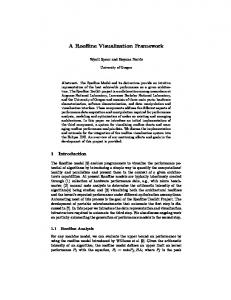
Figure 1: Simulation results on a three class benchmark data set using PCA and a global linear map optimizing the t-SNE cost function, respectively. The latter leads to a better separation due to its local nature, which can be formally evaluated using the measure of intrusion and extrusion on the resulting mapping. preservation of local structures formulated in the t-SNE objective rather than the preservation of global variances as used in PCA. A quantitative evaluation of the two mappings is also included in the lower right panel of Figure 1, based on the quality measure proposed by Lee and Verleysen (2008, 2009). Basically, it relies on k-intrusions and k-extrusions, which means it compares k-ary neighborhoods given in the original high-dimensional space with those occurring in the low-dimensional space. Intrusion refers to samples intruding a neighborhood in the embedding space, while extrusion counts the number of samples which are missing in the projected k-ary neighborhoods. The overall quality measure Q measures the percentage of data which is neither k-intrusive nor k-extrusive. In the optimal case all neighborhoods are exactly preserved which results in a value of Q = 1. B measures the percentage of k-intrusions minus the percentage of k-extrusions in the projection and therefore shows the tendency of the mapping method: techniques with negative values for B are characterized by extrusive behavior, while those with positive values tend to be more intrusive. Obviously, DiReduct shows a superior quality, in particular for small neighborhood ranges, since it preserves local structures of the data to a larger extent. Further, unlike PCA which displays a trend towards highly intrusive behavior, it is rather neutral in the mapping character, being mildly extrusive for medium values of k.
18
5 Local Linear t-SNE Mappings In this section we consider nonlinear mapping functions obtained by the principles outlined above. Again, we employ the t-SNE cost function. The functional form fW is chosen in two different ways: First, we consider fW given by a multilayer feedforward network as proposed by van der Maaten (2009). The update equations for a feedforward network can be derived from the t-SNE cost function and are similar to standard back-propagation, see (van der Maaten, 2009) for details. Second, we consider a locally linear projection which is based on local mappings obtained by prototype-based techniques such as neural gas in combination with local PCA or mixtures of probabilistic PCA (M¨oller and Hoffmann, 2004). The latter techniques provide a set of prototypes wk ∈ IRD , dividing the data space into k receptive fields, and corresponding local projections Ωk ∈ IRm×D with m ≤ D. We assume that locally linear projections of the data points are derived from one of these techniques: xi → pk (xi ) = Ωk (xi − wk )
(16)
with local matrices Ωk and prototypes wk . We assume furthermore Pthe existence of i responsibilities rik of the local mapping pk for data point x , where k rik = 1. In the following, we choose simple responsibilities based on the receptive fields: ( 1 if dist(xi , wk ) ≤ dist(xi , wj ) ∀k 6= j rik = (17) 0 otherwise More generally, a point x is associated with the responsibilities rk (x) in the same way. A global nonlinear mapping function combines these linear projections: X rk (Ak · pk (x) + ok ) , (18) fW : x → yb = k
using local linear projections Ak and local offsets ok to align the local pieces. The number of parameters W that have to be determined, depends on the number of local projections k and their dimension m. Usually, it is much smaller than the number of parameters when projecting all points y i directly. Hence, it is sufficient to consider a small part of the given training data only, in order to obtained a valid dimension reduction. We determine the parameters by a stochastic gradient descent based on the derivative of the t-SNE cost function: ∂qij ∂dE (b y i , ybj )2 ∂Et−SNE X ∂Et−SNE = · · ∂ok ∂qij ∂ok ∂dE (b y i , ybj )2 ij ς +1X (pij − qji ) = · (b y i − ybj )(rik − rjk ) i j 2 ς 1 + dE (b y , yb ) /ς ij
19
(19)
and ∂qij ∂dE (b y i , ybj )2 ∂Et−SNE X ∂Et−SNE = · · (20) i j 2 ∂Ak ∂q ∂A b ∂d (b y , y ) ij k E ij (pij − qji ) ς +1X = · (b y i − ybj )(rik pk (xi ) − rjk pk (xj )) i j 2 ς 1 + dE (b y , yb ) /ς ij assuming Euclidean distance in the projection space, as before. As an example, we show the results obtained on the UCI image segmentation data set. It consists of 7 classes and 2310 instances of 3×3 regions randomly drawn from 7 hand segmented outdoor images. Three of the 19 features were not taken into account, because they show no variance. We scaled the features by dividing with the maximal feature value in the data followed by PCA reducing the dimension to 10. For the locally linear projection, we run the Neural Gas algorithm (Martinetz and Schulten, 1991; Cottrell et al., 2006) with 14 prototypes to get a division of the data space into receptive fields. PCA was applied to every receptive field to define local transformations Ωk . Together with the respective prototypes wk this offers the corresponding data projections pk (xi ) (see Eq. (16)). The transformations Ak ∈ IR2×10 were set as rectangular matrices to perform the dimension reduction from 10 to 2 dimensions. The offsets ok are vectors in IR2 . The mapping parameters were initialized with small random values and a stochastic gradient descent was performed with 300 epochs and learning rate annealed from 0.3 to 0.01. The perplexity of t-SNE was set to 50. For the neural network embedding, we use parametric t-SNE with default parameters as provided in the implementation (given by van der Maaten, 2009). An optimum network architecture was picked varying the number of neurons from 50 to 2000 per hidden layer. The architecture is given by a [100 100 500 2]-layer neural network. The perplexity was optimized on the data and picked as 25. For comparison, we present the result of a powerful parametric dimensionality reduction technique, namely the generative topographic mapping (GTM) Bishop and Williams (1998). It obtains a prototype-based mapping by simultaneous clustering and topographic ordering while training. We use a 10 × 10 lattice for data visualization, and 3 × 3 base functions for the mapping of the latent space to the data space. Convergence after 20 epochs was observed. The results for a locally linear t-SNE mapping and parametric t-SNE in comparison to GTM are shown in Figure 2. In both cases, we used a subset of roughly ten percent for training, and we report the results of the mapping on training set and test set. Interestingly, as measured by the quality of the mapping, t-SNE in comparison with locally linear mapping is superior to a neural network based approach and the GTM. Since the data set is labeled, an evaluation of the projection in terms of the nearest neighbor classification error is also possible. The 5 nearest neighbor error for the whole preprocessed data after PCA to 10 dimensions is 0.054. After further dimension reduction this error increase due to the loss of information. For a locally linear mapping the 5-nearest neighbor error is 0.21 for the training set and 0.16 for the full data set, the corresponding projections are shown in the upper panel. The panels in the middle show the corresponding mappings achieved by parametric t-SNE (5 nearest neighbor error: 0.5 in training and 0.32 for the whole set, respectively). The bottom 20
DiReduct training set
DiReduct whole set grass path window cement foliage sky brickface
parametric t-SNE training set
parametric t-SNE whole set
GTM training set
GTM whole set
Quality on the training set 0.8
Quality on the whole set 0.8
Q
0.6
0.6
Q
DiReduct 0.4
DiReduct 0.4
parametric t-SNE
parametric t-SNE
GTM
GTM
0.2 0 -0.2
0.2 0
B 10
20 30 neighborhood k
40
50
-0.2
B 100
200 300 neighborhood k
400
500
Figure 2: Projection of the image segmentation data set using parametric t-SNE, GTM and DiReduct combining unsupervised clustering and the learning of a mapping. The result of the subsample used for training (left panels) as well as the full data set (right panels) are depicted. The intrusion/extrusion quality on the whole data set for all methods is shown in the bottom panel.
21
panel contains the evaluation of the mappings using the quality measure as proposed by Lee and Verleysen (2008, 2009). Interestingly, both functional forms show a good generalization ability in the sense that the error of the full data set resembles the error on the test set. However, the results of locally linear mappings are superior to a feedforward mapping in both cases.
6 Supervised dimensionality reduction mapping Mapping high-dimensional data to low-dimensions is connected to an information loss and, depending on the dimensionality reducing visualization technique, different data visualizations are derived. Since many methods such as t-SNE do not yield a unique solution, it can even happen that a data set is visualized in different ways with a single dimensionality reducing visualization technique in different runs. It can be argued (see e.g. van der Maaten and Hinton (2008)) that this effect is desirable since it mirrors different possible views of the given data, reflecting the ill-posedness of the problem. Auxiliary information in the form of class labels can be useful to shape the problem in such settings and to resolve (parts of) the inherent ambiguities. Aspects of the data should be included into the visualization which are of particular relevance for the given class labels, while aspects can be neglected if they are not so important for the given labeling. Thus, additional information, such as label information, can improve the results of dimension reduction by reducing possible “noise” in the data and keeping the essential information to discriminate the classes. This observation has led to the development of a variety of visualization techniques which take given labels into account. These methods still map the original data to lowdimensions, but they do so using the additional information. Examples for such methods include linear discriminant analysis and variations, supervised NeRV, supervised Isomap, multiple relational embedding, etc. (Venna et al., 2010a), for example, give a recent overview and compare various methods for supervised data visualization. Here, we essentially repeat the experiments as proposed in Venna et al. (2010a) to demonstrate the suitability of our general method to incorporate auxiliary information into the data visualization. In this section we show some examples of the proposed method based on the t-SNE cost function, employing supervised local linear projections pk (xi ) (Eq. (16)). Here, the parameters Ωk and wk are acquired by a supervised prototype based classifier, limited rank matrix learning vector quantization (LiRaM LVQ; Bunte et al., 2010; Schneider et al., 2009). We compare the results to alternative state of the art techniques on the three data sets mimicking the experiments by Venna et al. (2010a): • The letter recognition data set (referred to as Letter in the following) from the UCI Machine Learning Repository (Asuncion et al., 1998). It is a 16-dimensional data set of 4 × 4 images of the 26 capital letters of the alphabet. These 26 classes base on 20 different distorted fonts. In total, 20000 data points are given. • The Phoneme data set taken from LVQ-PAK (Kohonen et al., 1996) consists of 20-dimensional feature vectors representing phoneme samples stemming from 13 different classes. 22
• The Landsat satellite data set is contained in the UCI Machine Learning Repository. Each of the 6435 36-dimensional vectors corresponds to a 3 × 3 satellite image measured in four spectral bands. The six classes indicate the terrain type in the image: red soil, cotton crop, grey soil, damp grey soil, soil with vegetation stubble, and very damp grey soil. For these data sets, we consider a projection to two dimensions by means of a locally linear function, as before, characterized by the functional form Eq. (18). Unlike the previous setting, this form is biased towards the given class information, because the local projections pk are determined by means of a supervised prototype-based projection method: We used LiRaM LVQ with the rank of the matrices limited to 10 (for Letter and Phoneme) and 30 (for Landsat), respectively. Based on this setting, the offsets ok are determined by means of the prototypes, and the initial projections Ωk are given directly by the square root of the matrices obtained by LiRaM LVQ to obtain good class separation. Correspondingly, the parameter matrices Ak map from 10 or 30 dimensions to two dimensions in this case. The supervised training of the initial functional form of the mapping function, Eq. (18), by means of LiRaM LVQ as well as the (unsupervised) training of the free parameters of the mapping function takes place using only a small subset of the full data set (7%-18%) while the evaluation takes into account the full data set. The goal of supervised dimension reduction is the preservation of classification performance, and, is hence, quite different to classical unsupervised dimension reduction. In consequence, the quality assessment of the final embedding should be done differently. Here, following the approach of Venna et al. (2010a), we measure the 5-nearest neighbor classification error (5NN error) of the resulting visualizations achieved in a 10-fold cross validation scheme. We compare the result obtained by locally linear projection based on the t-SNE cost function and a functional form biased by a discriminative prototype based classifier as specified above to several state-of-the-art supervised nonlinear embedding methods taken from Venna et al. (2010a): • Supervised NeRV (SNeRV; Venna et al., 2010a) which uses input distances dX (xi , xj ) induced by the Fisher information from a non-parametric supervised classifier. • Multiple relational embedding (MRE; Memisevic and Hinton, 2005) which is an extension of SNE accommodating additional characteristics of the data space or subspaces provided as similarity relations priorly known to the user. • Colored maximum variance unfolding (Song et al., 2008b) is an extension of the unsupervised maximum variance unfolding. It is also called maximum unfolding via Hilbert-Schmidt independence criterion (MUHSIC), because it maximizes the dependency between the embedding coordinates and the labels. • Supervised Isomap (S-Isomap; Geng et al., 2005) is an extension of unsupervised Isomap extending distances to incorporate label information in an ad hoc manner. • Parametric embedding (PE; Iwata et al., 2007) aims at the preservation of the topology of the original data by minimizing a sum of Kullback-Leibler divergences between a Gaussian mixture model in the original and embedding space. 23
• Neighborhood component analysis (NCA; Goldberger et al., 2004) adapts a metric by finding a linear transformation of the original data such that the average leave-one-out k-nearest neighbor classification performance is maximized in the transformed space. Note that these methods constitute representative supervised visualization techniques which enrich dimensionality reduction by incorporating given label information in various forms. 1
Original data DiReduct Map (training)
0.9
DiReduct Map (all) SNeRV l=0.1
5NN classification error rate
0.8
SNeRV l=0.3 PE
0.7
S-Isomap MUHSIC
0.6
MRE NCA
0.5 0.4 0.3 0.2 0.1 0
Letter
Phoneme
Landsat
Figure 3: 5-nearest neighbor errors of all methods on the three data sets. The error rates of the nearest neighbor classification (using squared Euclidean distance) on the whole original high-dimensional data set and after dimension reduction with the different methods are shown in Figure 3. In contrast to our method, the other techniques were evaluated using only a small subset of the data sets (only 1500 sampled points), because they are based on the embedding of single points. For our approach, we train on a subsample of 7% only, but also report the results of the full data set obtained by the explicit mapping. Note that the classification error obtained by an explicit mapping biased according to auxiliary information is smaller than the alternatives for all three data sets. It is remarkable, that the error in the reduced space is also comparable to the error on the high-dimensional data for most data sets. For the Phoneme data set the supervised dimension reduction even leads to a better separation of the classes than in the original space. Hence the proposed method displays excellent generalization, this way offering an efficient technique to deal with large data sets by inferring a mapping on a small subset only. Example visualizations of the proposed method are displayed in Figure 4. A clear class structure is visible especially for the data sets Letter and Phoneme. Interestingly, the Letter clusters arrange in a quite intuitive way: “O”, “Q”, 24
Letter (training set) M MM M M M M M M M M M M MM M M M M M M M M M M M MM M M M D
Letter (whole set)
M
prototypes UUU U U LU U U U U U U U U U U UU U U O KN N QQQ N N N D OO Q Q Q QO Q Q ND N Q O N N N NJ O O Q O Q Q NF N Q N Q N N N N Q Q O N N Q O N N Q O O O O O Q Q O Q O O Q O N O O OO Q ON Q O Q O QQ O H Q O NN O O HO J Q J R HKH H B R G G G C H H HHH H RR G H R R KR R R H HH H H H R G R G G G G KR HH H GG R R H RRK R R R R H GG R KK RR G GQ G D G R G H RR Y H G H G R H G R G G EK HH R G G G RR K D K K K R R K T K K K K K KK K KK K K K K K K K HB B K BB BBB B B E B B B C E B EE ST CC B B C C R BX C C B B C XEE B C C BTB C C C C XXXX X C CC K C C C B C IBB U C ES EE E EE FBXX EEE E E X E CC X E X G X DD CCC XX E X D X E X X E E X D E CCC N XX X B D G E VG XX E D F XX X E D DD D E X D X X D D D D D D X D X D D D X D X D D D D DDD D O D T I D D TT LVT T TT TTTT T TT T SSZ S T T J SSSSS T T T SS TV S T LLL L SS T TTT S S S S S SS S S A S A SS A A L A AG SS AA A A A L A L LL A L A A LL A LLL L A A A A L A L A L LLLLL L A Y Y A Y Y VY Y Y Y Y Y Y Y F F Y F Y Y Y Y F FF YY FF FFFF H B YYY F FF ZZIZ Y YY FF ZZZZZ P ZZZ Z F FF Z FFFF P P ZZ ZZ ZZZ P ZZ P P G P P ZZ P I P P J FPPPP P P V P V P IIII P ZZZ V P S V P P PPP V VV V PP V V P V V V PPP P I IIIIIII V V IIIIIII V V V V V V V I A J JJJJ JJJJ J JJ JJ JJ JJJ JJJJJJJ I W W W W W WW W W J W W W W W W U WW W W VW W W W W N W W W W W W WW W
M MM U M M M M M M M M M MM M M M WM M M M M M M M M M M M W M M M NM M M M M M M M M M M M U M M M M M M M M MM M M M M MM MM U M M M M M K MM M M M M M W M M M U MM M N M M M M M M M M M KU M M M M M M U U M M W M M U U N MM M M M M M N M M J W U M M M M G M M M U M K U U MM MMM M A M U U M A M U U M U U M M D M A H H U A M D M M UU U M M U M M D M W A U M M U X U M K K Y M U U W M H U M A W X NNN LJU X Y U U M X A U R M C U U A A M U U U M D U A U U DM X X J U U K O M K M W U U C U U U K U K X W X U G U O R A U U U UU A U U UU K X U C H U U U U A L UU O U C O U R X U Y A UU K U U U U U D U N UU H X U H Y N J U O J U MN U UU A N X A U A UU U O O X N U O O U U U A W UU UU U U U A O U U U G A H U UU U U C U H O G C U X Y Y A N A U C O U A U O O U D U U U U S W G X A C UU A H U U U U U O U U A U U U O U A UA D H CU J S U C U N U U K U U Y Y U A U H A Y U K O W U K G N N D K O K H D B B Q A U G G M N N O Y GG QQQ U M UN F O N N Y G K Q K N Q W N N N Q O O N D O R H O L N U R O O W O O J O V K N K P O N K G F K H O D P S G U Q Q B U Q R O Q Q F E J N I N G N Q N G O N O O N O I O Q N W N G K O D Q V O C W B O Q H N N R Q O R O O U R N Q M N Q N N O K N Q O Q O O D N N D O G Q Q N Q M K D N S Q O S S D D N N NN Q A E S Q NN N O S N N Q Q K G O Q R D N Q NN R V P P N Q Q O O O N N N Q N L F N N W Q O Q G G K N J O N H V G G D N Q R K X N N N O N O R O U W P O P Q O O O N M O O Q N Y E O Q O Q U QQ O O O Q Q N Q O G U O SO QQ N H K O U Q R L Q N N X J N K Q Q Y O O Q J N P Q K V V F Q Q Q N P D O K W D G N Q Q W N J Q O H M N Q Q N O A Y N C D Q Q N J L F W SO H Q N N O M O P Q J Q N O N G O S N J Q U O W O Q N L F U C Q Q N QQ O N H Q U M G M Q O N N N D O Q F D N U Q N Q R V O J Y Q O O D OO O D N C O L O E O Q L O Q QQ Q R S N N O N N G O R O Q N D O Q Q V O D N QQ Q J C O O W N X Q Q Q N U O O Q G U P N G N Q N FF N NN O K O Q Q W R OO J O D P R F Q C O Q N O Q O Q O N O N O Q N Q N Q Q K N K A U V O Q W Q Q N Q W N F W Q V N N O N P L O O B R Q L Q N Q U O D O K O U O N F W N Q P V L N O N H N E Q N Q J S F S O Q N N J Q W Q G O G Q U M O NN O L O O P W H O W K G O O X G Q N L Q F N U O O O F Q D Q Q H Q E W O N N C M Q Q M G H M N F L Z O O N O O N C L O W O W Q J N N P N R Q W P O N O W N X C H L Q H K O O A N C O O V N Q N J C Q O O O O L O O N U O H G Q H Z Q UN O Q AU CZC O L G Z OO P JSRH G C O C K K O Q G P K C N C O FLU K Q Q N NM T K MM Y J Q R O N J K Y X J K T K R O O R O C H O H H HG R R O R J R T J H RR O H R F H B J A K H O K R J T H O T M O K J J J Q B O M I K R J H P R G R R R C H O H R O G G V T O R I R H G R R G H K H K R H O K H G H H H J Y N KHY R T S X K K K K K V H JB H O Y C G G R Y C R C G H U R H H S C O O X H R R F K G K J R E J Y H R H G J O G H H I H G H V K C H H G HH G H X R R R K R R G G H H R O O G R Y HH R K T X Q R H B N X R R H I K R H Y M R K O O B I K H R G A T H H H H W K G G N G C R R R R O D B Y H W B Q K G Q H G H K H H Q Q O U H K R K Y C H H T H Q Y Y G G L G K D X I G V G G D G S N K X R A V G G H C K F N I R C G K K R G R C G K H R H D R R R R H G T H H G K R H K H H G W S H L H H Q H U K R M N HH R R H D R B B K R I B G R G K K A R V H H R Q K H H R H K G L H O G G R R K H H Q K G G P K F J A C HH G G IK Q G H IR M D R R Y D O C K Y K B R GG H G R Y E H RR E P R IK C M G U G K Q G Q Q G H H G Q B G GG R H E G B A O D H G R P T T R G B FH K G K R G T B R H R R C H IH HS Y H GG R H L IH K YY T O H D K G M R R G G IR G H G G H R G P M LK C H K R H H B H H R T T G H GG H H G R Y C G G G R G C D Q K B R R H D H K H D X G K R R H G Y T KN K R C Q G G G K K R K U R E G E G Q G G H L E IX R R M T B H R O G R C R G R D T K C D ID H G K K H H H E P T ID H H R G N Q K H R B G T H G G H H K K R IRR R R L L P H K X G R K P R T G T F G K R H B ID H E G M H KK K H U R E E B X K R R G G N G K P B T R G H Q K K R R E K S IB X T G Q S B X T T M B X C G G Q L H H R F T E Q K H H L K N R F L P X K T S E N G K K R H D Q K C H K P P K X G K Q KK Y O K N K M G IB E X K G L PM E K K E X R X KK R K K O K R H K R KK K R R C K K B K K R L P K K B K T K N H R X K K K K K K K X K K C B K X KK K K K K K K K K K K X K R R B X R X KK K K X R G N BB K K K R H H K X X K K X K K X I B K H B X K T B H H K X K X K K U B K W B B K L T R K B H K H R X B K B R D K K R H R H K K K B X B G K E B B B R X B B B R K X E C H E B G X B RK C G G T K KXX B K H E B R U D E B U E G M O E D B R D E B T B EE B B C H E B B C E W B B T D B E B C E E U U L R S B C R S EE C K B B G E P B BB A E E BB B B XX R H S R G L B A G C E G M BB U B B V S X X H KK E C V O D B E C R C O H C O Q B XX B BB B C U S B B R C B Q H L S B G C E E C C S T B E S DD DV T B U C V B B B B T B Q G F B U C F C G C C G B B K H G C S R G C Y S B S B G P C E E B E G T G F E M B G C S F BB X H K Y Y F P E E C V E F C O F C BB M E C T X Y V V B IL R LEE H H X B B CC Q L T Q H B S B A E B N X H CC S T T C T B B C CC E Z C C B C S F C C C S B B Q CC L D S L C T H N R F C E S Q C C B C B M G C C G D F X E Z C E B S E X V B S S E Q F L S X R C M L F E B L V L E P C B B Q F L S B C C E T B K G V V H E Q C Z CC L E C Q P C E BB B K H K CC E T B X CC CC IZ C CC G S S S X Z F U G Q X C E E C X B X H Z C C B H C EE CC E G X E C C Q H F K ID C S X E IV V C B E D X K R U E Z C B S C E K Z L D U C FY Z C U F C E E L G Z C Y CC D X G E K G T B X HK F C CC IIP C C H D T B B IH Y E B Q L C L T B X C E D E Q W X N X X X E D K EE E E C G F K K LL G D X Z C W EE S M X B C Y C E D G IE L E X E C ID C C L C L B J X L EE C K T B R E H E E E X B X R G R EE T E C E D X H E K F D X E G G VG E E E E F K G J C X K C E R B H C C S B R N D E F X H ID C L IX R L C X R L X IX K E F D X G C CC X K E F D B K C EE F G D H E U K F X T X R C A CC C D B F E X B C K D K K Q X K G H J EE ZZU FC DD D X K A V E C X IF T T C E K F X E G X C F G E E F B C E E B X G S O XXX E F C E T E Q K E L D E E C D E X K XX F L H X Q G G G C IDDW E G T D S X K K E IS XX H D C T D D F X U T D X X D X Z J C J X O H E O D B G G Q X J T D X X K C Y E XX N D F B F X C E C F H X K G XX D X F X N G R F D X X CC D X H D K U R Y X H D S IID X K X C M IF B X IG C D B C G G G ID D B G A Q C M H D ID H D W X Z V E E H R X C Y E M F G G E EE D G X D D G X M E E D X DD C D XX E X K K X P D D D K J E F D K S G J D X XX X Y N E K J A C O D E D X X C K L O D DD X K D X E D XXX R A D X E H W IS R U S X G T U D IE LT U D IK R J L X X E T B Q D FG H X XX X F K P IJ B X X P D T R X P O D H D S D D D I D F D Q X D K U B K P F DD D B X H A U X I I D K D J Q E D H B D H D D B B S M X B D X X R P R L B D T P H D X I J D X K J X B X R D I G H M X G J DD H DD H B S D L X D O R X D X N D H J D L F S S DD M S I D B H D O K Y O H D H T D X G D D X X Y H O O L L D F S B X X M H X X F F R R D Z D D X I Z D T B X U H H L D D Z F T T B N I X J R D D F S T R U V DD H O W H H U U A F H BB R H D S Y S T F T K R T IY H D C L R X Y ZS H T H D T T D T M T R A F T T JJX F HD T B D U Y D K N Y L L T D S U N U Z T B D Z V T T L Y K S Z U T T T L S Z O U D H S Y B C T T E Y Y T S B F SS S TTT T S T T S U S H U T T B R Z V T T TT T R Z N E Z Y T D S Z T T D F T S T T F X V TT B S S LL S A Y Z L E TT F TT T R Q M T T S H V T T Z Y TT Y D TT S Y T S S J F B F T F E S B D IS E T Z T H X S X T S T X R Z TT T S F S A T Z S TT X Z F T F T T TT S T T S T X S S Y T C S S S S T C S T IS T B E T S L T S T B B V T E S A L S Y H X T S A Z F S G E IP LS T Y L S A LSS S S T T S IS T S S A A Y S S X F IJJX P IT A T S B S S X Z T S X L T E SS S X J V S S S A V L T Y T P S T S A S S A L Y H LL H F LL B T R L A F B AA F F A S L Y L L T L LC T B R T T J J J X T E S T SS G X Q C S A A Q S F S U S IZ IX Y S S S Q A L L TT S F K L G A F S S SA IS A A Y T F L S T S S S K A Z T X X Y F A A Y L F A SS A S G AA JJ T L F L L S J A L K S A L S B IS AA L L X H J A IL S S S ISS L T S H A Z F T J Z L L B A L S X LL Q L P F H T S S AA J A S S S H X AA Y D S AA A A A V S A P A L A H LL T A S H L L L A S A LL L S L T A A S A A A L A K A A L L L A L S L L S S A A L Y LL L S JF AA L Q Z S AA S FT LL D A Y Z T H G S S H LL S L A LL H A S Q A LL S SY G J S Q A Q Q R A I A A A L L T SSM JA L T S L L L L A A L L A L Q A Y S A L A G A R L L L L T B IQ A L J H S JL A J J G Q F L A P L Y LL L F H L Q J J R H M L Q A Y M A Y P L L S L B N A R A IA L A P A AA A L JY M L L J Y J A Y B A Y Y S Y J Q Q R SCF Y L A A Y Y F M Y L L T A G A Y M A M A Y Y Y Y J Y A A L L H P A L T F G Y F Y A Y S X Y P A L Y H A Y Y Y F HN I G Y YY G S T M B A A YY Z F G F Y Y A YY Y T M L A Y M Y X Y L F Y Y Y Y M Y S Y Y V L F Y YY Y Y Y Y F G T Y F C G Y Y S G Y Y G I Y F Y Y S F Y Y Y Y F Y Y Y Y F S M F G YY V G Y S YY Y Y M G E E L F YY Y F Y P Y D F J YY F Y E E P Y M IQ F G Q Y Y T F F T Y Y F YY Y Y Y E F F F F F Z Z Y S P Q F L S I Y T F Y E S X Y F Y F F E Y T X X Y Y F I J Y F Q G E Y Y T P V F Z FF F I F Y F X P L H H P Z Y Y Y P Z J Z V V Y Y V D F F Y Q L F Y Y Z Z F P Y F F I J Y Y Y T FF F F S T Y F Y Y Y Y S F J P Y F F P B Z Y F F T FF F F F F Z Z FF FF F F T T Z L B Z F Y Y Y Q O Q Z F P Z F Z E Y P F E X IO Y T Z T Z E P Y YY F Y Q X Y B F E F F F F A P FF S Y T G Y Z FF J Z Z Y L B E S F P Y P Z F F F I Y F F F S P Y Y V E Z F F Y ZZ F Z Z F P V Z E S I Y Z V F D P S F F P Z T F J Y Z F F P I H Z Z F P P Q Q I G F P I H Z Z F Q X P S S I YY F X Z X X F G Z Z T P S Z Z E T B X FF F Z P Z O I E F Z F E B F P D Z Z S I Z YYA Y Z P B J J F P Q Y F B F P Z F Q Z F D T P Z S F A Z P P F Z P F Z Z ZZZ P F Z Z E F S F D I Z P S Z Y P F S S Z P P P Z E S X Z ZZ Z Z F R Z S J P P T P Y FX N R I I Z G PY Y P D S IS P ZZ ZZ V P S F P X J JG S Z IE ZZ P S P P B H V Y F P Q J Q Z Z ZZ S P Z Y Z P G Z L F X U Z Z ZZ P E F Y S F F P Z T Z Z D P Z Q Z P Z Y S F P S Z Z FIL B X Z S F IIF Z O Y P S P IIX G P Q PP P P V P P FIJF O P P B Z P P V T V Z VV P P V Z P F ZZZ Z Z G S P V Z Q A J O K A Z V Z Z S IF F Z Z F S A V Z IIIIIIIIIII B V D A Y P Z D P P F Y P P P Z V Y P H P Y E P S P P P Z F F P P P Q V F Q P V P P D III V Y PP P P VV P F S V P PP G Z N ZZ V P Y Z Z V Y Z VV PP V P O P Y S V P P P K T K PP S F K V P V V IIIIIIIIIIJ V P O A P P IIII Y V V P A V P JJZ F P P Y V V Y V ZQ G P PP V V P V P II ZS P P P Z V FPP V IIIIIIIJ V Y P Z G V F P II V P IS V VV P P IIZ P P IIJ P T V V F V O IIJ F Q P V V V IIIP IIIP P G P Q G P Y V W V P P IJP IIIP V V IIIJ G V V P PP VV W Y P P Y H G VVV V V V V V V P V VV G P B V Y Y F P V IIIIIIIIIIIIIII G V V P P IIII J P T V V P V V P V Y F V V V V V V Y Y V V Y P YPP V V ZZZ G VV V V VV V VY V V P P S V V V V V G Y Y T G V G V V P P P II H H IJIZIS P IP F N IS IJ I S K J Y VA J JJ JJ J JJ J JJJ J J J J J J JJ JJJJJJ X JJJ J J JJ JJIJ J JJ W J J J W J J J W J J J J JJ JJ J J J J J J J J J JJ W JJ J X J W W J J J J J J J J W J J F X J J J J OW I J J J W W W J J X J W JIXJ W W JJS S W JP W JJ S JIIJP IIJ W W W W W W JJJJ W W W W P W W W SJ S W O W W W M W W W W M W W W M JJ W J W SS W W W U W Q V M W W W S W W R V U JJIFII W W W W W W W WW W W W O W W U U WW W K W W M W M G M M V W W W W V W WW W M M Q WW U M W W N W W WW U O W W WW W G O W M Q R V W M W G W W W W W V K W N MM M W R W P V M V W W U O M M W W M H K W W W W U W W W A M M V G M K M W W V W F W W F V W U W R W W F W M U W A A M M U V W C U W AM KUUW
Phoneme (training set)
Phoneme (whole set)
1 2 3 4 5 6 7 8 9 10 11 12 13 Landsat (training set)
Landsat (whole set)
1 2 3 4 5 6
Figure 4: Example visualizations of the data sets in two dimensions. “G” and “C” stay close together, so do “M”, “N” and “H”. The qualitative characteristic of the projections is the same for the training data and the full data sets, displaying the excellent generalization ability of the proposed method.
25
7 Generalization Ability and Computational Complexity The introduction of a general view on dimension reduction as cost optimization extends the existing techniques to large data sets by subsampling. A mapping function fW based on a small data subset is obtained which extends the embedding to arbitrary points x coming from the same distribution as the training samples. In this context it is of particular interest if the procedure can be substantiated by mathematical guarantees concerning its generalization ability. We are interested in the question if a mapping achieves good quality on arbitrary data assuming it showed satisfactory embeddings on a finite subset, which has been used to determine the mapping parameters. A formal evaluation measure of dimensionality reduction has been proposed by Lee and Verleysen (2009); Venna et al. (2010a), based on the measurement of local neighborhoods and their preservation while projecting the data. Since these measures rely on a finite number of neighbors, they are not directly suited as evaluation measures for arbitrary data distributions in IRN . Furthermore, restrictions on the applicability of these quality measures to evaluate clusterings, have been published recently by Mokbel et al. (2010).
A possible formalization As pointed out by Lee and Verleysen (2009) one alternative objective of dimension reduction is to preserve the available information as much as possible – this objective is usually hardly used to evaluate non-parametric dimensionality reduction because it cannot be evaluated due to the lack of an explicit mapping. Given an explicit mapping, however, it can act as a valid evaluation measure: the error of a dimensionality reduction mapping f is defined as Z E(P ) := kx − f −1 (f (x))k2 P (x) dx (21) X
where P defines the probability measure according to which the data x are distributed in X and f −1 denotes an approximate inverse mapping of f ; an exact inverse might not exist in general, but local inversion is usually possible apart from sets of measure 0. In practice the full data manifold is not available such that this objective can neither be evaluated nor optimized given a finite data set. Rather, the empirical error X bn (x) := 1 E kxi − f −1 (f (xi ))k2 n i
(22)
can be computed based on given data samples xi . A dimension reduction mapping bn (x) is representative for the shows good generalization ability iff the empirical error E true error E(P ). If the form of f is fixed prior to training, we can specify a function class F with f ∈ F independently of the given training set. Assuming representative vectors xi are chosen independently and identically distributed according to P the question is whether the empirical error allows to limit the real error E(P ) we are interested in. As usual, 26
bounds should hold simultaneously for all possible functions in F to circumvent the problem that the function f is chosen according to the given training data. This setting can be captured in the classical framework of computational learning theory, as specified e.g. by Bartlett and Mendelson (2003). We can adapt Theorem 8 of (Bartlett and Mendelson, 2003) to our setting: We assume that the norm of the input data is limited to the unit ball. Possibly, prior normalization is necessary, which would be mirrored by corresponding constants in the bounds. We consider the loss function L : X × X → [0, 1]
,
(xi , xj ) → kxi − xj k2 .
(23)
Then, as reported by Bartlett and Mendelson (2003) (Theorem 8), assuming i.i.d. data according to P , for any confidence δ ∈ (0, 1) and every f ∈ F the relation r bn (x) + Rn (LF ) + 8 ln(2/δ) E(P ) ≤ E (24) n holds with probability at least 1 − δ where LF := {x 7→ L(f −1 (f (x)), x) | f ∈ F}
(25)
and Rn refers to the so-called Rademacher complexity of the function class. The Rademacher complexity constitutes a quantity which, similar to the Vapnik Chervonenkis dimension, estimates the capacity of a given function class, see (Bartlett and Mendelson, 2003). The Rademacher complexity of many function classes (such as piecewise constant, piecewise linear functions with a fixed number of pieces, or polynomials of fixed degree) can be limited by a term which scales as n−1/2 . See (Bartlett and Mendelson, 2003) for structural results and explicit bounds for e.g. linear functions, and e.g. (Schneider et al., 2009) for explicit bounds on piecewise constant functions as induced by prototype based clustering. This result implies that the generalization ability of dimensionality reduction mappings as considered above can be guaranteed in principle since the Gaussian complexity of the class LF can be limited in our settings. It remains a subject of future research to find explicit good bounds.
Complexity Assume a set X of points is given. Most dimensionality reduction techniques are computationally quite demanding due to the form if the overall costs (9): since, usually, the characteristics map sequences of points to sequences of real values of the same length, the computation of (9) is at least O(|X|2 ). This is infeasible for large X. Out-of-sample extensions by means of an implicit mapping depend on a subset X0 ⊂ X only. If the principle as derived in this paper is used, the corresponding complexity is given by O(|X0 |2 + |X0 | · |X|), since only the subset X0 is mapped using the original method, afterwards, all remaining points are mapped by separately optimizing the costs of one x ∈ X regarding their relation to X0 , the latter being O(|X0 |) for every x. Thus, this approach substantially reduces the effort depending on the size of X0 , but it does not easily allow a way to control the form of the mapping, or to integrate prior label information. By choosing an explicit functional form, the complexity is further reduced to O((|X0 | · |W |)2 + |W | · |X|), assuming an effort O(|W |) to evaluate fW . Since, usually, |X| � |X0 | � |W |, this constitutes a further considerable reduction of the time required to map all points. 27
8 Conclusion In this contribution we reformulated dimension reduction as an optimization problem based on structural characteristics. As a consequence many popular nonparametric dimension reduction techniques can simultaneously be extended to learn an explicit mapping function. The optimization of a parametrized mapping function for dimension reduction is beneficial in several ways: large data sets can be dealt with because the mapping function can be learned on a small random subset of the data. Furthermore this framework allows us to consider the generalization ability of dimension reduction since an explicit cost function is available in terms of the reconstruction error. Interestingly, bounds as derived in the context of computational learning theory can be transferred to this setting. We showed the suitability of the approach based on the integration of global linear and locally linear projections into the t-SNE dimension reduction method on different data sets. Furthermore we show the integration of auxiliary (e.g. class) information into the framework. The proposed general framework is very flexible and can be combined with every possible form of the mapping function. The investigation of alternative dimension reduction mappings based on other cost functions and other functional forms of the mapping, as well as the derivation of explicit bounds on its generalization ability will be the subject of future work. At present, the settings have been restricted to Euclidean data only due to the form of the mapping fW . Naturally, more general forms could be considered which can take more complex, non-Euclidean data as inputs, such as mappings which are based on general dissimilarity characterization of data. Since it is not possible to embed such data in any Euclidean vector space, possibly qualitatively different results could occur. A corresponding investigation is the subject of future research.
Acknowledgments This work was supported by the ”Nederlandse organisatie voor Wetenschappelijke Onderzoek (NWO)“ under project code 612.066.620 and by the ”German Science Foundation (DFG)“ under grant number HA-2719/4-1. Moreover, financial support from the Cluster of Excellence 277 Cognitive Interaction Technology funded in the framework of the German Excellence Initiative is gratefully acknowledged.
References Asuncion, A., Newman, D. J., Hettich, S., Blake, C. L., and Merz, C. J. (1998). UCI repository of machine learning databases. http://archive.ics.uci.edu/ml/. Bae, S.-H., Choi, J. Y., Qiu, J., and Fox, G. C. (2010). Dimension reduction and visualization of large high-dimensional data via interpolation. In Proceedings of the 19th ACM International Symposium on High Performance Distributed Computing, HPDC ’10, pages 203–214, New York, NY, USA. ACM.
28
Bartlett, P. L. and Mendelson, S. (2003). Rademacher and Gaussian complexities: risk bounds and structural results. Journal of Machine Learning Research, 3:463–482. Baudat, G. and Anouar, F. (2000). Generalized discriminant analysis using a kernel approach. Neural Computation, 12:2385–2404. Belkin, M. and Niyogi., P. (2003). Laplacian eigenmaps for dimensionality reduction and data representation. Neural Computation, 15:1373–15396. Bishop, C. (2007). Pattern Recognition and Machine Learning. Springer. Bishop, C. M. and Williams, C. K. I. (1998). GTM: The generative topographic mapping. Neural Computation, 10:215–234. Brand, M. (2003). Charting a manifold. Technical Report 15, Mitsubishi Electric Research Laboratories (MERL). Bunte, K., Hammer, B., Wism¨uller, A., and Biehl, M. (2010). Adaptive local dissimilarity measures for discriminative dimension reduction of labeled data. Neurocomputing, 73(7-9):1074–1092. ´ (2010). The elastic embedding algorithm for dimensionality Carreira-Perpi˜na´ n, M. A. reduction. In 27th Int. Conf. Machine Learning (ICML 2010), pages 167–174. Cottrell, M., Hammer, B., Hasenfuss, A., and Villmann, T. (2006). Batch and median neural gas. Neural Networks, 19(6-7):762–771. Geng, X., Zhan, D.-C., and Zhou, Z.-H. (2005). Supervised nonlinear dimensionality reduction for visualization and classification. In IEEE Transactions on Systems, Man, and Cybernetics–Part B: Cybernetics, volume 35, pages 1098–1107. Goldberger, J., Roweis, S., Hinton, G., and Salakhutdinov, R. (2004). Neighbourhood components analysis. In Saul, L. K., Weiss, Y., and Bottou, L., editors, Advances in Neural Information Processing Systems 17, pages 513–520. MIT Press. Guyon, I. and Elisseeff, A. (2003). An introduction to variable and feature selection. Journal of Machine Learning Research, 3:1157–1182. He, X., Cai, D., Yan, S., and Zhang, H.-J. (2005). Neighborhood preserving embedding. In Computer Vision, 2005. ICCV 2005. Tenth IEEE International Conference on, volume 2, pages 1208 –1213 Vol. 2. Hinton, G. and Roweis, S. (2003). Stochastic neighbor embedding. In Advances in Neural Information Processing Systems 15, pages 833–840. MIT Press. Iwata, T., Saito, K., Ueda, N., Stromsten, S., Griffiths, T. L., and Tenenbaum, J. B. (2007). Parametric embedding for class visualization. Neural Computation 19, pages 2536–2556.
29
Kaski, S., Sinkkonen, J., and Peltonen, J. (2001). Bankruptcy analysis with selforganizing maps in learning metrics. IEEE Transactions on Neural Networks, 12:936–947. Keim, D. A., Mansmann, F., Schneidewind, J., Thomas, J., and Ziegler, H. (2008). Visual analytics: Scope and challenges. In Simoff, S., Boehlen, M. H., and Mazeika, A., editors, Visual Data Mining: Theory, Techniques and Tools for Visual Analytics. Springer. Lecture Notes in Computer Science (LNCS). Kohonen, T. (1995). Self-organizing Maps. Springer. Kohonen, T., Hynninen, J., Kangas, J., Laaksonen, J., and Torkkola, K. (1996). LVQ PAK: The learning vector quantization program package. Technical Report A30, Helsinki University of Technology, FIN-02150 Espoo, Finland. Lee, J. and Verleysen, M. (2007). Nonlinear dimensionality reduction. Springer, 1st edition. Lee, J. A. and Verleysen, M. (2008). Rank-based quality assessment of nonlinear dimensionality reduction. In 16th European Symposium on Artificial Neural Networks (ESANN), pages 49–54, Bruges, Belgium. Lee, J. A. and Verleysen, M. (2009). Quality assessment of dimensionality reduction: Rank-based criteria. Neurocomput., 72(7-9):1431–1443. Ma, B., Qu, H., and Wong, H. (2007). Kernel clustering-based discriminant analysis. Pattern Recognition, 40(1):324–327. Martinetz, T. and Schulten, K. (1991). A ”Neural-Gas” Network Learns Topologies. Artificial Neural Networks, I:397–402. Memisevic, R. and Hinton, G. (2005). Multiple relational embedding. In Saul, L. K., Weiss, Y., and Bottou, L., editors, Advances in Neural Information Processing Systems 17, pages 913–920. MIT Press, Cambridge, MA. Mokbel, B., Gisbrecht, A., and Hammer, B. (2010). On the effect of clustering on quality assessment measures for dimensionality reduction. In Neural Information Processing Systems workshop on Challenges of Data Visualization. M¨oller, R. and Hoffmann, H. (2004). An extension of neural gas to local PCA. Neurocomputing, 62(305-326). Peltonen, J., Klami, A., and Kaski, S. (2004). Improved learning of riemannian metrics for exploratory analysis. Neural Networks, 17:1087–1100. Roweis, S. T. and Saul, L. K. (2000). Nonlinear Dimensionality Reduction by Locally Linear Embedding. Science, 290(5500):2323–2326. Sammon, J. W. (1969). A Nonlinear Mapping for Data Structure Analysis. IEEE Transactions on Computers, C-18(5). 30
Schneider, P., Biehl, M., and Hammer, B. (2009). Adaptive relevance matrices in learning vector quantization. Neural Computation, 21(12):3532–3561. Song, L., Smola, A. J., Borgwardt, K. M., and Gretton, A. (2008a). Colored maximum variance unfolding. In Platt, J. C., Koller, D., Singer, Y., and Roweis, S. T., editors, Neural Information Processing Systems. MIT Press. Song, L., Smola, A. J., Borgwardt, K. M., and Gretton, A. (2008b). Colored maximum variance unfolding. In Platt, J., Koller, D., Singer, Y., and Roweis, S., editors, Advances in Neural Information Processing Systems 20. MIT Press, Cambridge, MA. Suykens, J. A. K. (2008). Data visualization and dimensionality reduction using kernel maps with a reference point. IEEE Transactions on Neural Networks, 19(9):1501 –1517. Teh, Y. W. and Roweis, S. (2003). Automatic alignment of local representations. In Advances in Neural Information Processing Systems 15, pages 841–848. MIT Press. Tenenbaum, J. B., Silva, V. d., and Langford, J. C. (2000). A Global Geometric Framework for Nonlinear Dimensionality Reduction. Science, 290(5500):2319–2323. Torgerson, W. (1952). Multidimensional scaling, I: Theory and method. Psychometrika, 17:401–419. van der Maaten, L. J. P. (2009). Learning a parametric embedding by preserving local structure. In Proceedings of the 12th International Conference on Artificial Intelligence and Statistics (AI-STATS), number 5, pages 384–391. JMLR W&CP. van der Maaten, L. J. P. and Hinton, G. (2008). Visualizing data using t-SNE. Journal of Machine Learning Research, 9:2579–2605. van der Maaten, L. J. P., Postma, E. O., and van den Herik, H. J. (2009). Dimensionality reduction: A comparative review. Technical Report TiCC-TR 2009-005, Tilburg University. Vandenberghe, L. and Boyd, S. (1994). Semidefinite programming. SIAM Review, 38:49–95. Venna, J., Peltonen, J., Nybo, K., Aidos, H., and Kaski, S. (2010a). Information retrieval perspective to nonlinear dimensionality reduction for data visualization. Journal of Machine Learning Research, 11:451–490. Venna, J., Peltonen, J., Nybo, K., Aidos, H., and Kaski, S. (2010b). Information retrieval perspective to nonlinear dimensionality reduction for data visualization. Journal of Machine Learning Research, 11:451–490. Weinberger, K. Q. and Saul, L. K. (2006). An introduction to nonlinear dimensionality reduction by maximum variance unfolding. Proceedings of the 21st National Conference on Artificial Intelligence.
31