A General Framework for Kernel Similarity-based Image Denoising Amin Kheradmand
Peyman Milanfar
Department of Electrical Engineering University of California, Santa Cruz, CA, USA
[email protected]
Department of Electrical Engineering University of California, Santa Cruz, CA, USA Google, Inc., Mountain View, CA, USA
[email protected]
Abstract—Any image can be represented as a function defined on a discrete weighted graph whose vertices are image pixels. Each pixel can be linked to other pixels via graph edges with corresponding weights derived from similarities between image pixels (graph vertices) measured in some appropriate fashion. Image structure is encoded in the Laplacian matrix derived from these similarity weights. Taking advantage of this graph-based point of view, we present a general regularization framework for image denoising. A number of well-known existing denoising methods like bilateral, NLM, and LARK, can be described within this formulation. Moreover, we present an analysis for the filtering behavior of the proposed method based on the spectral properties of Laplacian matrices. Some of the well established iterative approaches for improving kernel-based denoising like diffusion and boosting iterations are special cases of our general framework. The proposed approach provides a better understanding of enhancement mechanisms in self similaritybased methods, which can be used for their further improvement. Experimental results verify the effectiveness of this approach for the task of image denoising. Index Terms—Image Denoising, Graph Laplacian, Kernel Similarity Matrix.
I. I NTRODUCTION Most real images contain some level of noise and/or blur distortions. The following general model describes these degradations: y = Az + n, (1) where y is the observed image pixel values lexicographically ordered in an n-element column vector (n is the total number of pixels), z is the corresponding latent image and n is additive white noise vector which is assumed to be zero mean with standard deviation σ. Moreover, A is an n × n blurring matrix resulting from a blur kernel. Generally speaking, (1) is an ill-posed problem and requires an appropriate regularization technique to avoid artifacts in the restored image. There is a very rich literature on different ways to come up with a desirable estimate of the unknown image z for the general deblurring problem and the special denoising case, where A = I. In this paper, we focus on image denoising. In general, regularization methods for denoising can be divided into two categories. The first group are those classical methods that take advantage of some prior knowledge about images. Algorithms that exploit either image smoothness priors [1] or sparsity of image spectrum coefficients in some specific
domain (e.g., Wavelet or DCT) [2] fall into this group. The second class of methods exploit the existing self similarity in images. Kernel-based denoising methods like bilateral, nonlocal means (NLM), and LARK [3]–[6], fall into this category. In a wide angle view, all the above mentioned algorithms perform denoising based on some type of subset selection or shrinkage operation in a fixed or adaptive basis. Note that state-of-the-art image denoising methods like BM3D try to find the optimal type of shrinkage operation by combining self similarity information with sparsity property of image spectrum coefficients in some appropriate domain [7]. There are some approaches that attempt to use the non-local similarity idea in a variational formulation [8], [9]. Some other papers connect the idea of graph signal representation and associated Laplacian matrix in graph theory with non-local similarity in image processing [6], [10], [11]. Inspired by these works, in this paper, we present a new general two-step restoration algorithm. The first step involves the computation of a kernel similarity matrix and its corresponding Laplacian operator. In the second step, an objective function is formulated and iteratively optimized in which data fidelity and smoothness terms are coupled via Laplacian and similarity matrices of the underlying image. In Section II, a kernel based denoising framework based on similarity and Laplacian matrices along with its filtering interpretation based on the eigenvectors of the corresponding Laplacian matrices are introduced. In Section III, two widely used iterative denoising methods are discussed as special cases of the framework introduced in Section II. Numerical results are presented in Section IV. II. K ERNEL F ORMULATION FOR D ENOISING We propose the following unified cost function for kernelbased image denoising: E(z) = (y − z)T F (K)(y − z) + η zT G(L) z,
(2)
in which K is a data-dependent kernel similarity matrix whose (i, j)th element is the kernel similarity coefficient between pairs of pixels i and j (Fig. 1). These similarity coefficients can be derived either locally using e.g., bilateral or LARK kernels or non-locally using NLM. L is the corresponding Laplacian matrix computed from K, and η is a positive regularization parameter which balances the first term (data fidelity term) and the second term (smoothness term). Also,
F (.) and G(.) are functions of K and L, to be specified shortly. While the core discussion is applicable to any valid choice of kernels [6], to keep focus here, we use the NLM kernel as a canonical example in the remainder of the paper. Kernel weight coefficients are computed from a pre-filtered version ˜z of the observed image. If we denote a patch centered at pixel i in the image ˜z as ˜zi , the (i, j)th element of matrix K demonstrates the degree of similarity between pixels i and j and is computed as ∥˜zi − ˜zj ∥ }, (3) h2 where h is the smoothing parameter. In the following subsections, we discuss two instances of the above energy function that describe some of the existing kernel-based methods. 2
ࡷ ࡸ ൌ ࡵ െ ିȀ K ିȀ
ࡷሺǡ ሻ ࡸൌࡰെࡷ
Figure 1. Graph representation of images and construction of kernel similarity matrix K, un-normalized Laplacian L and normalized Laplacian Ln .
K(i, j) = exp{−
A. Case 1: Un-normalized Laplacian By defining G(L) = L = D − K and F (K) = K, we have E(z) = (y − z)T K(y − z) + η zT (D − K) z,
(4)
where D is a diagonal matrix whose ith diagonal element is the sum of the elements of ith row of K; i.e., D = K1n where 1n is an n-dimensional vector of ones. Note that D − K is the un-normalized Laplacian matrix widely used in graph theory applications [12]. The first term is essentially a weighted data fidelity term and the second term is a non-local term that adaptively penalizes large derivatives based on the structure of data encoded in the Laplacian matrix. The steepest descent (SD) iterations can be used to minimize (4) with respect to z:
(5)
Here, µ is the step size for SD iterations. At convergence, the corresponding estimate would be ˆzun−norm = (K + η(D − K))−1 Ky.
(6)
With K as e.g., the NLM kernel, and for the specific choice of η = 1 (both terms contribute equally strongly), we have precisely the NLM denoising algorithm: ˆzN LM = D−1 Ky.
E(z) = (y − z)T W (y − z) + η zT (I − W ) z.
(7)
Moreover, as shown in Section IV, with a fixed smoothing parameter h, tuning the regularization parameter η, yields an estimation with lower mean squared error (MSE) compared to standard NLM solution. We can use SURE-based MSE estimation approach for adjusting the regularization parameter η [13]. B. Case 2: Normalized Laplacian The second approach is to apply Sinkhorn-Knop matrix scaling algorithm [14], [15] to the symmetric non-negative matrix K to construct the filtering matrix W = C −1/2 KC −1/2 , where C −1/2 is a diagonal non-negative normalizing matrix which scales the kernel similarity matrix K. The resulting matrix W is a symmetric non-negative doubly stochastic
(8)
By computing the gradient of (8) with respect to z, one obtains an iterative SD update equation as ˆzk = ˆzk−1 + µW (y − ˆzk−1 ) − µη(I − W )ˆzk−1 .
(9)
By appropriate selection of step size parameter µ, (9) converges to ˆznorm = (W + η(I − W ))−1 W y.
ˆzk = ˆzk−1 − µ∇E(z)|z=ˆz k−1 = ˆzk−1 + µK(y − ˆzk−1 ) − µη(D − K)ˆzk−1
matrix. Hence, based on Perron-Frobenius theory, W has spectral radius 0 ≤ λ(W ) ≤ 1 with largest eigenvalue λ1 = 1 whose corresponding eigenvector is v1 = ( √1n )[1, 1, ..., 1]T = ( √1n )1n . Moreover, it can be decomposed as W = V SV T , in which V is an orthonormal matrix whose ith column vi is the ith eigenvector of W . The corresponding ith eigenvalue λi is the ith diagonal element of S. At this point, we are able to define the normalized Laplacian matrix I − W (Fig. 1). In this case, our objective function becomes:
(10)
Again, for the case η = 1, optimization of (8) leads to ˆznorm = W y which has been shown to outperform its non-symmetric counterpart ˆzN LM = D−1 Ky [16]. C. Spectral analysis based on eigenvectors of Laplacian Since the filtering matrix W and the normalized Laplacian matrix I − W have the same eigenvectors, (10) can be interpreted as filtering the observed image in a space spanned by the eigenvectors of the Laplacian. Noting that W = V SV T , (10) can be expressed as ˆznorm = W ′ y = V S ′ V T y,
(11)
where S ′ is a diagonal matrix whose ith diagonal element λ′i is a function of the corresponding eigenvalue λi of W as λ′i = p(λi ) =
λi , (1 − η)λi + η
(12)
Similarly by defining D−1/2 KD−1/2 = U ΦU T , (6) can be written as D1/2ˆzun−norm = U Φ′ U T D1/2 y.
(13)
U is an orthonormal matrix which contains eigenvectors of I − D−1/2 KD−1/2 in its columns. Φ′ is a diagonal matrix
(a)
(b)
(a) Lena
(c)
1 Eigenvalue
(b) Barbara
(c) Parrot
(d) House
Figure 3. Set of images used for evaluating the performance of our denoising algorithm.
spectrum of W spectrum of W′
Initializing (15) with ˆz0 = y leads to ˆz∞ = n1 1n yT 1n , which corresponds to a final constant estimate (an estimation without variance). On the other hand, by choosing η to be equal to 0, the effect of the smoothness term in (8) is omitted, for which, boosting iterations is derived as
0.5
0 0
200
400 600 Eigenvalue Index
800
(d) Figure 2. Denoising experiment on 31 × 31 piece-wise constant synthetic patch (a) clean patch, (b) noisy patch by adding white Gaussian noise with σ = 25 (PSNR = 20.31dB) , (c) output of iterative algorithm (9) (PSNR= 35.96dB, η = 19), and (d) spectrum of filter matrices W (λi ’s) and W ′ (λ′i ’s).
whose ith diagonal element φ′i can be derived in terms of the ith diagonal element of Φ, namely, φi as φi . (14) φ′i = p(φi ) = (1 − η)φi + η Equation (13) can be regarded as a filtering interpretation of un-normalized Laplacian case in the space spanned by U applied to a scaled version of the input to obtain a scaled version of the desired estimate. Optimizing the value of η in (12) or (14) with respect to an appropriate measure (e.g., using SURE [13]) gives the desired estimate for both normalized and un-normalized cases. As an illustration, an edge patch of size 31 × 31 is considered in Fig. 2(a) and white Gaussian noise of standard deviation 25 is added to it (Fig. 2(b)). The resulting output of iterative algorithm (9) is shown in Fig. 2(c). Fig. 2(d) shows the spectrum of W (λi ) and the corresponding spectrum of W ′ (λ′i ). As will be shown in experiments, normalized Laplacian formulation results in denoising outputs with slightly better visual quality. Moreover, filtering analysis of the normalized case is straightforward in the space spanned by V . III. D IFFUSION AND B OOSTING AS S PECIAL C ASES OF THE P ROPOSED A LGORITHM Two widely used iterative methods, namely diffusion and boosting, have been effectively used for improving the performance of kernel-based denoising algorithms [6]. These iterative methods are two extreme cases of our more general iterative approach (Eq. 9), as we illustrate below. By setting η = ∞ in (8), the corresponding SD update equation becomes diffusion iterations as ˆzk = W ˆzk−1 .
(15)
ˆzk = ˆzk−1 + W (y − ˆzk−1 ).
(16)
In this case, initializing the boosting algorithm in (16) with ˆz0 = 0, results in ˆz∞ = y. This corresponds to an un-biased estimate of the original image with variance equal to the noise variance. IV. E XPERIMENTAL R ESULTS In order to evaluate the effectiveness of the proposed kernel-based restoration approach, we apply this algorithm for restoration of 256 × 256 benchmark images. For denoising experiments, Gaussian noise with standard deviation 20 is added to images shown in Fig. 3 and performance of iterative algorithms (5) and (9) are compared against the output of standard NLM. Peak signal to noise ratio (PSNR) in dB, and SSIM [17] are used as quantitative measures for comparison. As can be seen in Table I, in all cases we get better results in terms of PSNR and SSIM with respect to standard NLM. Also, note that SSIM values in Table I reflect slightly better visual quality of the results of normalized iterative algorithm (9) compared to un-normalized algorithm (5). Fig. 4 illustrates House image denoised using the general iterative kernelbased approaches (5) and (9) compared to standard NLM denoising. Additionally, the result of applying normalized iterative algorithm (9) to a noisy color image with the same experimental settings as for the previous examples is shown in Fig. 5. V. C ONCLUSION We have presented a new general framework for image denoising in this paper. This graph-based approach encompasses some well-known existing denoising methods, and provides a path for further improvements. The corresponding cost function considered in this paper contains quadratic terms for both data and prior terms. Also, this work can be extended to the more general deblurring problem.
(a)
(b)
(c)
(d)
(e)
Figure 4. Denoising experiment on 256 × 256 House image, (a) clean image, (b) noisy image (σ = 20), (c) standard NLM output image (PSNR = 30.80dB), (d) output of iterative algorithm (5) (PSNR= 32.16dB, η = 0.67), and (e) output of iterative algorithm (9) (PSNR= 32.37dB, η = 0.82).
Table I D ENOISING PSNR
Lena Barbara Parrot House
AND SSIM PERFORMANCE OF THE ITERATIVE ALGORITHMS (5) AND (9).
NLM PSNR (SSIM) 28.68 (0.761) 28.02 (0.794) 28.81 (0.786) 30.80 (0.768)
Un-normalized PSNR η (SSIM) 29.66 0.53 (0.807) 29.36 0.53 (0.855) 29.16 0.53 (0.841) 32.16 0.67 (0.845)
Normalized PSNR η (SSIM) 29.73 0.58 (0.814) 29.35 0.58 (0.860) 29.13 0.67 (0.848) 32.37 0.82 (0.849)
(a)
(b)
(c)
(d)
R EFERENCES [1] L. I. Rudin, S. Osher, and E. Fatemi, “Nonlinear total variation based noise removal algorithms,” Physica D: Nonlinear Phenomena, vol. 60, no. 1, pp. 259–268, 1992. [2] D. L. Donoho, “De-noising by soft-thresholding,” Information Theory, IEEE Transactions on, vol. 41, no. 3, pp. 613–627, 1995. [3] C. Tomasi and R. Manduchi, “Bilateral filtering for gray and color images,” in Computer Vision, 1998. Sixth International Conference on, Jan. 1998, pp. 839 –846. [4] A. Buades, B. Coll, and J. M. Morel, “A review of image denoising algorithms, with a new one,” Simul, vol. 4, pp. 490–530, 2005. [5] H. Takeda, S. Farsiu, and P. Milanfar, “Kernel regression for image processing and reconstruction,” Image Processing, IEEE Transactions on, vol. 16, no. 2, pp. 349 –366, Feb. 2007. [6] P. Milanfar, “A tour of modern image filtering,” IEEE Signal Process. Mag., vol. 30, no. 1, pp. 106–128, 2013. [7] K. Dabov, A. Foi, V. Katkovnik, and K. Egiazarian, “Image denoising by sparse 3-D transform-domain collaborative filtering,” IEEE Transactions on Image Processing, vol. 16, no. 8, pp. 2080 –2095, Aug. 2007. [8] G. Peyr´e, “Image processing with nonlocal spectral bases,” Multiscale Modeling & Simulation, vol. 7, no. 2, pp. 703–730, 2008. [9] L. Pizarro, P. Mr´azek, S. Didas, S. Grewenig, and J. Weickert, “Generalised nonlocal image smoothing,” International Journal of Computer Vision, vol. 90, no. 1, pp. 62–87, 2010. [10] A. Elmoataz, O. Lezoray, and S. Bougleux, “Nonlocal discrete regularization on weighted graphs: a framework for image and manifold processing,” Image Processing, IEEE Transactions on, vol. 17, no. 7, pp. 1047–1060, 2008. [11] D. Shuman, S. Narang, P. Frossard, A. Ortega, and P. Vandergheynst, “The emerging field of signal processing on graphs: Extending highdimensional data analysis to networks and other irregular domains,” Signal Processing Magazine, IEEE, vol. 30, no. 3, pp. 83–98, 2013. [12] U. Von Luxburg, “A tutorial on spectral clustering,” Statistics and computing, vol. 17, no. 4, pp. 395–416, 2007. [13] S. Ramani, T. Blu, and M. Unser, “Monte-Carlo SURE: A blackbox optimization of regularization parameters for general denoising
Figure 5. Denoising experiment on 256×256 color parrot image, (a) original image, (b) noisy image (σ = 20, PSNR= 17.06dB), (c) standard NLM output image (PSNR= 27.68dB), and (d) output of iterative algorithm (9) (PSNR= 28.54dB).
[14] [15] [16] [17]
algorithms,” IEEE Transactions on Image Processing, vol. 17, no. 9, pp. 1540–1554, September 2008. R. Sinkhorn and P. Knopp, “Concerning nonnegative matrices and doubly stochastic matrices,” Pacific J. Math, vol. 21, no. 2, pp. 343– 348, 1967. P. A. Knight and D. Ruiz, “A fast algorithm for matrix balancing,” IMA Journal of Numerical Analysis, 2012. P. Milanfar, “Symmetrizing smoothing filters,” SIAM Journal on Imaging Sciences, vol. 6, no. 1, pp. 263–284, 2013. Z. Wang, A. Bovik, H. Sheikh, and E. Simoncelli, “Image quality assessment: from error visibility to structural similarity,” Image Processing, IEEE Transactions on, vol. 13, no. 4, pp. 600 –612, April 2004.