intersection of these components. 2. General reasoning rules proposed here are then used to propagate the intersections of the components of objects A and B ...
A General Method for Spatial Reasoning in Spatial Databases Alia I. Abdelmoty y and Baher A. El-Geresy z Dept. of Computer Studies, University of Glamorgan, Pontypridd, Mid Glamorgan, CF37 1DL, Wales, U.K. z Dept. of Mechanical Engineering, Heriot-Watt University Riccarton, Edinburgh, EH14 4AS, Scotland, U.K. y
Abstract Qualitative spatial reasoning is important in large spatial databases. It is based on the manipulation of qualitative spatial relationships and used to derive new spatial knowledge. Spatial reasoning has so far been studied only for simple areal objects. Spatial databases usually consists of objects of di�erent types and complexity. In this paper, a general reasoning approach is proposed for deriving the composition of topological relationships between spatial objects of arbitrary complexity in any space dimension. The reasoning rules proposed are used to derive a new composition table between di�erent types of spatial objects. The approach is a step towards the development of general spatial reasoning engine for handling di�erent types of spatial relations in spatial databases. 1 Introduction Spatial databases such as geographic databases in Geographic Information Systems (GIS), geometric databases in CAD, or image databases in Multimedia Information Systems and Medical Information Systems, are usually expected to store large amounts of spatial information. Queries in these systems involve the derivation of di�erent types of spatial relationships which are not explicitly stored. By virtue of existence in space, an object exhibits spatial relationships with all other spatial objects. It is generally agreed that it is neither practical nor e�cient to store the substantial amount of di�erent types of spatial relationships that can exist in space �FNF91]. Also, spatial search techniques and computational geometry provide a computationally expensive alternative for the derivation of spatial information from the database. Qualitative spatial reasoning has been proposed as a complementary mechanism for the automatic derivation of spatial relations which are not explicitly stored. It is based on the manipulation of qualitative spatial relationships such as, near and touch, as opposed to quantitative information such as, at a distance of 10 m. and intersect in point(x,y). Queries involving qualitative spatial relationships are common in spatial
decision support systems when no precise geometric information is needed. Spatial reasoning has also been proposed to maintain the consistency of the database �ES92]. In its simplest form reasoning over spatial relations is basically the process of derivation of their composition: given a spatial relationship R1 between A and B and R2 between B and C , what is the relationship R3 between A and C . If the set of complete and sound1 spatial relations between A and B and between B and C are considered, then the full set of compositions of relations can be represented in a composition table. Much research work have recently been devoted to the study of the computation of such tables �Ege94, RCC92]. However, composition tables have been derived only for a few speci�c shapes and types of spatial objects. In general, limitations of the di�erent methods for spatial reasoning are as follows. Spatial reasoning is studied only between objects of similar types, e.g. between two lines or two simple areas. Spatial relations exist between objects of any type and it is limiting to consider the composition of only speci�c object shapes. Spatial reasoning was carried out only between objects with the same dimension as the space they are embedded in, e.g. between two lines in 1D, between two regions in 2D, etc. Spatial reasoning is studied mainly between simple object shapes or objects with controlled complexity, for example, regions with holes treated as concentric simple regions. No method has yet been presented for spatial reasoning between objects with arbitrary complexity. This paper presents a general method for the derivation of the composition tables between objects of arbitrary shape, complexity and with no restriction on the dimension of the embedding space. The method presented is also �exible in the sense that it can be applied with di�erent levels of granularity of spatial relations as determined by the application considered. In the next section di�erent approaches to the derivation of composition of spatial relations are outlined. Section 3 presents and validates through di�erent examples the 1 A set of spatial relationships is said to be complete if it contains all the relationships that can exist between the objects considered and it is said to be sound if it contains only physically possible spatial relationships between the objects involved AEG94].
reasoning method proposed and section 4 compares the proposed method with other approaches proposed in the literature. Some conclusions are drawn in section 5. A new composition table between di�erent types of spatial objects is derived using the rules proposed. 2 Approaches to Spatial Reasoning Two general approaches for deriving the composition of spatial relations can be identi�ed, namely, transitive propagation and theorem proving. Transitive propagation: In this approach the transitive property of some spatial relations is utilized to carry out the required reasoning. This applies to the order relations, such as before, after and () (for example, a < b ^ b < c ! a < c), and to the subset relations such as contain and inside (for example, inside(A� B ) ^ inside(B� C ) ! inside(A� C ), east(A�B ) ^ east(B� C ) ! east(A� C )). Transitive property of the subset relations was employed by Egenhofer �Ege94] for reasoning over topological relationships between simple regions. Transitive property of the order relations has been utilized by Mukerjee & Joe �MJ90], Guesgen �Gue89]. Theorem proving (elimination): If the domain studied does not contain relations which possess the transitivity property, or if this property is not explicit in the representation formalism to be utilized, reasoning can be carried out by checking every relation in the full set of sound relations in the domain to see whether it is a valid consequence of the composition considered (theorems to be proved) and eliminating the ones which are not consistent with the composition �RCC92, CRCB93]. However, checking each relation in the composition table to prove or eliminate is not possible in general cases and is considered a challenge for theorem provers �RCC92]. In this paper the transitivity property of the subset relations is used for the development of the general spatial reasoning rules. 3 The Reasoning Method The reasoning process proposed here can be summarized in three steps: Let Rc (A� B ) be the set of complete and sound spatial relationships that can occur between any of the objects A and B and C . 1. First, all the relationships in Rc are mapped into an intersection-based representation �AEG95] where the structure of the objects are represented by their components and the relationships are represented using the intersection of these components. 2. General reasoning rules proposed here are then used to propagate the intersections of the components of objects A and B and those of objects B and C to derive the intersection between the components of objects A and C . 3. The propagated set of intersections between objects A and C are then mapped back to speci�c spatial relations from the set Rc . In the rest of this section the above three steps are described in more detail.
X
x 0 x 2
x1
y 0
y 1
Y
y 2
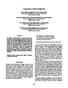
Figure 1: Relationships between di�erent object types. 3.1 Representing Spatial Relations by Intersection This step is described in more detail in �AEG95]. A brief overview of the representation approach is given below. The intersection-based representation of spatial relations is done in two basic steps: 1. Decomposition of the objects and the space into representative components. 2. Using the intersection of these components to represent the spatial relationships.
1. Object and Space Decomposition
If x is an object of interest then the result of the �rst step above is the representation Sofn x with a set of components x1 � x2 � � � � xn such that x = i=1 xi , and the complement of S x is also decomposed into components: x; = mj=n+1 xj . We use X to denote the space associated with the object x such that X = x � x; . An example of the decomposition for a line and an area objects is shown in �gure 1. In the �gure the components associated with the line x are X = x1 � x2 � x0 where x1 denote the set of two end points of the line. Similarly the components associated with the area y are Y = y1 � y2 � y0 . (The components x0 and y0 are the complements of objects x and y). The space in which the objects are embedded is considered to be dense and connected. Also the spaces associated with the objects considered are equal, i.e. X = Y in the above example (since both spaces are copies of the embedding space). Decomposition is carried out to re�ect important components in the application considered.
2. De�nition of Spatial Relationships
Using the above decomposition spatial relationships can be de�ned by the intersection of the components of the space associated with one object with those of the other. If R(x� y) is a relation of interest between object x and object y, and X and Y are the spaces associated with the objects respectively such that n is the number of components in X and m is the number of components in Y , then a spatial relation R(x� y) can be represented by one state of the following equation:
R(x� y) = X \ Y =
�n !
yj j=1 = (x1 \ y1 � x1 \ y2 � � � � � x1 \ ym � x2 \ y1 � � � � � xn \ ym ) i=1
xi
m ! �
\
xi \ yj can take the value � for an empty intersection or 6= � for a non-empty intersection. The set of intersections can be represented by an intersection matrix as follows2 : (
R x y
)=
x0
y0
y1
y2
x1 x2
.. .
2 This representation di�ers from that proposed in EF91] in that no constraint is imposed on the number or type of components used for representing the objects. In EF91] object representation is restricted to three components: interior, boundary and exterior.
� where i = 1� � � � n. This symbol indicates that the component yj intersects with every element in the set x0 and does not intersect with any element in the complement of x0 .
x0 y0 y0 x1
y3
x2
y3
x0 x1 x2 y1
y2
y1 x1 x2 x0
0 0 1
y2
y3
0 0 0 0 1 1 (a)
y1
y2
y0
y1
1 1 1
x1 x2 x0
0 0 1
y2
y3
y0
0 1 0 1 1 1 (b)
0 0 1
i �R] yj i � yj xi = yj xi � yj 0i j0 x = y xi \ yj = � x x
j
k
� z
1 1 1 1 0� 1
j = zk
y
1 1 1 1 0
j �R] zk 0 0 � zk y = z j k
y
j
y
0� 1 1 1 0� 1 0
0� 1 1 1 0� 1 0� 1
Rule0 1 Propagation of Non-Empty Intersections
Let z = fz1 � z2 � � � � � zn g be a subset of the set of components of space Z whose total number of components is n and n0 n� z 0 � Z. If xi, yj are components of spaces X and Y respectively, the following is a governing rule of interaction for the three spaces X, Y and Z. 0
Figure 2: A possible decomposition of the space to distinguish the relationships between objects x and y in (a) and (b). 0 is used in the matrix to denote empty intersection and 1 is used to denote non-empty intersection. y
The following subset relation can be concluded from table 1: (xi \ yj 6= �) ^ (yj � zk ) ! (xi \ zk 6= �) and (xi \ yj = �) ^ (yj zk ) ! (xi \ zk = �). This rule can be generalized as follows,
j \ zk = �
y
0 0 0� 1 0� 1 0� 1
Table 1: Transitivity table of subset relations between single components. The compositions are expressed in terms of intersection of the components xi and zk . Distinguishing qualitatively di�erent spatial relationships is dependent on the strategy used in the decomposition of the objects and their related spaces. The example in �gure 2 demonstrates a possible decomposition of an object to distinguish qualitatively di�erent relationships. The method is �exible and allows the use of virtual components (without physical boundaries) to represent the application considered. 3.2 Spatial Reasoning rules Composition of spatial relations using an intersection representation is based on the transitive property of the subset relations. Let xi be one component of the set X , yj a component of the set Y and zk a component of the set Z . Table 1 demonstrate the composition of subset relations where the resultant relation xi �R] zk is interpreted as the intersection between the two components. Here (1) represents a non-empty intersection, (0) an empty intersection and (0� 1) represents the inde�nite case. The �rst four rows in table 1 are the cases where the two components xi and yj have a non-empty intersection. Compiling these �rst four cases, it can be seen that the composition of relations can result in a de�nite intersection in only two cases, namely, when yj � zk and yj = zk . In the rest of this paper the following subset notation is used. If x0 is a set of components (set of point-sets) fx1 � � � � � xn g in a space X, and yj is a component in space Y, then v denotes the following subset relationship. yj v x00 denotes the subset relationship such that: 8xi 2 x (yj \ xi 6= �) ^ yj \ ( X ;x1 ; x2 � � � ; xn ) =
(xi \ yj 6= �) ^ (yj v z 0)
(xi \ z 0 6= �) xi \ z1 6= � _ � � � _ xi \ zn 6= � xi \ (z1 � z2 � � � � zn ) 6= � The constraint (xi \ z1 6= � � � � _ xi \ zn 6= �) can be expressed in the intersection matrix by a label, for example the label a in the following matrix indicates x1 \(z2 �z4 ) 6= �. ! � �
0
0
0
x1
z1 z2 z3 z4 ; a ; a
��� ;
zn ;
If two constraints overlap, for example, x1 \ z1 6= � _ x1 \ z2 6= � _ x1 \ z3 6= � (1) x1 \ z1 6= � _ x1 \ z3 6= � (2) only the stronger one, (2 in this case) has to be represented. Similarly, if the constraint x1 \ z1 6= � is derived, then both constraints 1 and 2 need not be represented. Rule 1 represents the propagation of non-empty intersections of components in space. A di�erent version of the rule for the propagation of empty intersections can be derived as follows,
Rule0 2 Propagation of Empty Intersections
Let z = fz1 � z2 � � � � � zn g be a subset of the set of components of space Z whose total number of components is n and n0 < n� z 0 � Z. If all the intersection relations of xi derived from rule 1 are given by xi \ z 0 6= � only, then it can be concluded that the intersection of the component xi with any set in the complement of z 0 is empty, i.e. xi \ ( Z ;z1 ; z2 � � �; zn ) = �. Remark: if n0 = n, i.e. xi may intersect with every component in Z, then no empty intersections can be propagated. Rule 2 is an implication of the assumption of dense, connected and equal spaces associated with the objects. The above two rules have to be applied for propagating the intersection of the components of both the objects involved, i.e. x and z . Rules 1 and 2 are the only two general rules necessary for propagating de�nite empty and non-empty intersections of components of spaces. The rules are expressed for spaces with random numbers of components and hence can be applied to di�erent space resolutions. In the rest of this paper examples are given to demonstrate the applicability of the reasoning rules for deriving deriving spatial relations between objects of di�erent types and random complexity. 0
0
x0
y0
z0
y0 z1
y1
y2
z2
x2
x1 x2
3.3 Reasoning with Objects of Di�erent Types The set of sound relations between regions and between lines and regions have been identi�ed �JB94]. An example of reasoning between regions and lines is shown in �gure 3. Relationships in the �gure are inside(x� y) and R15 (y� z ) from table 2. The matrices for the relations in the �gure are as follows. (
)=
y0
y1
1 0 0
x1 x2
y2
1 0 0
1 , I(y,z) = 1 1
z0
z1
1 1 1
y0 y1 y2
0 1 0
\y
6
� ^
v fz0 z2 g
y
x1 \ z1
intersections: From rule 1 we have, 2 2 = 2 From rule 2 we have,
=
!
x1 \
(
z0 � z2
\y
6
� ^
x2 \ z1
=
x1 x2 x3
x
\y
x
6
6
� ^ y
� ^ y
\y
6
z
\ y
v fz
� ^ y
!
x2 \
(
z0 � z2
)= 6
�
�
z g
!
x
\
z
�z
z g
!
x
\
z
�z
v fz
z g
!
x
\
z
�z
z
^ y
v fx g !
\x
�
^ z
6
�
�z 6
6
�
�
z
\x
\ x
6
�
�
� z
z
z
\y
z
\y
\y
6
6
�
6
�
^ y
v fx g !
z
\x
6
�
�
^ y
v fx g !
z
\x
6
�
x
�x
� x
^ y
v fx
x
x g !
z
\
6
�
6
�
� z
z
\y
z
\y
6
�
^ y
v fx g !
z
\x
6
�
z
\y
6
�
^ y
v fx g !
z
\x
6
�
x
�x
� x
6
�
^ y
v fx
x
x1 x2
1 0 0
x0
z2
1 1 1 1
y1
1 0 0 1 (a)
y2
1 0 0 1
y3
z3
z0
1 0 0 1
y0 y1 y2 y3
z0 x0 1 x1 a x2 b
�
� z
6
z1
1 1 1
1 1 1 1
z1
0 0 0 1 (b)
z2
0 0 0 1
z3
0 0 0 1
No empty intersections can be propagated in this case. Re ning the above constraints, we have the following intersection matrix.
z
v fz
z0
x0
Figure 5: Relationships between two concave regions, between x and y in (a) and y and z in (b).
�
intersections: From rule 1 we have, 0 0 = 0 0 2 0 ( 0 2) = 0 1 = 1 0 1 2 0 ( 0 1 2) = 0 2 = 2 0 2 0 ( 0 2) = No empty intersections can be propagated in this case. 1 intersections: From rule 1 we have, 1 1 = 1 0 1 0= From rule 2 we have, 1 1= 1 2= 2 intersections: From rule 1 we have, 2 0= 2 0 = 0 0 2 1 = 1 0 2 0= 2 2 = 2 0 1 2 2 ( 0 1 2) = No empty intersections can be propagated in this case. 0 intersections: From rule 1 we have, 0 0 = 0 0 0 0= = 0 1 1 0 0 0= = ( 0 2 2 0 1 2 0 0 1 2) = \y
1 1 0
y2
x3
y0 x0
� x0
x
z2
z1
�
v fz0 z2 g
y
x2
1 0 0
y3
� x2
x
x1
z1
z0
1 1 1
6
1 1 1
y1 x2
z2
)=
z0
x0
y0
x0
� x1
x
1 0 0
x1
The reasoning rules are used to propagate the intersections between the components of objects x and z as follows. intersections: From rule 1 we have, 1 2 = 2 From rule 2 we have,
z2
1 0 0
Figure 4: Possible relations resulting from the composition in �gure 3.
Figure 3: Relationships between di�erent object types.
x0
z1
1 1 1
x0
y2 z1
I x y
z0
y1
x1
x g !
z
\
z1 z2
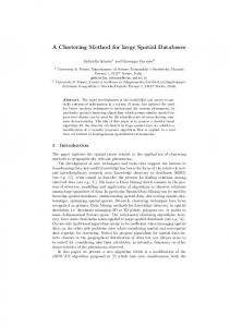
1 1 0 a 0 b The matrix represents the possible relations in �gure 4 which correspond to relations R1 , R18 and R19 in table 2. The full composition table for reasoning over lines and regions is given in table 2. 3.4 Reasoning with Complex Objects Cohn et al �CRCB93] proposed de�nitions of spatial relationships between concave shaped objects (representing solid bodies). They distinguished between the relationships topologically inside (where one body is physically inside the interior of another) and geometrically inside (where one body lies inside the convex hull of another). They used a convex hull function for the de�nition of the latter relationship. The convex hull of a region is outlined by the dotted line as in �gure 5. In �CRCB93] they presented the composition table for these concave regions. In this example we demonstrate the applicability of the reasoning rules proposed here by the systematic derivation of composition of spatial relationships between concave regions which comprise the entries of the presented composition table. Consider the example in �gure 5 where the relationships between three solid concave shaped bodies x, y and z are shown. Using a similar method as that of the previous example, the propagated constraints are as follows, x1 \ z0 6
=
�
^ x1 \ z1
=
� ^ x1 \ z2
=
�^
z2
1 1 1
Figure 6: Resulting relations from the composition in �gure 5. The symbols are used to identify the relations in (Cohn et al �93]). =
x2 \ z0 6
x1 \ z3 �
^ x2 \ z1
=
x2 \ z3
= 3 = 3=
z1 \ x3 6
=
� ^ x2 \ z2
=
=
� ^ x1 \ z4
=
�
� ^
= 3 0 = 0 0 = () 0 = () 0 = () 0 =
� ^ x2 \ z4 \z
6
x
\z
6
� _ z1 \ x
x
�
6
� �
�
a
z2 \ x
6
� _ z2 \ x
6
�
b
z3 \ x
6
� _ z3 \ x
6
�
c
The constraints matrix is therefore as follows, (
I x z
)=
z1
z2
z3
x3
a
b
c
x0
a
b
c
x1 x2
0 0
0 0
0 0
z0
1 1 1 1
The resulting matrix represents the four possible relations in �gure 6. Only three of the relations in �gure 6 (the �rst two and the last relation) are presented in the work of �CRCB93]. 4 Comparison with Related Work Earlier work on spatial reasoning has been carried out on simple objects whose dimension is equal to the dimension of the space in which they are embedded. Two spatial reasoning tasks can be identi�ed: Deriving composition tables: Composition tables for simple regions in 2D space were derived by Egenhofer �Ege94] using transitivity of the subset relations and by Cohn et al �CRCB93] using a theorem proving approach. In the latter work the composition table for concave solid objects has also been presented. Consistency Checking: Spatial reasoning has been applied to check the consistency of a scene of simple regions in �SP92, ES92]. The reasoning method used is based on exploiting composition tables to propagate constraints in network. 5 Conclusions In this paper a general method for the reasoning over topological relations between objects of random complexity in any embedding space is presented. The following conclusions can be drawn. The reasoning process is simple and is based only on two reasoning rules: one for deriving non-empty intersections of object components and another for deriving empty intersections. The two rules are applicable to objects of any complexity in any space dimension.
The reasoning method is capable of deriving composition tables for any con�gurations and space dimension when all the sound relations in the domain are known. A new composition table is presented as a result of the implementation of this method. This work is part of an ongoing research program for the application of deductive object-oriented databases for geographic data handling �AEG94, APW+ 94]. References �AEG94]
Alia I. Abdelmoty and B.A. El-Geresy. An Intersection-based Formalism for Representing Orientation Relations in a Geographic Database. In 2nd ACM Workshop On Advances In Geographic Information Systems. ACM press, December 1994. �AEG95] Alia I. Abdelmoty and B.A El-Geresy. A General Approach to the Representation of Spatial Relationships. Technical Report CS-95-6, Department of Computer Studies, University of Glamorgan, Wales, 1995. �APW+ 94] Alia I. Abdelmoty, Norman W. Paton, M. Howard Williams, Alvaro A.A. Fernandes, Maria L. Barja, and Andrew Dinn. Geographic Data Handling in an Deductive Object-Oriented Databas e. In D. Karagiannis, editor, Proc. 5th International Conference on Database and Expert Systems Applications (DEXA), pages 445{454. Springer Verlag, Sep 1994. �CRCB93] A.G. Cohn, D.A. Randell, Z. Cui, and B. Bennet. QualitativeSpatial Reasoning and Representation. In P. Carrete and M.G. Singh, editors, Qualitative Reasoning and Decision Technologies, 1993. �EF91] M.J. Egenhofer and R.D. Franzosa. PointSet Topological Spatial Relations. Int. J. Geographic Information Systems, 5(2):161{174, 1991. �Ege94] M.J. Egenhofer. Deriving the composition of Binary Topological Relations. Journal of Visual Languages and Computing, 5:133{149, 1994. �ES92] M.J. Egenhofer and J. Sharma. Topological consistency. In P. Bresnahan, E. Corwin, and D. Cowen, editors, Proceedings of the 5th International Symposium on Spatial Data H andling, volume 2, pages 335{343, Charleston, 1992. IGU Commission of GIS. �FNF91] K.D. Forbus, P. Nielsen, and B. Faltings. Qualitative Spatial Reasoning: the CLOCK Project . Arti�cial Intelligence, 51:417{471, 1991. �Gue89] Guesgen, H.W. Spatial reasoning based on allen's temporal logic. Technical Report TR-89-049, International Computer Science Institute, Berkeley, California, 1989. �JB94] T.Y. Jen and P. Boursier. A Model for Handling Topological Relationships in a 2D Environment. In Proceedings of the 6th international Symposium on Spatial Data Handling, volume 1, pages 73{89, 1994. �MJ90] A. Mukerjee and G. Joe. A Qualitative Model for Space. In Proceeding of the 8th National Conference on Arti�cial Intellige nce, AAAI, 1990, pages 721{ 727, 1990. �RCC92] D.A. Randell, A.G. Cohn, and Z. Cui. Computing Transitivity Tables: A Challenge for Automated Theorem Provers. In CADE, Lecture Notes In Computer Science, 1992. �SP92] T.R. Smith and K.K. Park. Algebraic Approach to Spatial Reasoning. International Journal of Geographic Information Systems, 6(3):177{192, 1992.
disjoint(x y) x
y
meet(x y) x
y
inside(x y) y x
coverdBy(x y) x
contain(x y)
cover(x y) y
y
y x
x
overlap(x y) x
R1 (y z)
all
all
1
1
all
all
all
R2 (y z)
1 2 4 16 17 18 19
1 2 3 4 5 6 7 8 9 10 14 15 16 17 18 19
1
1 2
9 10 11 12 13 14 17
2 3 4 5 6 7 8 9 10 11 12 13 14 15 16 17
all
R3 (y z)
1 18 19
1 2 3 4 5 6 7 8 15 16 18 19
1
1 2 3
11 12 13
3 5 6 7 8 9 10 11 12 13 14 15
all
R4 (y z)
1 2 4 16 17 18 19
1 2 3 4 5 6 7 9 14 15 16 17 18 19
1
1 2 4 19
9 10 11 12 13 14 17
4 5 6 7 8 9 10 11 12 13 14 15 16 17
all
R5 (y z)
1 18 19
1 2 3 4 5 6 7 15 16 18 19
1
1 2 3 4 5 19
11 12 13
5 6 7 8 9 10 11 12 13 14 15
all
R6 (y z)
1
1 2 3 4 5 6 19
1
1 2 3 4 5 6 19
11
6 7 8 9 10 11 12
all
R7 (y z)
1
1 2 3 4 5 19
1 18 19
1 2 3 4 5 6 7 15 16 18 19
11
7 8 9 10 11 12
all
R8 (y z)
1
1 2 3
1 18 19
1 2 3 4 5 6 7 8 15 16 18 19
11
8 10 11
all
R9 (y z)
1
1 2 4 19
1 2 4 16 17 18 19
4 5 6 7 8 9 10 11 12 13 14 15 16 17
11
9 10 11 12
all
R10 (y z)
1
1 2
1 2 4 16 17 18 19
1 2 3 4 5 6 7 8 9 10 14 15 16 17 18 19
11
10 11
all
R11 (y z)
1
1
all
all
11
11
all
R12 (y z)
1
1 19
1 2 3 4 5 13 14 15 16 17 18 19
1 2 3 4 5 6 7 9 12 13 14 15 16 17 18 19
11
11 12
all
R13 (y z)
1 18 19
1 18 19
1 2 3 4 5 13 14 15 16 17 18 19
1 2 3 4 5 13 14 15 16 17 18 19
11 12 13
11 12 13
all
R14 (y z)
1 18 19
1 2 4 16 18 19
1 2 4 16 17 18 19
1 2 3 4 5 14 15 16 17 18 19
11 12 13
9 10 11 12 13 14
all
R15 (y z)
1 18 19
1 2 3 4 5 15 16 18 19
1 18 19
1 2 3 4 5 15 16 18 19
11 12 13
7 8 9 10 11 12 13 14 15
all
R16 (y z)
1 2 4 16 17 18 19
1 2 3 4 5 14 15 16 17 18 19
1 18 19
1 2 4 16 18 19
9 10 11 12 13 14 17
7 8 9 10 11 12 13 14 15 16 17
all
R17 (y z)
1 2 4 16 17 18 19
1 2 4 16 17 18 19
1 2 4 16 17 18 19
1 2 4 16 17 18 19
9 10 11 12 13 14 17
9 10 11 12 13 14 17
all
R18 (y z)
1 2 3 4 5 13 14 15 16 17 18 19
1 2 3 4 5 13 14 15 16 17 18 19
1 18 19
1 18 19
7 8 9 10 11 12 13 14 15 16 17 18
7 8 9 10 11 12 13 14 15 16 17 18
all
R19 (y z)
1 2 3 4 5 13 14 15 16 17 18 19
1 2 3 4 5 6 7 9 12 13 14 15 16 17 18 19
1
1 19
7 8 9 10 11 12 13 14 15 16 17 18
4 5 6 7 8 9 10 11 12 13 14 15 16 17 18 19
all
y
Table 2: The composition table between two regions and a region and a line. The numbers in the table correspond to relations R1 to R19 between a region and a line.