A Clustering Method for large Spatial Databases Gabriella Schoier1 and Giuseppe Borruso2 1
2
Universit´ a di Trieste, Dipartimento di Scienze Economiche e Statistiche, Piazzale Europa 1, 34127 Trieste, Italia,
[email protected] Universit´ a di Trieste, Centro d’ecellenza in Telegeomatica-GeoNetLab,Dipartimento di Scienze Geografiche e Storiche,Piazzale Europa 1, 34127 Trieste, Italia
Abstract. The rapid developments in the availability and access to spatially referenced information in a variety of areas, has induced the need for better analysis techniques to understand the various phenomena. In particular spatial clustering algorithms which groups similar spatial objects into classes can be used for the identification of areas sharing common characteristics. The aim of this paper is to present a density-based algorithm for the discover of clusters in large spatial data set which is a modification of a recently proposed algorithm.This is applied to a real data set related to homogeneous agricultural environments.
1
Introduction
The paper explores the spatial issues related to the application of clustering methods to geographically relevant phenomena. The development of new techniques and tools that support the human in transforming data into useful knowledge has been the focus of the relatively new and interdisciplinary research area: knowledge discovery in databases (KDD) (see e.g. [1]), term coined to describe the process for finding relations among observed data (see e.g. [1]). His heart is Data Mining which consists in the process of selection, modelling and application of algorithms to discover relations among large quantities of data. In particular Spatial Data Mining can be used for browsing spatial databases, understanding spatial data, discovering spatial relationships, optimizing spatial queries. Recently, clustering techniques have been recognized as primary Data Mining methods for knowledge discovery in spatial databases, i.e. databases managing 2D or 3D points, polygons etc. or points in some d-dimensional feature space. The well-known clustering algorithms, however, have some drawbacks when applied to large spatial databases (see e.g. [4]). On one side traditional algorithms seems to be inefficient when managing spatial data; on the other side problems arise when considering spatial and non-spatial data together for clustering. Suited for purpose algorithms for spatial data detects clusters in the geographical distribution of data but not always seem to be suited for considering also their attributes, as intensity, frequency or other characteristics of the phenomena observed. In this paper we present a new algorithm which is a modification of the DBSCAN algorithm proposed in [2] which take into consideration both the
2
spatial aspect and the non spatial variables relevant for the phenomenon that has to be analyzed. Homogeneous agricultural environments are used as a case study for our analysis.
2
The proposed Spatial Clustering Algorithm
Spatial clustering is a method of spatial data analysis, which has been used widely in fields like medicine, ecology, urban studies etc.. Its aim to create groups of units so that there is a high degree of similarity inside the group but a high degree of dissimilarity among elements of different groups. There are different types of clustering algorithms: the partitioning methods,the hierarchical methods,the density-based methods and the grid methods [2]. Many factors are involved in the choice of the algorithm in the application to large databases,the tradeoff between quality and speed, the capacity of discovering clusters of arbitrary shape and the characteristics of the data. In this paper we will consider clustering methods based on the notion of density. These regard clusters as dense regions of units which are separated by regions of low density (representing noise), they may be used to discover clusters of arbitrary shape.Among these the DBSCAN [2] judge the density around the neighborhood on an unit to be sufficiently dense if the number of points within a distance EpsCoord of an unit is greater than MinPts , in this case the unit is a core point otherwise is a border point [2]. This algorithm has been generalized in [7] by considering the GDBSCAN that can cluster points units such as spatially extended units. Our proposed generalization ”the Modified Density-Based Spatial Clustering of Applications with Noise” M DBSCAN considers an approach density based that take into account at the same time the spatial variables and the non spatial variables. It has a similar structure of the DBSCAN but introduce a notion of proximity not only for spatial characteristics but also for non spatial characteristics. The key idea is that the cardinality of the neighborhood of an unit is given not only by counting the number of units that have distance from it less than the radius EpsCoord but by the points that have distance less than EpsCoord and that are ”sufficiently” similar as regards non spatial attributes. In order to have a sufficient homogeneity for the non spatial attributes another radius Eps that represent the threshold for the distances calculated on the bases of the non spatial variables is evaluated. In so doing we want to find clusters of elements which are spatially close to each other and homogeneous as regards other observed variables.The elements of such a clusters may be interpreted as elements similars as regards some variables and that belong to the same spatial area. In the following we present the main steps of the algorithm
3
Algorithm 1 (MDBSCAN) Step 1. Insert the values of the parameters: SetOfPoints representing the matrix with the values of the non spatial variables,Coordinates representing the spatial variables ,Eps the limiting distance value for the non spatial variables ,EpsCoord the limiting distance value for the spatial variables,MinPts the minimum number of points to consider a point as a core point. Step 2.Chose an arbitrary point i in the database if i is a core point built the cluster by choosing all the points which are density-reachable from i else if it is a border point the algorithm pass to the point i+1 Step 3.Classify the points which are not density-reachable as noise The value of the parameter MinPts is fixed as in [2]). In order to determine the parameter EpsCoord, regarding the spatial variables, and the parameter Eps, regarding the non spatial variables that are considered important for explaning the phenomenon of interest, we consider the algorithms SorteKdist and respectively SorteKdist2 . The former evaluates, for every point of the database represented by the matrix Coordinates, the distances from the nearest k-points (belonging to the same database),orders them in decreasing way and gives a graphical representation of these distances. The latter is similar, it evaluates, for every point of the database represented by the matrix SetOfPoints, the distances from the nearest k-points (belonging to the same database) and gives the mean value. As regards the algorithm SorteKdist uses the spatial variables; it is implemented following [2]; it evaluate for every unit of the input database the distances from the k nearest points (for the choice of k see [7]) ,it orders the distances gives a graphical representation. The algorithm SorteKdist2 uses the non spatial variables, it evaluate for every unit of the input database the distances from the k nearest points and gives the mean values.
3
An application on a real dataset
In order to test the algorithm and the chosen procedure, we have examined a spatial database containing municipalities in the Friuli Venezia Giulia Region in Northeastern Italy for the year 1990. The aim is relating the spatial position of municipalities with a particular set of indices of performance of the agricultural sector in order to obtain a zoning system of municipalities in terms of both location and structural and economical characteristics. Such zoning should therefore allow a classification of agricultural zones according to their characteristics of production and structure to supply public authorities with a tool for examining performances in different parts of the Region ([6]). Different indicators have been used to classify the different municipalities according to their characteristics. The method involved examining the productive structure of the agricultural sector referred to the smallest area. Municipalities represent the smaller spatial unit for which data are available. Both static and dynamic indices have been used in order to evaluate the weight
4
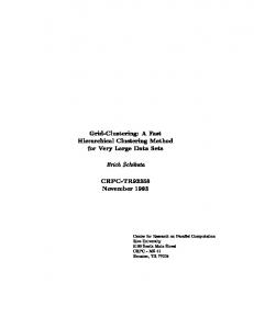
of agricultural in the demographic environment; the diffusion of agricultural entrepreneurship; the presence and diffusion of small-size forms (pulverization); the diffusion of entrepreneur as main actor in the firm. Agricultural land use has also been considered as well as density of bovine stock-farm. Moreover the coordinates have also been used as variables for the spatial clustering analysis performed. In this stage we considered the coordinates of municipalities’ that is the centroids. The database obtained contained therefore the following data referred to municipalities in the Region. Only lowland municipalities were considered so we examined 111 municipalities over a total of 219. The M DBSCAN algorithm implemented involved choosing different thresholds for the coordinates and for the other indices. As regards the spatial variables the algorithm SorteKdist has been implemented the result is represented in Fig. 1
k−dist
2000
4000
6000
8000
10000
Sorted k−dist graph
0
20
40
60
80
100
Points
Fig. 1. Determination of the parameter EpsCoord Looking at the graph we have chosen EpsCoord = 7741 that is the first point in the first valley [2]. As regards the non spatial variables the algorithm SorteKdist2 has been implemented the result is Eps = 1.71 At this point we have applied the M DBSCAN . the variables used are: Sj ( agricultural land use), Rj (weight of agriculture in the economical system), zj (agricultural entrepreneurship), dj (agricultural firms’ pulverization (number of firms)); d1j (agricultural firms’ pulverization (surface of firms)), tj (diffusion of entrepreneur as main actor), aj (agricultural surface used for sown), doj (agricultural surface used for permanent cultivations), pj (density of bovine stock-farm), gj (dynamic of firms lead by working firm); XCOORD (X coordinate (Eastings) in UTM 33 ED50 reference system), Y COORD (Y coordinate (Northings) in UTM 33 ED50 reference system.) The distance used for running our algorithm is the euclidean one.
5
Interesting results arise after performing the cluster analysis on the dataset. Fig. 2 shows the results of the analysis.
Fig. 2. Spatial clusters of municipalities of the region F.V.G.
The algorithm has detected four clusters and classified 24 municipalities as ’noise’, therefore not belonging to none of the clusters detected. If compared to other traditional, non-spatial techniques applied in the past, spatial clustering allow a more homogenous zoning of municipalities, with the most of them belonging to a cluster contiguous and close to each other. From this point of view therefore the algorithm seems to operate proficiently in order to obtain a spatial zoning of the municipalities considered. As threshold plays a key role in determining if a municipality belongs or not to a cluster, different threshold could be tested in order to allocate all the municipalities in a cluster. At this stage it is anyway interesting that most of the municipalities are allocated and continuous. When moving to examining the different non-spatial indices we can observe interesting dynamics taking place over the municipalities in the lowland area. The exam of Fig. 3 can help in examining the characteristics of the different clusters in terms of the indices used.
6
Fig. 3. Average values of the indices. The graph was built calculating mean values of each index for each cluster. A selection of indices has been done as pivot variable to characterize the clusters. In particular, Sj , zj dj , tj aj have been analyzed. Only the first three ones however present some diversities in their figures, while the other ones present values very close to each other. As regarding a general analysis on the composition of the clusters Cluster 2 seems to be the more proficient one in terms of agricultural performance. This can be said after examining the general performance over the entire set of indicators. It present higher values than the other ones in the most of the indices observed, with particular reference to the agricultural entrepreneurship, weight of agriculture in the economical system, agricultural firms’ pulverization (surface of firms) and dynamic of firms lead by capitalistic firm. Cluster 3 follows, characterized mainly by high values of agricultural land use and low values of agricultural surface used for permanent cultivations. Cluster 3 and Cluster 4 follow in the lower end of the class, displaying quite close values in he most of the indices, apart for the agricultural entrepreneurship, where Cluster 4 present lower values. As a general impression on the results obtained from the analysis of indices we can however notice that different in mean values between different clusters are not so high: that can mean that the general situation of agriculture portrayed in the Region is quite a homogeneous one and differences can be attributed to different shape of small areas used (municipalities) as well as to micro-economical characteristics of firms.
4
Conclusions
The spatial clustering analysis allowed in any case to group together municipalities according to the values offered by the indices and therefore also small differences in values allow to discriminate between clusters. In this paper we present a new algorithm which is a modification of the DBSCAN algorithm proposed in [2] which take into consideration both the
7
spatial aspect and the non spatial variables relevant for the phenomena that has to be analyzed. Homogeneous agricultural environments are used as a case study for our analysis. Further research is however necessary with particular reference to the spatial component of the data. At this stage we considered centroids of municipalities as identifiers of geographical location. In geographical terms, municipalities are represented by means of irregularly-shaped polygons, with very different characteristics of surface, perimeter and attributes that can be related to them. There is the risk that, given a certain threshold, only small-area municipalities clusters while larger ones tend to be left out or considered as belonging to a different cluster. The topics to tackle in the future involve therefore considering polygons for the cluster analysis instead of their centroids’ coordinates.
References [1] Bailey, T. C., Gatrell, A. C.:Interactive spatial data analysis. Addison Wesley Longman Edinburgh, UK.(1995) [2] Ester, M., Kriegel, H.,P.,Sander, J.,Xiaowei, X.: A Density-Based Algorithm for Discovering Clusters in Large Spatial Databases with Noise.Proceeding of the 2nd International Confererence on Knowledge Discovery and Data Mining.(1996) 94–99 [3] Fayyad, U., Piatesky -Shapiro, G.,Smyth, P., From Data Mining to Knowledge Discovery in Databases. (1996) http : //www.kdnuggets.com/gpspubs/aimag−kdd− overview − 1996 − f ayyad.pdf [4] Han, J., Kamber, M., Tung, A.K.H.: Spatial Clutering Methods in Data Mining: A Survey. (2001) f tp : //f tp.f as.sf u.ca/pub/cs/han/pdf /gkdbk01.pdf. [5] Koperski K., Han J.,Adhikary J.: Mining Knowledge in Geographical Data.(1998) f tp : //f tp.f as.sf u.ca/pubcs/han/pdf /geos urvey98.pdf. [6] Prestamburgo M.:La classificazionedegli ambiti agricoli: una proposta metodologica. (1981) [7] Sander, J.,Ester, M., Kriegel, H.,P.,Xiaowei, X.: Density-Based Clustering in Spatial Databases: The Algorithm GDBSCAN and its applications.(1999) http : //www.dbs.inf ormatik.uni − muenchen.de/P ublikationen/