Home
Add Document
Sign In
Create An Account
A General Probabilistic Forecasting Framework for ... - DTU Orbit
Recommend Documents
Environmental exposure assessment framework for ... - DTU Orbit
Department of Environmental Engineering, Technical. University of .... 2013) or as waste electrical and electronic equipment (Directive 2012/19/EU). As.
ARTS: A System-Level Framework for Modeling MPSoC ... - DTU Orbit
Jan 15, 2010 - System-level models for design space exploration of em- bedded systems targeted .... Case Study Platform Architectures. cated for the whole ...
A baseline probabilistic drought forecasting framework using ...
Jul 4, 2014 - standardized soil moisture index: application to the 2012 United. States drought ... Global Integrated Drought Monitoring and Prediction Sys-.
Model-based Computer-aided Framework for Design of ... - DTU Orbit
Aug 31, 2009 - First of all, I would like to thank my supervisors Professor Rafiqul Gani and. Associate ...... Figure 1.1: Fixed process versus PAT based process.
s Single ... - DTU Orbit
Jan 22, 2010 - second-order pumpingâare evaluated numerically for 160-Gb/s ... In this letter, we focus on 160-Gb/s single-channel systems and the use of ...
YSZ Electrode - DTU Orbit
gated to the hydrogen electrode/electrolyte interface during electrolysis testing. ..... Si glass found at the interface of a long-term tested Ni-YSZ (anode)/.
BMC Bioinformatics - DTU Orbit
Aug 28, 2007 - The MaxAlign web-server is freely available online at http://www.cbs.dtu.dk/services/ ..... rent algorithms and implemented all the final software.
Conference paper - DTU Orbit
T20 according to ISO 3382-2 [11]. Max. in each 1/1 octave band. 125Hz: Max. + 20% accepted. Requirements implemented in. BC in 2008 and unchanged in.
Molecular biology - DTU Orbit
1Institute of Molecular Biology, National Academy of Sciences of the Republic of Armenia, 7 Hasratyan Str., 375044 Yerevan,. Armenia, e-mail:
[email protected]
...
eDNA - DTU Orbit
... our self-organisation and self-healing algorithms and the results obtained from this looks .... Figure 1 shows a sketch of the complete system. It also shows the ...
18 point - DTU Orbit
Krzysztof Iwaszczuk,1 Andrew C. Strikwerda,2 Kebin Fan,3 Xin Zhang,3. Richard D. Averitt,2 and Peter Uhd Jepsen1,*. 1DTU FotonikâDepartment of Photonics ...
Environmental Science - DTU Orbit
Feb 26, 2014 - Dorothea Gilbertc and Matthew MacLeoda. Passive equilibrium ...... 8 S. Endo, T. N. Brown and K.-U. Goss, Environ. Sci. Technol.,. 2013, 47 ...
Postprint - DTU Orbit
The thesis introduces the Double Travelling Salesman Problem with Mul- tiple Stacks ... og afprøves forskellige matematiske formuleringer i den anden artikel.
EDISON Project - DTU Orbit
tributed Energy Resources, Distributed Production, Demand. Response, Vehicle ... the EVs and renewable energy resources into virtual power plants (VPP) [3] ...
Paper title - DTU Orbit
New reference object for metrological performance testing of industrial ... The CT ball plate features a regular 5 x 5 array of ruby spheres with a nominal diameter ...
Euronoise 2006 - DTU Orbit
Two sources were taken into account: Street Traffic Sound (STS), and ... STS, NA is defined as 40 to 45 dBA, SA as 55 to 60 dBA, MA as 65 dBA, HA as 75 dBA ...
FA7 - DTU Orbit
W.W. Zhou and. M. Blanke. Servolaboratory, build. 326. S6ren T. Lyngs~ A'S ..... 400.0. 150.0. 200.0. 250.0. 300.0. 350.0. NUMBER OF SAMPLES (-05 SEC) ?-
NN ... - DTU Orbit
the TIMIT 39 phoneme task. ... Downloaded on March 09,2010 at 06:34:17 EST from IEEE Xplore. .... nizing five broad phoneme classes in the TIMIT database:.
Postprint - DTU Orbit
Haftka and Walsh[1], Nagendra et al. [2], Le Riche and Haftka. [3], Gürdal et al. ..... [3] Le Riche R, Haftka R. ”Optimization of laminate stacking sequence for ...
ultimate strength - DTU Orbit
Aug 21, 2009 - Concern for the ductile behaviour of ships and offshore structures and ... Ultimate Strength; Ultimate Limit States; Ultimate Limit State Design; Buckling ...... Mode IV: Local buckling of stiffener web (after buckling collapse of ...
Integrating Wind - DTU Orbit
ator as this may in some circumstances be the best ..... FIGURE [5]: PSD's of measured and simulated wind power producti
41 Turbine ... - DTU Orbit
to a single rotor case, the NORDTANK 500/41 rotor with LM19.1 blades. The transitional computations show improved agreement with measurements for.
Nanoscale - DTU Orbit
consider two mechanisms of electron emission from the nanoparticles â surface and volume ones â ... electronics31 â i.e. in all areas of science and technology where ... fDTU Fotonik, Technical University of Denmark, Шrsteds Plads 343, DK-2800
carisma 2012 - DTU Orbit
Sep 5, 2012 - James E. McGrath - Virginia Tech. (US) .... Chalmers University of Technology. Sweden. 38. 11:30 ...... aCellEra (
[email protected]
),. Summary.
A General Probabilistic Forecasting Framework for ... - DTU Orbit
Download PDF
1 downloads
0 Views
1MB Size
Report
Comment
Mar 7, 2012 -
AutoRegressive Conditional Heteroscedasticity
(GARCH) model, .... Volatility clustering and heteroscedasticity of the wind power time series.
Energies 2012, 5, 621-657; doi:10.3390/en5030621 OPEN ACCESS
energies ISSN 1996-1073 www.mdpi.com/journal/energies Article
A General Probabilistic Forecasting Framework for Offshore Wind Power Fluctuations Pierre-Julien Trombe ? , Pierre Pinson and Henrik Madsen DTU Informatics, Technical University of Denmark, Richard Petersens Plads 305, 2800 Kgs., Lyngby, Denmark; E-Mails:
[email protected]
(P.P.);
[email protected]
(H.M.) ?
Author to whom correspondence should be addressed; E-Mail:
[email protected]
; Tel.: +45-45253402.
Received: 9 January 2012; in revised form: 28 February 2012 / Accepted: 29 February 2012 / Published: 7 March 2012
Abstract: Accurate wind power forecasts highly contribute to the integration of wind power into power systems. The focus of the present study is on large-scale offshore wind farms and the complexity of generating accurate probabilistic forecasts of wind power fluctuations at time-scales of a few minutes. Such complexity is addressed from three perspectives: (i) the modeling of a nonlinear and non-stationary stochastic process; (ii) the practical implementation of the model we proposed; (iii) the gap between working on synthetic data and real world observations. At time-scales of a few minutes, offshore fluctuations are characterized by highly volatile dynamics which are difficult to capture and predict. Due to the lack of adequate on-site meteorological observations to relate these dynamics to meteorological phenomena, we propose a general model formulation based on a statistical approach and historical wind power measurements only. We introduce an advanced Markov Chain Monte Carlo (MCMC) estimation method to account for the different features observed in an empirical time series of wind power: autocorrelation, heteroscedasticity and regime-switching. The model we propose is an extension of Markov-Switching Autoregressive (MSAR) models with Generalized AutoRegressive Conditional Heteroscedastic (GARCH) errors in each regime to cope with the heteroscedasticity. Then, we analyze the predictive power of our model on a one-step ahead exercise of time series sampled over 10 min intervals. Its performances are compared to state-of-the-art models and highlight the interest of including a GARCH specification for density forecasts.
Energies 2012, 5
622
Keywords: wind energy; offshore; forecasting; Markov-Switching; GARCH; probabilistic forecasting; MCMC; Griddy-Gibbs
1. Introduction Climate change calls for the reduction of greenhouse gas emissions and thus a growing development of renewable energy sources. Benefiting from favorable governmental policies and large wind resources, countries in the north-west of Europe are rapidly increasing their wind power capacities. Historically, onshore installations have prevailed, but offshore wind energy is now growing significantly. In Denmark, the latest figures stated that wind power accounted for about 22% of the domestic electricity supply and, out of 3802 MW wind power capacity, 868 MW were installed offshore [1]. The current trend is towards the development of large-scale offshore projects capable of generating several hundreds of MW each. Indeed, sitting wind farms out at sea has substantial advantages of (i) more space available; (ii) a decrease of the frequency and duration of low wind speeds and (iii) an increased persistence for high wind speeds. Offshore wind farms are then expected to have higher capacity factors (i.e., the ratio of the actual power output over a given period of time to the maximum output if the wind farm had been operated at full capacity) [2]. However, in practice, integrating significant amounts of wind power into power systems remains a challenge and requires dedicated prediction tools for real-time monitoring, operation scheduling and energy trading. While most of these applications requires wind power forecasts in an hourly resolution, the recent deployment of large-scale offshore wind farms has increased the concern for forecasts with particular lead times of 5–10 min [3]. Indeed, power generation at large offshore wind farms turns out to be highly volatile, increasing the risk of imbalance in the power system, in the very short-term. This originates from the specific design of these wind farms which concentrate a large amount of wind power capacity within a relatively small area, increasing the impact of local meteorological phenomena (wind and rain fronts among others) on their short-term power production. For instance, measurements from the offshore site of Horns Rev reveal changes in the output power that may reach an amplitude of 60% the wind farm maximum capacity, within 15–20 min [4]. Such levels of fluctuations can rarely be observed onshore where similar capacities would be spread over a much wider area, smoothing out the effects of the weather instabilities [5]. Consequently, maintaining the short-term balance of the transmission system (i.e., matching the power supplied by the wind farm and the electricity demand) and the stability of the power system has become a critical issue and needs to be handled carefully to prevent potential damages (blackouts, etc.). At time-scales of a few minutes, wind power forecasts are preferably generated with statistical models, based on historical data only [6]. In the present paper, our aim is to introduce a case study of statistical modeling and forecasting of offshore wind power fluctuations and its related complexity from three perspectives:
Energies 2012, 5
623
• the modeling of a nonlinear and non-stationary stochastic process for which we propose a model that allows to capture up to three different time series effects: autocorrelation, heteroscedasticity and regime switching (the generic name of our model is MS-AR-GARCH), • the numerous issues linked to the practical implementation of such model as it requires an advanced estimation method based on a Markov Chain Monte Carlo (MCMC) algorithm, • the gap between applying such model to synthetic data and real world observations. This paper is organized as follows. Section 2 summarizes the latest achievements in wind power meteorology for very short-term applications and states the motivations for this study. Section 3 introduces the data and shows some of their major features. Then, in Section 4, specifications for the model we propose are discussed throughout a brief overview of the literature on Markov-Switching models which constitute a special class of regime switching models, and on GARCH models which are generalized forms of heteroscedastic models. Section 5 gives a detailed description of the estimation method based on a Markov Chain Monte Carlo algorithm and the reasons for such a choice. Applications to both synthetic and real data are presented and the accuracy and robustness of the estimation method are assessed. A forecast evaluation on real data is performed in Section 6 where the performances of our model are compared with current benchmark models for very short-term wind power fluctuations. Finally, Section 7 delivers concluding remarks. 2. Motivations Based on the State-of-the-Art First, with the planned deployment of large-scale offshore wind farms, there is an urging need to build up on the existing knowledge on these wind power fluctuations by characterizing the dynamics and identifying the factors which drive the wind power fluctuations in the very short-term. As a first step towards this understanding, Akhmatov et al. [7] reported that at a temporal resolution of 10 min, certain weather conditions at Horns Rev and in particular north-westerly winds very much favored large wind power fluctuations. Then, Sørensen et al. [8] proposed an aggregated model of individual wind turbines and showed its relative ability to simulate consistent wind power fluctuations at different time scales, from a few minutes up to 2 h ahead. Very recently, a spectral analysis of wind speed measurements at Horns Rev led to the identification of specific seasonal cycles as key features of wind variability [9]. Second, most of the state-of-the-art statistical methods gives focus to large prediction horizons, from 1 h to a couple of days, and show limited forecasting skills for very short-term horizons, within tens of a minute, at which large wind power fluctuations must be monitored [10]. This low level of predictability is due to the complex nonlinearities in the output power dynamics which cannot be captured by conventional models. Hence, there is a need for dedicated statistical methods capable of generating accurate forecasts for very short-term horizons. In that regard, our approach on forecasting is probabilistic and the respective performance of the models presented in this paper will be evaluated accordingly [11]. As a first attempt to deal with the low predictability of the output power of large-scale offshore wind farm, regime-switching approaches and more specifically Markov-Switching models have received a growing interest within the wind power community. Since their very first introduction in econometrics by [12], they have been commonly used in many disciplines such as speech recognition [13] or
Energies 2012, 5
624
computational biology [14], for instance. This class of models is prized for its ability to account for structural breaks or sudden changes in the process dynamics. In meteorology, Markov-Switching models are often used to estimate an unobservable climate state which ideally governs other climate variables such as wind speed or wind direction. For the specific case of large-scale offshore wind farms, the inferred states or regimes can be interpreted as changes of the wind farm behavior, in terms of power generation. Besides that, Markov Switching AutoRegressive (MSAR) models are shown to have better point forecast performances than AutoRegressive Moving Average (ARMA), Smooth Transition AutoRegressive (STAR) and Self-Exciting Threshold AutoRegressive (SETAR) [15]. Alternatively, a MSAR model is proposed in [16] with adaptive estimation of the parameters which allows parameter estimates to change over time to better account for the long-term variations of the wind characteristics. Density forecasts generated with that method are shown to be much sharper and have a better calibration than those generated with AR models. Nevertheless, one can argue that keeping the variance constant over time within each regime stands as a strong limitation for the forecasts sharpness when periods of different volatility levels alternate. This may mistakenly lead to over-determination of the optimal number of states when fitting the model to the data. One class of models capable of relaxing the constant variance assumption is the Generalized AutoRegressive Conditional Heteroscedasticity (GARCH) model, allowing the conditional variance in each regime to follow an ARMA process [17]. The GARCH class of models is appealing because it can cope with volatility clustering which is a clear issue when studying offshore wind power generation at high frequencies. Therefore, the present study proposes to extend MSAR models with a GARCH specification for the conditional variance dynamic in each regime (hence the resulting model name MS-AR-GARCH). This extension of the original MSAR model is expected to allow for a better identification of the volatility clustering effect and to a more parsimonious parametrization regarding the number of regimes. 3. Data from Large Offshore Wind Farms The data considered in the present study cover the time period from 16 February 2005 to 25 January 2006 and were recorded at Horns Rev I, the second largest offshore wind farm in operation in the world at that time. Horns Rev I is located 15 km away from the west coast of Jutland (Denmark) and consists of 80 turbines of 2 MW, for a nominal capacity of 160 MW. Original data were provided as individual time series of wind power measurements for each of the 80 turbines at one second time intervals. The original data are averaged in order to generate an aggregated time series of wind power fluctuations for the entire wind farm. A 10 min resolution is arbitrarily chosen within the range of values over which significant power fluctuations are observed [4]. Another reason to justify this choice is that grid operators monitor offshore wind farms at similar temporal resolutions [10]. The sampling procedure first consists in producing spatio-temporal averages over 10 min intervals for which a minimum of 75% of the data are of good quality. These averages are then normalized by the nominal capacity of the wind farm, following [18]. No attempt is made to fill in missing data points and many gaps remain present in the data. A 10 day episode of this time series is depicted on Figure 1. It can be noticed that the power generation is a double-bounded process, below and above. As a matter of fact, the power generation of a wind farm can neither be negative nor exceed its maximum capacity.
Energies 2012, 5
625
100 80 60 40 20 0
Normalized wind power [% of Pn]
Figure 1. Time series of normalized wind power generation at Horns Rev I over a 10 day episode in August 2005. The time series is sampled with a temporal resolution of 10 min.
04/08
05/08
06/08
07/08
08/08
09/08
10/08
11/08
12/08
13/08
Moreover, technical specificities and constraints of wind turbines make that wind power generation is not a linear function of the wind speed. The relationship between wind speed and power generation is described by the so-called power curve. This relationship is often estimated to convert wind speed forecasts into wind power forecasts. For a more detailed description of its use in practice, we refer to [19]. More generally, the power curve is considered a function of both the wind speed and the wind direction and must be estimated for every single wind farm. Nevertheless, wind speed and wind direction are not the only two factors that are believed to govern wind farm behavior. In the specific case of large offshore wind farms, it is also commonly assumed that complex local meteorological phenomena have a strong impact on the power generation. Ongoing research works on these phenomena are still in an early stage, and identifying them would require to combine both meteorological and statistical approaches which is not the purpose of this study. As for now, early assumptions based on empirical observations have described these phenomena as combinations of intense precipitations and wind gusts [20]. From Figure 1, one can see periods characterized by very different dynamics alternate with various frequencies and durations. This latter observation reveals the non-stationary behavior of this wind power time series, whatever the time scale one considers. This issue is further discussed in [9]. Non-stationarity is one of the reasons why most linear time series models show limited prediction skills. This feature is further illustrated on Figure 2 which plots the squared residuals of the best autoregressive model (of order 3), the associated autocorrelation function (ACF) and the partial ACF (PACF) for the wind power time series. The model was fitted to the whole time series, but to enhance visualization of the results, the squared residuals are only plotted for the period of time spanning from 1 August 2005 to 26 January 2006. First, a look at the squared residuals highlights the volatility clustering effect, meaning that large errors tend to be followed by large errors and similarly, small errors tend to be followed by small errors. It is a feature often observed for data sampled at a high frequency. Then, the ACF of the squared residuals indicates that the autocorrelation is significant up to very large lags which reveals the heteroscedastic behavior of the errors. Finally, the PACF allows one to evaluate the number of significant lags for the time series of squared residuals. It indicates that the conditional variance should be modeled as the weighted sum of approximately the last 20 squared errors. However, for the sake of parsimony, an
Energies 2012, 5
626
ARCH process of large order can well be substituted by a GARCH specification [17]. This well spread empirical approach offers the double advantage of drastically reducing the number of coefficients to be estimated while conserving the model adequacy. It also introduces a decreasing weight structure, from the most recent to the oldest past squared errors, for the computation of the conditional variance. Figure 2. Volatility clustering and heteroscedasticity of the wind power time series. (a) Squared residuals obtained after fitting an AR(3) model to the wind power time series; (b) Autocorrelation function of the squared residuals; (c) Partial autocorrelation function of the squared residuals. 5000
Squared residuals
4000 3000 2000 1000 0 Aug 05
Sept 05
Oct 05
Nov 05
Dec 05
Jan 06
Feb 06
(a)
Autocorrelation function
0.30 0.25 0.20 0.15 0.10 0.05 0.00 0
1
2
3
4
5
6
7
8
9
lags [in hours]
(b)
10
11
12
13
14
15
16
Energies 2012, 5
627 Figure 2. Cont.
Partial autocorrelation function
0.30 0.25 0.20 0.15 0.10 0.05 0.00 0
20
40
60
80
100
lags
(c) 4. Model Specifications 4.1. Wind Power Predictive Density As mentioned in the previous section, the time series of wind power is nonlinear and non-stationary. The smoothing effect outlined when considering a collection of wind turbines scattered over a wide area does not apply in the case of a single large-scale offshore wind farm. Furthermore, wind turbines do not generate electricity for wind speeds below the so called cut-in speed (∼4 m s−1 ) or above the the cut-off speed (∼25 m s−1 ). In addition, for wind speeds ranging from 15 m s−1 to 25 m s−1 , wind turbines operate at full capacity and produce a constant level of power. Consequently, the power generation drops to 0 or reaches its maximum in a significant number of occasions. From a statistical modeling perspective, it means that the process does meet its lower and upper bounds which generates mass points at the extremities of the wind power distribution. This prevents the use of a logistic transformation as adopted in [21] since the mass points would remain, even after transformation. In view of these limitations, truncated and censored normal distributions stand as appealing alternatives to the more classical Normal distribution. Recent developments that use the two former distributions applied to wind data include [22,23]. However, Markov-Switching models imply the computation of distribution mixtures. For the sake of the estimation method simplicity, we choose to consider neither the truncation nor the censoring of the Normal distribution since mixtures of these distributions would be too cumbersome to compute. For similar reasons, the Generalized Logit-Normal distribution as proposed in [24] was not considered. Finally, we focused on 2 symmetric distributions, namely the Student-t and Normal distributions. The Student-t distribution has the advantage of being more heavy-tailed than the Normal distribution, making the regimes more stable [25]. Its drawback is that it has one extra parameter (its degree of freedom) which is difficult to estimate [26]. The use of the Normal distribution, though
Energies 2012, 5
628
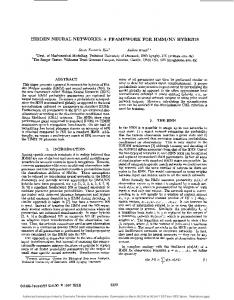
known as not optimal for wind power time series, is therefore considered as a natural starting point for testing the model in this study. We leave questions on more appropriate distributions for further research. 4.2. GARCH Models in Meteorology An overview of the time series analysis literature shows that GARCH models have been extensively used in econometrics and finance but remains rather unpopular in other fields. In meteorology, GARCH models are often employed in a single regime framework and applied to wind speed or air temperature time series for characterizing their volatility. Tol [27] first fitted an AR-GARCH model to daily wind speed measurements from Canada and illustrated the better in-sample performance of his heteroscedastic model over homoscedastic ones in presence of high volatility in the data. A bivariate GARCH model was then used in [28] to characterize the wind components (u,v) and their variability at a time scale of 1 min and relate them to local meteorological events in the Sydney harbor. Another meteorological application of GARCH models presented the usefulness of a ARMA-GARCH-in-mean model to estimate the persistence in the volatility of wind speed measurements at different heights [29]. In contrast to these latter studies whose primary focus is in-sample estimation, Taylor and Buizza [30,31] use AR-GARCH models to generate point and density forecasts for temperature and weather derivative pricing, respectively. In addition, the recent work by [32] also presents out-of-sample results. It extends the methodology developed in [30] and used several types of GARCH models to generate daily wind speed density forecasts and converts them into wind power forecasts. This work demonstrates the good ability of GARCH models for generating density forecasts when compared to atmospheric models for early look ahead horizons, from 1 up to 4 days. Another methodology is proposed by [21] in which an ARIMA-GARCH model is used to generate multi-step density forecasts of wind power, outperforming current benchmark models in the short-term, from 15 min up to 6–12 h. Interestingly, all these studies give empirical evidence of the strong potential of using the GARCH class of models for predicting weather related variables in the very short-term when these variables are highly volatile. 4.3. Existing Markov Switching Models with GARCH Errors Seminal references of combining Markov-Switching and AutoRegressive Conditional Heteroscedasticity (MS-ARCH) include [33] and [34]. In practice, capturing time-varying variance with a reasonable number of ARCH terms remains an issue. It often calls for a GARCH specification instead in order to reduce the number of coefficients to be estimated. The difficulty that arises when generalizing MS-ARCH to MS-GARCH relates to the historical path dependency of the conditional variance which is intractable, making that generalization almost computationally infeasible. Nevertheless, there exist a few approaches to avoid that problem. Regarding maximum likelihood methods, the idea consists in approximating the conditional variance as a sum of past conditional variance expectations as in [26]. This model was later extended by [25] yielding improved volatility forecasts. Alternatively, Haas et al. [35] suggested a new formulation for MS-GARCH models by disaggregating the overall variance process into separate processes in each regime. Another way of tackling the path dependency problem consists in using Monte Carlo Markov Chain (MCMC)
Energies 2012, 5
629
simulations to infer that path by sampling from the conditional distribution of the states of the Markov chain. This can be implemented by data augmentation as described in [36]. The strength of this approach is that it can be applied for the estimation of many variants of Markov-Switching models. Closer to our problem, Henneke et al. [37], Chen et al. [38], and Bauwens et al. [39] proposed three different MCMC algorithms for the Bayesian estimation of MS-ARMA-GARCH, MS-ARX-GARCH and MS-GARCH models, respectively. Some other difficulties arise when estimating MS-GARCH models. They may be caused by the structural specification of the model or else by the numerical tools used for parameter estimation. For instance, maximum likelihood estimation methods implemented with a numerical optimizer often encounter specific optimization problems due to starting values, inequality constraints or else local minima. Besides, the two formulations of the MS-GARCH model developed in [26] and [25] are based on an approximation for the recursive update of the conditional variance which leads to further estimation complexity. As for the MS-GARCH model in [35], it loses its initial appeal of being analytically tractable along with the inclusion of autoregressive terms in the conditional mean equation which does not match with our model specification to combine AR and GARCH effects with Markov-Switching. Along that last comment, it is important to emphasize that most of the studies involving likelihood estimation of MS-GARCH models have as a prime concern the capture of the heteroscedasticity present in the time series and were not designed to cope with data also featuring strong autocorrelation. In comparison, Bayesian inference offers an alternative framework which allows to overcome most of likelihood estimation problems: • the robustness of MCMC samplers to starting values can be evaluated by running several Markov chains with different starting values and tested for differences in their outputs, • inequality constraints can be handled through the definition of prior distributions (Gibbs sampler) or through a rejection step when the constraint is violated (Metropolis–Hastings sampler), • theoretically, local minima pitfalls are avoided by simulating the Markov chain over a sufficiently large number of iterations (law of large numbers), • misspecification of the number of states of the Markov chain can be assessed by a visual inspection of the parameter posterior distributions (check for multiple modes). Moreover, model parametrization limitations linked to the integration of autoregressive terms in the mean equation do not apply in Bayesian estimation and there is no fundamental implementation differences in estimating a MS-GARCH and a MS-ARMA-GARCH model. Of course, the present study would be very partial if the main bottlenecks in using MCMC simulations such as computational greediness or the tuning of the prior distributions were not mentioned. Therefore, we refer to Subsection 4.4 for a detailed description of the main implementation issues of MCMC samplers. In addition, studies on the respective advantages and drawbacks of maximum likelihood and Bayesian estimation methods are available in [40]. To conclude this discussion, let us say that our goal is not to contribute to the pros and cons debate of maximum likelihood against Bayesian estimation but rather to find the method that is the most suitable for our problem. In this light, our choice to estimate the MS-AR-GARCH model in a Bayesian fashion was motivated by the enhanced flexibility in combining AR and GARCH effects under the assumption of structural breaks in the process.
Energies 2012, 5
630
4.4. The Model Definition To model the stochastic behavior of a given time series of wind power {yt }, a MS(m)-AR(r)GARCH(p,q) model is proposed as follows: yt =
(S ) θ0 t
+
r X
(St )
θi
yt−i +
p ht εt
i=1 q (St )
ht = α0
+
X
(St ) 2 εt−i
αi
+
p X
(1)
(St )
βj
ht−j
(2)
j=1
i=1
where {ht } is the conditional variance at time t, {εt } is a sequence of independently distributed random variables following a Normal distribution N (0, 1) and S = (S1 , . . . , ST ) is a first order Markov chain with a discrete and finite number of states m and transition probability matrix P of elements: P r(St = j|St−1 = i) = pij
for i, j = {1, . . . , m}
(3)
For full flexibility, all AR and GARCH coefficients are chosen to be state dependent. In addition, to ensure positivity of the conditional variance, constraints on the model coefficients are imposed as follows: (k)
(k)
α0 ≥ 0, αi
(k)
> 0, βj
≥ 0 for
i = {1, . . . , p}, j = {1, . . . , q}, k = {1, . . . , m}
(4)
Finally, the following inequality constraints are applied to ensure covariance stationarity: 0
dki with i 6= k is one way to reflect the prior knowledge that the probability of persistence (staying in the same regime) is larger than the probability of switching from regime k to i. For instance, a B(8, 2) distribution is used as prior in [38] whereas a uniform B(1, 1) is preferred in [39]. Several simulations with various values for the dij parameters were run on synthetic time series with more than 1000 data points. The influence of the prior distributions was noticeable for dij of very high orders of magnitude, due to the length of the time series. For instance, a B(80, 20) clearly influences the posterior distribution estimates of the transition probabilities while a B(8, 2) almost not, even though these 2 distributions have equal means. Arguably, we found it relatively risky to favor some regimes over others. Therefore, we favored the approach with uniform priors, meaning that dk1 = dk2 = · · · = dkm = 1. Secondly, and most importantly, uniform distributions are required for the GG sampler. Defining these priors consists in setting their bounds which is all the more difficult when one has very little prior knowledge of the process being considered. For each AR and GARCH coefficient, one has to make sure that the bounds of the uniform prior encompass the entire support of the true conditional density. Poor settings of the prior bounds may either prevent the convergence of the Markov chain or lead to wrong posterior density and mean estimates. One solution is to use a coarse-to-fine strategy for the MCMC simulation which is divided into 3 phases: • a burn-in phase whose draws are discarded until the Markov chain reaches its stationary distribution, • a second phase at the end of which posterior density estimates are computed and prior bounds are refined (the draws generated during this second phase are also discarded), • a last phase with adjusted prior bounds at the end of which the final posterior densities are computed. Refinement of the prior bounds consists in computing the posterior mean and the standard deviation of the densities. The priors are then adjusted and centered around their respective mean with their radius set to 5 standard deviations. That way the uniform priors are shrunk when they were initially too large and enlarged when too small. This approach proved to be robust enough even in case of fat-tailed posterior densities.
Energies 2012, 5
636
5.4.2. Label Switching Not least, fine settings of the prior bounds can prevent the label switching problem affecting HMM models estimated with Bayesian methods. Since posterior densities are invariant to relabeling the states, that problem can cause erroneous multimodal posterior densities. This can be circumvent by imposing structural constraints on the regimes which can be identified with the permutation sampler presented in [36]. For the specific case of MS-AR-GARCH models, the most effective constraint against label (1) (2) switching was set on the intercept parameters of the GARCH equation as follows: α0 < α0 < · · · < (m) α0 . At each iteration, the inequality is checked and if not true, regimes are permutated. Another way (k) to make sure that this constraint is true is to define the bounds of the uniform priors of the α0 such that they do not fully overlap. 5.4.3. Grid Shape Support discretization for the GG sampler implies choosing a suitable structure for the grid along with a fine number of knot points n. As for the structure, Ritter and Tanner [48] advised to use an evolutive grid with more knot points over areas of high mass and fewer knot points over areas of low mass. Simulations on synthetic data show that this type of grid is difficult to implement in practice and that it yields relatively low gains in accuracy. The use of such a grid is not necessary in this study and instead a grid with equidistant knot points is preferred. A grid made of 42 knot points is generated for each coefficient to be estimated, with the likelihood of the 2 knot points at the extremities of the grid being set to 0, by default. This number was found sufficiently large to accurately approximate conditional densities and is comparable to the 33 knot points used in [39]. 5.4.4. Mixing of the MCMC Chain MCMC simulations on synthetic time series reveal that, within a same regime, AR coefficients are strongly correlated with each others, resulting in a poorly mixing chain, slow convergence rate and significant estimation errors. The same observations were made for the GARCH parameters. In order to improve the mixing of the chain, the GG sampler is implemented with random sweeps [51]. At each iteration of the MCMC algorithm, instead of updating the AR and GARCH coefficients in a deterministic order, we generate a random permutation of the sequence (1, . . . , m(2 + r + p + q)) to determine which coefficients to update first, second and so on. For the empirical study on the wind power time series, it was found that the mixing of the chain could be further improved by repeating the sampling of the AR and GARCH coefficients a given number of times for every update of the state sequence. These implementation details positively enhance the well mixing behavior of the chain and lead to much sharper posterior densities (i.e., smaller estimation errors and standard deviations) of the AR and GARCH coefficients, notably. 5.4.5. Implementation Summary In order to enhance the implementation understanding and to summarize the key steps of our method, we report its structure in Algorithm 1. For the sake of the notation simplicity, let us note γi the ith
Energies 2012, 5
637
AR or GARCH coefficients of the vector of parameters (θ(1) , . . . , θ(m) , α(1) , . . . , α(m) ). The vector of parameters is now noted (γ1 , . . . , γm(2+r+p+q) ). Algorithm 1 MCMC procedure for the estimation of MS-AR-GARCH models Initialize prior distribution: p(γ1 ), . . . , p(γ(m(2+r+p+q)) ) Initialize regime sequence and parameter: S (0) , Θ(0) n=0 while Convergence of the Markov chain is not reached do n=n+1 for t = 1 to T do (n) (n) (n) (n) (n−1) (n−1) Sample St from p(St = k|S1 , . . . , St−1 , St+1 , . . . , ST , Θ(n−1) , y) by the single-move procedure end for (n) (n) Compute the Dirichlet parameters η11 , . . . , ηmm for k = 1 to m do (n) (n) (n) (n) Sample πk from D(ηk1 + 1, ηk2 + 1, . . . , ηkm + 1) end for Generate a random permutation ρ of {1, . . . , m(2 + r + p + q)} for i = 1 to m(2 + r + p + q) do (n) (n) (n) (n−1) (n−1) Sample γρ(i) from p(γρ(i) |S (n) , P (n) , γρ(1) , . . . , γρ(i−1) , γρ(i+1) , γρ(m(2+r+p+q)) , y) with the GriddyGibbs sampler end for if End of the second phase is reached then Adjust/update the prior distributions end if end while
5.5. Simulation on Synthetic Time Series Before moving on to the time series of wind power, the MCMC estimation procedure is tested on a synthetic MS-AR-GARCH process that is plotted on Figure 4 and whose coefficients are reported in Table 1. This process is composed of 2 regimes, each one of them combining an autoregressive structure of order 2 for the conditional mean equation along with a GARCH(1,1) specification for the conditional variance. The values of its coefficients are chosen so as to generate a simplistic series with two well differentiated dynamics for the 2 regimes. The values of the autoregressive coefficients are set so that the autoregressive process in each regime is stationary. The GARCH coefficients in each regime are defined so that the constraint ensuring a finite variance holds. Finally, the errors are normally distributed. The process simulated hereafter neither aims at recreating nor mimicking the wind power fluctuations presented in Section 3. It simply stands for a test case to assess the robustness and the efficiency of our estimation method.
Energies 2012, 5
638
0 0
500
1000
1500
0
500
1000
1500
1.0 1.2 1.4 1.6 1.8 2.0
St
−10
−5
yt
5
Figure 4. Simulation of a MS(2)-AR(2)-GARCH(1,1) whose coefficients and transition probability values are given in Table 1. Top: simulated process y = (y1 , . . . , yT ); Bottom: regime sequence S = (S1 , . . . , ST ).
Table 1. Statistics on the posterior estimates for a synthetic MS(2)-AR(2)-GARCH(1,1) process, for 1 and 50 samples: Posterior means, standard deviations and coverage probabilities (CP).
Param.
True Value
Intial prior support
50 samples
1 sample
Posterior mean
Posterior std. dev.
CP
Refined prior support
Posterior mean
Posterior std. dev.
θ0 (1) θ1 (1) θ2
(1)
0.5 0.5 0.2
[−0.2 ; 1.2] [−0.2 ; 1.2] [−0.5 ; 0.9]
0.500 0.502 0.197
0.072 0.054 0.051
96% 98% 98%
[0.20 ; 0.78] [0.26 ; 0.72] [−0.01 ; 0.43]
0.488 0.495 0.212
0.050 0.037 0.035
(1)
0.1 0.2 0.6
[0 ; 0.5] [0 ; 0.5] [0 ; 1]
0.109 0.195 0.593
0.041 0.068 0.101
94% 94% 94%
[0 ; 0.17] [0 ; 0.38] [0.36 ; 0.88]
0.084 0.175 0.621
0.020 0.046 0.059
(2)
0
−0.015
0.041
94%
[−0.44 ; 0.36]
−0.038
0.100
α0 (1) α1 (1) β1 θ0
[−0.7 ; 0.7]
Energies 2012, 5
639
Table 1. Cont.
Param.
(2)
θ1 (2) θ2 (2)
True Value
0.7 −0.3
Intial prior support
50 samples
1 sample
Posterior mean
Posterior std. dev.
CP
Refined prior support
Posterior mean
Posterior std. dev.
[0 ; 1.4] [−1 ; 0.2]
0.689 −0.308
0.081 0.081
98% 98%
[0.55 ; 0.99] [−0.59 ; −0.17]
0.764 −0.381
0.051 0.052
α0 (2) α1 (2) β1
0.4 0.1 0.85
[0.1 ; 0.8] [0 ; 0.5] [0 ; 1]
0.512 0.114 0.813
0.189 0.073 0.087
98% 92% 96%
[0 ; 0.82] [0 ; 0.33] [0.62 ; 1]
0.373 0.135 0.831
0.105 0.041 0.044
p11 p22
0.98 0.96
[0 ; 1] [0 ; 1]
0.977 0.950
0.009 0.023
90% 92%
[0 ; 1] [0 ; 1]
0.983 0.961
0.005 0.012
50 series of 1500 data points are generated. Following the coarse-to-fine strategy described in the previous subsection, the bounds of the uniform prior distributions are set coarsely so as not to be too informative on the true coefficient values. The goal is to check whether the MCMC method is robust enough not to get trapped by local minima. The coefficient supports are then discretized with 42 equidistant points. Starting values for the regime sequence and all 16 parameters are randomly initialized within the range of possible values defined by their respective prior support. 50,000 iterations of the MCMC algorithm are run, of which the last 30,000 iterations are used for posterior inference, the first 10,000 being discarded as burn-in and the second 10,000 being used to refine the prior supports. For each simulation, convergence of the chain is assessed with the diagnostic proposed in [52] by running 3 chains in parallel, with different starting values. No evidence of non-convergence was noticed. When considering single sample, large estimation bias can be observed on both AR and GARCH coefficients. More satisfactorily, when considering 50 samples, absolute estimation errors for all parameters are smaller than their corresponding posterior standard deviations. As observed in [38], the largest estimation errors are found for the posterior distributions of the GARCH coefficients whereas AR coefficients are estimated with a much higher accuracy. In each of the two regimes, β1 is biased downwards and α0 is biased upwards, which is a known issue with MS-GARCH models. For a given parameter, the coverage probability (CP) corresponds to the probability of its true value being encompassed within the interval defined by the 2.5% and 97.5% quantiles of its posterior distribution. In other words, these probabilities are the nominal 95% confidence intervals of the posterior estimates. Large deviations could indicate recurrent failure of the estimation method for some parameters. Globally, the estimated CP are all close to 95% and no large deviation is observed which is satisfactory. The grid refinement procedure shows that the supports of the AR coefficients are significantly smaller than the initial supports coarsely set. As for the final supports of GARCH coefficients, they consist of small adjustments of their initial supports. The verification for label switching is performed by analyzing the full posterior densities displayed in Figure 5 where no bimodality is observed. We can also add that the sampler performs quite well in terms of mixing since the densities are rather peaky and have small tails.
Energies 2012, 5
640
(1)
10
(1)
θ1
(1)
θ2
0.6
0.7
(1)
2 0.45
0.55
0.65
(1)
α1
0.05
0.15
0.25
0.35
(1)
β1
5
8
α0
0.35
7
0.5
6
0.4
0.15
0.0
(2)
0.2
0.3
0.4
(2)
(2)
6 2 0.7
0.8
0.9
1.0
(2)
α1
−0.6
−0.5
−0.4
−0.3
−0.2
(2)
β1
0.4
0.6
0.8
30
p11
4 2 0.00
0.10
0.20
0.30
0.7
0.8
0.9
p22
0
0
20
5 10
40
20
60
80
0.2
0
0
0
2
1
4
2
6
6
3
8
α0
0.8
0 0.6
8
0.4
0.7
4
6 4 0 0.2
10
0.0
0.6
θ2
2
2 1 0
−0.2
0.5
(2)
θ1
θ0
−0.4
4
0.1
8
0.10
3
4
0.05
0
0
0
1
2
5
2
3
4
10
4
6
15
20
0.3
0
0
0
2
2
4
4
4
6
6
8
6
8
θ0
10
8
Figure 5. Estimated posterior densities of the simulated MS(2)-AR(2)-GARCH(1,1).
0.95
0.96
0.97
0.98
0.99
1.00
0.90 0.92 0.94 0.96 0.98 1.00
Inference on the regime sequence can also be performed. However, methods for global decoding such as the Viterbi algorithm [53] are not applicable to MCMC outputs since the sole smoothed probabilities of the regime sequence can be computed. Instead, we use a simple labelling rule to infer the regime
Energies 2012, 5
641
sequence: state variables with a smoothed probability of being in regime k larger than 0.5 are classified as being in regime k. Following that rule, we can compute the successful regime inference rate and the probability of regime retrieval (the probability of the true regime being k knowing that the inferred regime is k). Results are reported in Table 2. Ideally, these quantities should be as close to 1 as possible. The rate of successful inference is higher for regime 1 (96%) than for regime 2 (90%). The same result holds for the probability of successful regime retrieval. These results are reasonably good according to the complexity of the model dynamics. Three of the model features may explain these differences: (i) regime 1 is characterized by a higher persistence probability than regime 2 (p11 > p22 ); (ii) the (k) (k) (k) unconditional variance (σ (k) = α0 /(1 − α1 − β1 ) in regime 1 (σ (1) = 0.5) is lower than in regime (k) (k) 2 (σ (2) = 8) and (iii) persistence of shocks measured by α1 + β1 is also lower in regime 1 than in regime 2. Because of the higher persistence probability, parameters defining the first regime can be estimated over a larger number of data points and over longer time intervals clear off any structural break, on average, which leads to more accurate posterior estimates. The lower unconditional variance combined to the lower persistence to shocks in regime 1 makes the autoregressive and the conditional variance dynamics easier to identify and to separate. These latter comments are confirmed by the estimated posterior standard deviations of the model parameters (see Table 1) which are smaller in regime 1 than in regime 2, for corresponding parameters. Table 2. Statistics on the inferred regime sequence. Rate of successful regime inference
Probability of regime retrieval
P (Sbt = 1|St = 1) = 0.96 P (Sbt = 2|St = 2) = 0.90
P (St = 1|Sbt = 1) = 0.95 P (St = 2|Sbt = 2) = 0.91
5.6. Study on an Empirical Time Series of Wind Power One of the main issue that arises when fitting Markov-Switching models to an empirical time series is the determination of the number of states m of the Markov chain. Theoretically, its determination is not to be separated of the autoregressive and conditional variance structure (orders r, p and q in Equations (1) and (2)). Along that idea, Psaradakis and Spagnolo [54] review different penalized likelihood criteria for the joint determination of the number of hidden states and autoregressive order for MSAR models. However, in practise, misspecification in the parametrization of the model may result in overestimation of the optimal number of regimes. For instance, ignored volatility clustering effects can falsely be reported as regime-switching effects [55]. The model identification approach taken in this study is to define the autoregressive and conditional variance orders a priori and determine the optimal number of regimes accordingly. Most studies involving Markov-Switching test a limited number of regimes, from 1 to 4. The underlying theoretical reason is that regime switchings occur infrequently. The more practical reason is that the number of parameters to be estimated grows quadratically with respect to the number of regimes, and constraints for regime identification become more difficult to define.
Energies 2012, 5
642
One reason to proceed that way and not by computing the Bayesian Information Criterion is that there is no method for computing the marginal likelihood of MS-GARCH models to our knowledge. An empirical cross-validation procedure is used instead. The time series of interest is the one presented in Section 3 for which measurements from the Horns Rev 1 wind farm are averaged over 10 min intervals. All available observations from August 2005 (i.e., 4125 observations) are used for estimating the posterior distributions of the MS-AR-GARCH model. Several parametrizations with respect to m, r, p and q are tested. Then, all available observations from September 2005 (i.e., 4320 observations) are used for cross-validation and the parametrization resulting in the best one-step ahead Continuous Ranked Probability Score [11] was chosen. The best performances were obtained for models with 3 autoregressive lags and a GARCH(1,1) structure for the conditional variance in each regime. The autoregressive order is in agreement with previous studies on the same data set [16,56]. To keep the computational complexity and burden reasonable, only models defined with 1 and 2 regimes were tested. Furthermore, no constraint for regime identification could be found for a number of regimes larger than 2. Posterior estimates for MS(m)-AR(3)-GARCH(1,1) with m = 1 and m = 2 are reported in Table 3. Posterior densities for the MS(2)-AR(3)-GARCH(1,1) are shown in Figure 6. One of the reason why we prefer the GG over the MH sampler is that it can estimate posterior densities of various shape without prior knowledge of their closed form. From Figure 6, it can be noticed that the posterior densities of the GARCH equation are asymmetric, more notably in regime 2. This is due to the constraints imposed in Equations (4) and (5) and the asymmetry becomes stronger as the (1) posterior mean of a given parameter is close to the bounds of the constraints. α0 is numerically close to 0 and its posterior density has the shape of a mass point. Omitting this parameter for fitting the model makes the regimes less stable and it is decided to keep it in the formulation of the MS(2)-AR(3)GARCH(1,1) model. The posterior densities of the AR equation have symmetric shapes. However, they are characterized by large posterior standard deviations and rather flat shapes which is the consequence of the strong autocorrelation between coefficients within a same regime, as mentioned earlier in this Section. That problem was neither encountered in our simulations on synthetic data nor in other studies such as [38], [39] or [37], since the parametrization of the conditional mean equation is restricted to one lag at most. Since it may affect the final posterior mean estimates used for prediction, further research will be dedicated to investigate potential techniques to overcome it. In addition, analyzing the posterior estimates of our model may reveal interesting features on the very short-term wind power fluctuations of the Horns Rev 1 wind farm. The low (respectively high) frequency wind power fluctuations are captured by the AR (respectively GARCH) coefficients of the model and different profiles of fluctuations are expected across regimes. In addition, transition probability estimates may indicate whether one regime is more persistent over time than the other.
Energies 2012, 5
643
Table 3. Statistics on the posterior estimates of the AR(3)-GARCH(1,1) and MS(2)-AR(3)-GARCH(1,1) model fitted to the time series of wind power. 1 Regime: AR(3)-GARCH(1,1) Initial prior support
Refined prior support
Posterior mean
(1)
[−0.01 ; 0.01] [1 ; 1.7] [−0.85 ; −0.05] [−0.15 ; 0.35]
[−0.007 ; 0.006] [0.68 ; 2.11] [−1.33 ; 0.34] [−0.52 ; 0.72]
−2 × 10⁻⁴ 1.358 −0.460 0.107
α0 (1) α1 (1) β1
(1)
[0 ; 3 × 10⁻⁴ ] [0.2 ; 1] [0 ; 0.7]
[0 ; 3 × 10⁻⁴ ] [0.03 ; 1] [0 ; 0.95]
θ0 (2) θ1 (2) θ2 (2) θ3
(2)
-
-
− − − −
α0 (2) α1 (2) β1
(2)
-
-
p11 p22
-
-
θ0 (1) θ1 (1) θ2 (1) θ3
2 Regimes: MS(2)-AR(3)-GARCH(1,1) Initial prior support
Refined prior support
Posterior mean
Posterior std. dev.
[−0.04 ; 0.04] [1 ; 1.8] [−0.95 ; −0.15] [−0.35 ; 0.55]
[−0.004 ; 0.004] [0.64 ; 2.18] [−1.36 ; 0.21] [−0.67 ; 0.99]
−3 × 10⁻⁵ 1.417 −0.574 0.156
6 × 10⁻⁴ 0.273 0.304 0.300
[5 × 10⁻⁶ ; 10−4 ] [0 ; 1] [0 ; 1]
[2 × 10⁻⁶ ; 10−5 ] [0.23 ; 0.74] [0.25 ; 0.74]
3 × 10⁻⁶ 0.499 0.489
2 × 10⁻⁷ 0.077 0.074
− − − −
[-0.06 ; 0.10] [0.7 ; 1.7] [−0.7 ; 0.3] [−0.4 ; 0.6]
[−0.04 ; 0.09] [0.27 ; 2.02] [−1.22 ; 0.58] [−0.76 ; 1.01]
0.011 1.178 −0.323 0.126
− − −
− − −
[1 × 10⁻³ ; 8 × 10⁻³ ] [0 ; 1] [0 ; 1]
[0 ; 4 × 10⁻³ ] [0 ; 0.54] [0 ; 1]
5 × 10⁻⁴ 0.079 0.892
3 × 10⁻⁴ 0.080 0.088
− −
− −
[0 ; 1] [0 ; 1]
[0 ; 1] [0 ; 1]
0.913 0.783
0.029 0.114
7 × 10⁻⁵ 0.513 0.467
Posterior std. dev. 0.002 0.232 0.284 0.206 6 × 10⁻⁵ 0.161 0.161
0.013 0.285 0.341 0.284
Energies 2012, 5
644
(1)
0.8 0.6
0.0
2.0
(1)
α1
−1.0
−0.5
0.0
−0.5
15
1.5
(1)
β1
0.0
0.5
1.0
p11
0.6
0.75
1.4
0.4
(2)
θ2
1.2
(2)
θ1
0.10
(2)
1.0 0.0
0.0 0.5
1.0
1.5
2.0
−1.0 −0.5
(2)
0.0
0.5
−0.5
(2)
α1
0.0
0.5
1.0
p22
β1 6
8
1500
α0
(2)
θ3
0.000
0.002
0.0
0.2
0.4
0
0
0
0
2
1
2
500
4
2
4
1000
6
3
0.05
10
0.00
0.95
0.2
0.2
0.2 0.0
5 0 −0.05
0.85
0.4
0.4
0.4
0.6
0.6
0.8
20 15 10
0
1 0.2
0.8
1.2
0.7
1.0
25
0.5
0.6
(2)
θ0
30
0.3
1.0
4.0e−06
0.8
3.0e−06
1.4
2.0e−06
0
0
0
1
500000
5
2
2
3
3
1500000
10
4
4
α0
0.2
0.2 1.0
5
(1)
2500000
0.0
0.004
5
0.000
0.4
0.4
0.6 0.4 0.0
0.2
100 0 −0.004
(1)
θ3
1.0
θ2
0.8
1.0 0.8
300 200
1.2
(1)
θ1
0.6
1.2
(1)
θ0
1.0
400
Figure 6. Estimated posterior densities of the MS(2)-AR(3)-GARCH(1,1) model fitted to the time series of wind power.
0.4
0.6
0.8
1.0
0.2
0.6
1.0
Energies 2012, 5
645
Regarding the model with one regime, AR(3)-GARCH(1,1), we report its posterior estimates in order to illustrate the transition from a single regime model to a two regime model and appraise how the posterior estimates of the 2 regime model may relate to those of the single regime model. Initial prior bounds were defined based on the estimates obtained by numerical maximization of the likelihood function (NML). The posterior estimates of the AR coefficients are in close agreement with those obtained by NML while the posterior estimates of the GARCH coefficients deviate more. After verification, this can be due to a bimodality on the posterior density of the α0 coefficient, which makes its estimated posterior mean larger than the one estimated by NML. These results are not presented here in order to save space but are available upon request. As for the MS(2)-AR(3)-GARCH(1,1), the autoregressive dynamics are rather similar in the two (1) (2) regimes but for the intercept terms θ0 and θ0 which confirms the earliest results in [16]. More interestingly, the dynamics of the conditional variance in the two regimes differ in several ways. First, (1) (2) the intercept terms in regime 1 is significantly lower than in regime 2 (α0 α0 ), which means that regime 2 can be interpreted as the regime for which the amplitude of the wind power fluctuations are (1) (1) the largest. Then the posterior mean estimates of the GARCH coefficients in regime 1, α1 and β1 are approximately equal, which indicates that small prediction errors are followed by fast decreases of the conditional variance value while large errors give rise to sudden explosions. In regime 2, because (2) (2) β1 α1 , the conditional variance level is more stable between successive observations and has a longer memory of large errors. Finally, one can also notice that p11 > p22 , which translates into regime 1 being more persistent than regime 2 (i.e., periods of low volatility last longer than periods of high volatility). An illustration of the estimated sequence of smoothed probabilities for the MS-AR-GARCH model is given in Figure 7. In particular, it depicts the smoothed probabilities of being in regime 1. It can be noticed that the 2 regimes do not seem to be well separated but for periods where the wind power generation is null or close to its nominal capacity Pn , with smoothed probabilities close to 1. Even though a clear separation of the regimes is a very desirable feature, it does not automatically translate into a loss of predictive power of the Markov-Switching model. This aspect will be further addressed in the next section of this study. First, simulations on synthetic data have allowed us to design and tune our estimation method for MS-AR-GARCH models. Then, its applicability to an empirical time series of wind power is tested and demonstrated a good ability to estimate posterior densities of various shapes despite some limitations regarding the posterior densities of the autoregressive coefficients. Nevertheless, our will is not to identify the best class of models for the modeling of very short-term wind power fluctuations but rather to investigate new alternatives such as the proposed MS-AR-GARCH model for (i) providing additional insights on these wind power fluctuations and (ii) investigating on their potential predictive power.
Energies 2012, 5
646
0.6 0.4
100
200
300
400
500
600
700
0
100
200
300
400
500
600
700
0.4
0.6
0.8
1.0
0
0.2
Sequence of smoothed probabilities [regime 1]
0.0
0.2
Wind Power [% of Pn]
0.8
1.0
Figure 7. Time series of wind power and estimated sequence of smoothed probabilities of being in regime 1 (i.e., low volatility regime).
6. Wind Power Forecast Evaluation Forecasting wind power fluctuations of large offshore wind farms at a time scale of a few minutes is a relatively new and difficult challenge. The difficulty stems from the lack of meteorological observations in the neighborhood of the wind farm. The consequences are that state-of-the-art models often fail in predicting wind power fluctuations of large amplitude caused by sudden changes in the weather conditions nearby the wind farm. In practise, naive forecasts are difficult to significantly outperform [15]. The literature on short-term wind power forecasting is abundant and a recent overview is available in [6]. Originally, the quality and accuracy of statistical forecasts of wind power were evaluated with respect to point prediction scores. From a decision making perspective, the drawback of such an approach is that it clearly neglects the uncertainty associated with the forecast, often leading to sub-optimal control strategies. Therefore, quantifying the probability of all potential outcomes greatly
Energies 2012, 5
647
enhances the usefulness of wind power forecasts [57]. These probabilistic forecasts can either take the form of density functions or prediction intervals when numerically approximated and should preferably be evaluated with respect to their calibration and sharpness [11]. Accurate quantification of the uncertainty associated with a point forecast is an information as valuable as the value of the forecast itself. It could first assist wind farm operators in anticipating the risks of unexpected wind power fluctuations when point forecast fails in doing so. And, ultimately, it could help them in determining backup strategies based on available energy reserves. One of the drawbacks of MS-GARCH models is that the conditional variance becomes intractable with the addition of autoregressive terms in the model formulation. This stands as a clear limitation for the use of such class of models for prediction applications. To bypass that problem, the approach chosen in [38] is to repeat the estimation of the model over a sliding window and generate one-step ahead forecasts based on the new set of estimates. We think that this approach is too computationally intensive and instead, we prefer to use the recursive update formula of the conditional variance as presented by Gray in [26]. 6.1. Approximating the Conditional Variance for Prediction Applications The formula developed in [26] recursively approximates the conditional variance as the weighted average of past conditional variances. One of its advantages is that it is flexible and it can be extended to include autoregressive terms. One may then argue and wonder why we did not use that formula to estimate our MS-AR-GARCH model. We did investigate the possibility of using it with an estimation method based on numerical maximization of the Likelihood function. Nevertheless, due to the complexity of the Likelihood function, parameter either ended up on the bounds of the constraints Equations (4) and (5) or convergence could not be reached, which prevented its use for the estimation step of the study. For a MS(m)-AR(r)-GARCH(1,1) model, the approximated conditional variance at time t, ht , is defined as follows: ht = E[yt2 |y[1,t−1] , Θ] − E[yt |y[1,t−1] , Θ]2 (25) First, the term E[yt |y[1,t−1] , Θ] is the optimal one-step predictor and, under normality conditions, can be calculated as the weighted sum of the predictions in each regime: E[yt |y[1,t−1] , Θ] = yˆt|t−1 =
m X
(k) (k) ξˆt|t−1 (θ0 +
r X
(k)
θi yt−i )
(26)
(k)
(27)
i=1
k=1
Second, the term E[yt2 |y[1,t−1] , Θ] can be computed as follows: E[yt2 |y[1,t−1] , Θ] =
m X
(k) (k) (k) ξˆt|t−1 (ht + (θ0 +
r X
θi yt−i )2 )
i=1
k=1 (k)
with ht the one-step ahead predicted conditional variance in regime k computed as follows: (k)
ht
(k)
(k)
(k)
= α0 + α1 ε2t−1 + β1 ht−1
(28)
Energies 2012, 5
648
(k)
and ξˆt|t−1 the predictive probability of being in regime k at time t, given all information available at time (1) (m) t − 1. The vector of predictive probabilities ξˆt|t−1 = [ξˆ , . . . , ξˆ ]T can be computed in a recursive t|t−1
t|t−1
manner as follows: ξˆt|t−1 = P T ξˆt−1|t−1
(29)
(1) (m) with ξˆt−1|t−1 = [ξˆt−1|t−1 , . . . , ξˆt−1|t−1 ]T the vector of filtered probabilities at time t − 1 whose elements can be computed as follows:
(k) ξˆt−1|t−1
(k) ξˆt−1|t−2 × f (yt−1 |St−1 = k, y[1,t−2] , Θ)
= Pm (k) ˆ k=1 ξt−1|t−2 × f (yt−1 |St−1 = k, y[1,t−2] , Θ)
(30)
where f (yt−1 |St−1 = k, y[1,t−2] , Θ) is the conditional density of yt−1 given the set of information available at time t − 2. We are aware that the approximation presented here above is not optimal for prediction applications, since it may introduce a permanent bias in the computation of the conditional variance. It is a choice governed by the necessity to bypass a problem not yet solved and to minimize its computational cost. It could then be expected that the prediction skills of our model would benefit from advances towards a better tracking of the conditional variance for MS-AR-GARCH models. As for now, we can proceed to the evaluation of the prediction skills of our model. 6.2. Evaluation of Point Forecasts The out-of-sample predictive power of our MS-AR-GARCH model is evaluated based on its performance on one-step ahead forecasts. Point forecast skills are first considered and compared to common benchmark models for very short-term wind power fluctuations as well as state-of-the-art models. Common benchmark models include persistence (i.e., yˆt = yt−1 ) and the simple but robust AR model. State-of-the-art models include the class of MSAR models as initially applied to wind power time series in [15]. MSAR models were not estimated with the method presented in the previous section since more robust estimation methods exist for that type of models. Instead, they were estimated by numerical maximization of the Likelihood function. Following the standardized framework for the performance evaluation of wind power forecasts discussed in [18], the proposed score functions to be minimized are the Normalized Mean Absolute Error (NMAE) and Root Mean Square Error (NRMSE). A higher importance is given to the NRMSE over the NMAE in the final evaluation of point forecast skills because the RMSE is a quadratic score function and is more likely to highlight the power of a given model to reduce large errors. Reducing these large prediction errors is indeed a very desirable ability of prediction models that we aim at developing. The out-of-sample evaluation is performed over approximately 17,000 data points of which more than 3000 are missing (from October 2005 to January 2006). The optimal parametrization for each of the models cited here above was defined by cross validation in the same way as for the MS-AR-GARCH model. NMAE and NRMSE scores are computed for all models and reported in Tables 4 and 5. For Markov-Switching models, the optimal one-step ahead predictor is given by Equation (26).
Energies 2012, 5
649
Table 4. NMAE score given in percentage of the nominal capacity of the Horns Rev 1 wind farm. Results are given for persistence, an AR model with 3 lags AR(3), a MSAR model with 2 regimes and 3 lags in the conditional mean equation MSAR(2,3), a MSAR model with 3 regimes and 3 lags in the conditional mean equation MSAR(3,3), an AR-GARCH model with 3 lags in the conditional mean equation and a GARCH(1,1) specification for the conditional variance, and finally for the MS-AR-GARCH model estimated in Section 5. Model
Oct.
Nov.
Dec.
Jan.
Total
Persistence AR(3) AR(3)-GARCH(1,1) MS(2)-AR(3)-GARCH(1,1) MSAR(2,3) MSAR(3,3)
2.41 2.36 2.29 2.27 2.28 2.26
2.58 2.64 2.60 2.50 2.49 2.49
3.01 2.98 2.95 2.89 2.89 2.89
2.47 2.46 2.41 2.38 2.37 2.36
2.55 2.53 2.49 2.44 2.44 2.42
Table 5. NRMSE score given in percentage of the nominal capacity of the Horns Rev 1 wind farm. Results are given for the same models as for the NMAE. Model
Oct.
Nov.
Dec.
Jan.
Total
Persistence AR(3)-GARCH(1,1) AR(3) MS(2)-AR(3)-GARCH(1,1) MSAR(2,3) MSAR(3,3)
4.17 4.00 3.98 3.96 3.98 3.96
6.22 6.18 5.99 6.00 5.95 5.95
5.76 5.72 5.56 5.55 5.55 5.55
4.28 4.24 4.17 4.15 4.17 4.17
5.02 4.93 4.83 4.82 4.81 4.80
As it could have been expected, MSAR models, with 2 or 3 regimes, outperform all other models for both the NMAE and NRMSE. The best improvement in NMAE over persistence is about 5.1% while it is 4.4% for the NRMSE. These levels of improvement agree with earlier results in [15] and [56]. If moving from AR to MSAR models leads to appreciable improvements, moving from AR to AR-GARCH models results in the opposite effect. However, moving from single regime AR-GARCH to regime switching AR-GARCH has a significant positive effect, more notably for the NRMSE. The relatively good performances of the MS-AR-GARCH model are comparable to those of the MSAR model with 2 regimes. All these results tend to indicate that the MSAR class of models, explicitly designed to capture regime switching and autocorrelation effects, has better point prediction skills. If accounting for heteroscedastic effects in regime switching models makes that part of the dynamics originally captured by the AR component of MSAR models is instead captured by the GARCH component and results in lower performances in point forecasting. It can then be expected that this will translate into better performances for probabilistic forecasts of models explicitly designed to capture the heteroscedastic effects, such as the AR-GARCH and MS-AR-GARCH models.
Energies 2012, 5
650
6.3. Evaluation of Interval and Density Forecasts Probabilistic forecasts are very useful in the sense that they provide us with a measure of the uncertainty associated with a point forecast. They can either take the form of density or interval forecasts. For their evaluation we follow the framework presented in [58]. First, we consider the overall skill of the probabilistic forecasts generated by the proposed MS-AR-GARCH model. The traditional approach consists in evaluating the calibration and sharpness of the density forecasts. The calibration of a forecast relates to its statistical consistency (i.e., the conditional bias of the observations given the forecasts). As for the sharpness of a forecast, it refers to its concentration or, in other words, to its variance. The smaller the variance, the better, given calibration. One score function known to assess both the calibration and sharpness of density forecasts simultaneously is the Continuous Ranked Probability Score (CRPS), as defined in [58]. The exercise consists in generating one-step ahead density forecasts. For the single regime model, these density forecasts take the form of Normal density functions, while for Markov-Switching models they take the form of mixtures of conditional Normal distributions weighted by the predictive probabilities of being in each of the given regime. The CRPS criterion is computed for the same models as for the point prediction exercise and the results are reported in Table 6. Table 6. CRPS criterion given in percentage of the nominal capacity of the Horns Rev 1 wind farm. Results are given for the same models as for the point prediction exercise. Model
Oct.
Nov.
Dec.
Jan.
Total
AR(3) MSAR(2,3) MSAR(3,3) AR(3)-GARCH(1,1) MS(2)-AR(3)-GARCH(1,1)
1.99 1.81 1.78 1.76 1.76
2.33 2.01 1.98 1.99 1.95
2.48 2.26 2.24 2.24 2.20
2.02 1.88 1.85 1.85 1.83
2.15 1.94 1.91 1.91 1.88
From Table 6, it can noticed that the proposed MS-AR-GARCH model has the best overall skill. Its improvement over AR models is about 12.6%. More generally, GARCH models outperform nonGARCH models even though the improvements are very small in some cases. The relatively good performance of the MSAR model with 3 regimes tend to indicate that the volatility clustering effect captured by GARCH models may partly be captured as a regime switching effect by MSAR models. This may appear as a paradox but it is not, in our opinion. As noticed in [16], the respective dynamics in the three regimes of the MSAR model can be more easily characterized with respect to the values of their respective variance rather than their respective conditional mean dynamics. While GARCH models are explicitly designed for capturing the heteroscedastic effect, the formulation of MSAR models makes that the same effect can be captured in an implicit manner by the combination of several dynamics with different variances. The consequence of these findings is that MS-AR-GARCH models which combine both a Markov-Switching and GARCH formulation are not very powerful for separating the regimes (see Figure 7), since there may be a conflict in their formulation. However, it does not automatically affect
Energies 2012, 5
651
their predictive power since a clear separation of the regimes may not automatically translate into better prediction skills. Instead, it is reflected in a more parsimonious parametrization of the MS-AR-GARCH models regarding the optimal number of regimes. In order to better evaluate the contribution of the calibration to the overall skill of probabilistic forecasts, one can compare the empirical coverage rates of intervals forecasts to the nominal ones. Intervals forecasts can be computed by means of two quantiles which define a lower and an upper bound. They are centered around the median (i.e., the quantile with nominal proportion 0.5). For instance, the interval forecast with a coverage rate of 0.8 is defined by the two quantiles with nominal proportion 0.1 and 0.9. Empirical coverage rates of interval forecasts generated from an AR, MSAR and MS-AR-GARCH are computed and reported in Table 7. A graphical example of the dynamical shape of these interval forecasts is given in Figure 8, for the MS-AR-GARCH model and a coverage rate of 90%. From Table 7, recurrent and large positive deviations are observed for the interval forecasts generated from the AR model, indicating that the intervals are too wide. In contrast, the empirical coverage rate of the interval forecasts generated from the MSAR model exhibits a relatively good match with the nominal coverage rates. The maximum deviation is around 6%. While these intervals seem too wide for small nominal coverage rates (i.e., from 10 up to 50%), they become too narrow for large nominal coverages. As for the intervals generated from the MS-AR-GARCH models, the agreement is excellent for the smallest nominal coverage rates (i.e., from 10 up to 40%) and the largest one (i.e., 90%), whereas it significantly deviates from the nominal coverage of intermediate widths. This latter result may be the consequence of a bias introduced by the approximation of the conditional variance as presented earlier. This also tends to indicate that the relatively good overall skill of probabilistic forecasts generated from MS-AR-GARCH models are more likely to be the result of sharp rather than consistent forecasts. Table 7. Nominal coverage rates and empirical coverage rates of interval forecasts generated by the following three models: AR(3), MSAR(3,3) and MS(2)-AR(3)-GARCH(1,1). The coverage rates are expressed in %.
Nom. cov. 10 20 30 40 50 60 70 80 90
Emp. cov.
Emp. cov.
Emp. cov.
AR(3)
MSAR(3,3)
MS(2)-AR(3)-GARCH(1,1)
13.2 42.6 55.5 64.3 71.4 77.2 81.6 89.9 90.0
7.1 25.8 35.2 43.9 52.4 60.3 68.8 77.7 86.9
9.4 20.7 31.3 42.3 63.2 71.2 78.1 84.4 90.0
Energies 2012, 5
652
100
Figure 8. Example of time series of normalized wind power generation (red dots) along with one step-ahead forecasts (blue line) and the prediction interval of 90% coverage rate (shaded area in gray) defined with the two quantiles with nominal proportions 5 and 95%. The forecasts were generated with a MS(2)-AR(3)-GARCH(1,1) model.
● ●
80
●● ● ●● ●
60
● ●●● ● ● ● ●
● ●
40
● ● ●
●●
20
● ● ●● ● ●● ● ●● ● ● ● ● ●● ●
●
0
●●
●
●
● ●
● ● ●●● ● ●
● ● ● ●
● ●
●● ●●● ● ● ● ●● ● ● ● ● ● ● ● ● ● ●●● ● ● ●● ●● ● ● ● ●● ● ● ● ● ●
● ●
● ●
●● ● ● ● ● ●
● ●
● ● ● ●● ●● ●
●
0
Normalized wind power [% of Pn]
●● ●●●●●●
● ●● ●● ●●●● ● ● ● ● ● ● ● ● ●● ●
●● ●●
50
100
Observations Forecasts 90% prediction interval 150
Time Steps
7. Discussion and Concluding Remarks We presented a general framework for the modeling and forecasting of very-short term wind power fluctuations at large offshore wind farms. The dynamics of these fluctuations are very complex and developing models for prediction applications is an ongoing challenge within the wind power community. The interest of the proposed MS-AR-GARCH model is that it extends the state-of-the-art methodology based on MSAR models and specifies the conditional variance in each regime as a GARCH model in order to better account for heteroscedastic effects. This calls for an advanced estimation method to overcome the problem linked to the historical path dependency of the conditional variance. In that regard, Bayesian methods offer an alternative framework to methods based on Maximum Likelihood Estimation. In particular, they allow to break down the complexity of the global estimation problem into a set of smaller problems for which practical approach exists. In a first stage, we gave a thorough introduction on the estimation method based on a MCMC algorithm. Then, we identified issues linked to its implementation and presented some solutions to overcome them. In a second stage, the estimation method for the proposed MS-AR-GARCH model was tested on both synthetic and empirical time series. It was successfully applied to synthetic time series. The results on the empirical time series of wind power are more mixed. In particular, the method encountered clear problems in dealing with the high correlation of the AR coefficients of the model, which resulted in rather flat posterior densities. On the opposite, it seemed to work well for the other model parameters (i.e., GARCH coefficients and transition probabilities). In that respect,
Energies 2012, 5
653
directions for future research could include the investigation of more appropriate sampling methods for the AR coefficients. The predictive ability of the MS-AR-GARCH model was evaluated on a one-step ahead forecasting exercise of wind power time series sampled over 10 min intervals. Empirical comparisons of its performances against common benchmark and state-of-the-art models showed that (i) it is slightly outperformed by MSAR models for point forecasts according to NMAE and NRMSE criteria; (ii) it outperforms all other models in terms of overall skill of probabilistic forecasts evaluated with the CRPS criterion. However, these results need to be put into a broader perspective. First, both point forecast improvements of MSAR and MS-AR-GARCH models over the simple but robust AR model are very small for the NRMSE score function, while they are larger for the NMAE score function. This tends to indicate that Markov-Switching models contribute to reducing point forecast errors over periods where the wind power fluctuations are characterized by small rather than large amplitude. Second, and more interestingly, all three MSAR, AR-GARCH and MS-AR-GARCH models are able to capture periods characterized by different volatility levels of wind power fluctuations at the Horns Rev 1 wind farm. Having said that, the overall merit of the proposed MS-AR-GARCH model is to generate improved probabilistic forecasts with respect to their calibration and sharpness. This is important since only a complete description of all potential outcomes, and hence their probability distribution, may lead to optimal decisions in wind energy, as shown in [57]. The concerns raised in Section 4.1 about the sub-optimality of the Normal assumption were recently addressed in [24] which proposed the use of a Generalized Logit-Normal distribution instead. One aspect of this distribution is that it is more appropriate for modeling the skewness of the errors and the heteroskedastic effects near the bounds of the process. It led to substantial improvements in terms of calibration, sharpness and overall reliability of density forecasts. For instance, the additional improvement in the CRPS criterion for a simple AR model is about 7%–8%. These results are in line with those reported in [21–23] which showed the potential of using a truncated Normal distribution for wind speed and wind power prediction applications. Similarly, the use of the Generalized Logit-Normal distribution for Markov-Switching will be investigated with a particular focus on multi-step ahead forecasts. For the time being and in the absence of meteorological observations to explain the origin of the volatility observed at Horns Rev, statistical models do not have the ability to anticipate the most abrupt changes in the dynamics of the wind power fluctuations. Future approaches based on the integration of observations of local weather conditions are likely to fill in that gap. A first step was achieved in [56] with the integration of on-site wind speed and direction measurements into prediction models, resulting in appreciable improvements of wind power fluctuation predictability. Another lead was given in [20] with the observations of convective rain cells during episodes of extreme wind speed variability. Following these observations, a weather radar capable of measuring rain reflectivity at high spatio-temporal resolution is currently operated at the offshore site of Horns Rev in order to provide additional insights on these wind power fluctuations and help improving their predictability.
Energies 2012, 5
654
Acknowledgements The present study was supported by the “SafeWind” project (ENK7-CT2008-213740) and the Danish Public Service Obligation (PSO) fund under the projects “Mesoscale atmospheric variability and the variation of wind and production for offshore wind farms” (contract PSO-7141) and “Radar@Sea” (contract no. 2009-1-0226) which are hereby acknowledged. Vattenfall is greatly acknowledged for sharing the wind power data for the Horns Rev 1 wind farm. We also acknowledge the two anonymous reviewers for their relevant comments and suggestions to improve the present article. References 1. The Danish Energy Agency. Energy Statistics 2010; 2011. Available online: http://www.ens.dk (accessed on 28 February 2012). 2. Pryor, S.; Barthelmie, R. Comparison of potential power production at on-and offshore sites. Wind Energy 2002, 4, 173–181. 3. Jones, L.; Clark, C. Wind Integration—A Survey of Global Views of Grid Operators. In Proceedings of the 10th International Workshop on Large-Scale Integration of Wind Power into Power Systems, Aarhus, Denmark, 25–26 October 2011. 4. Akhmatov, V. Influence of wind direction on intense power fluctuations in large offshore wind farms in the North Sea. Wind Eng. 2007, 31, 59–64. 5. Focken, U.; Lange, M.; M¨onnich, K.; Wald, H.P.; Beyer, G.; Luig, A. Short term prediction of the aggregated power output of wind farms—A statistical analysis of the reduction of the prediction error by spatial smoothing effects. J. Wind Eng. Ind. Aerodyn. 2002, 90, 231–246. 6. Giebel, G.; Brownsword, R.; Kariniotakis, G.; Denhard, M.; Draxl, C. The State-of-the-Art in Short-Term Prediction of Wind Power: A Literature Overview; The ANEMOS.plus project: Paris, France, 2011. 7. Akhmatov, V.; Rasmussen, C.; Eriksen, P.B.; Pedersen, J. Technical aspects of status and expected future trends for wind power in Denmark. Wind Energy 2007, 10, 31–49. 8. Sørensen, P.; Cutululis, A.; Vigueras-Rodriguez, A.; Madsen, H.; Pinson, P.; Jensen, L.; Hjerrild, J.; Donovan, M. Modelling of power fluctuations from large offshore wind farms. Wind Energy 2008, 11, 29–43. 9. Vincent, C.; Giebel, G.; Pinson, P.; Madsen, H. Resolving nonstationary spectral information in wind speed time series using the Hilbert-Huang transform. J. Appl. Meteorol. Climatol. 2010, 49, 253–269. 10. Kristoffersen, J.; Christiansen, P. Horns Rev offshore wind farm: Its main controller and remote control system. Wind Eng. 2003, 27, 351–359. 11. Gneiting, T. Editorial: Probabilistic forecasting. J. R. Stat. Soc. 2008, 171, 319–321. 12. Hamilton, J. A new approach to the economic analysis of nonstationary time series and the business cycle. Econometrica 1989, 57, 357–384. 13. Rabiner, L.; Juang, B. Fundamentals of Speech Recognition; Prentics-Hall, Int.: Englewoods Cliffs, NJ, USA, 2005.
Energies 2012, 5
655
14. Durbin, R.; Eddy, S.; Krogh, A.; Mitchison, G. Biological Sequence Analysis; Cambridge University Press: Cambridge, UK, 1998. 15. Pinson, P.; Christensen, L.; Madsen, H.; Sørensen, P.; Donovan, M.; Jensen, L. Regime-switching modelling of the fluctuations of offshore wind generation. J. Wind Eng. Ind. Aerodyn. 2008, 96, 2327–2347. 16. Pinson, P.; Madsen, H. Adaptative modelling and forecasting of offshore wind power fluctuations with Markov-Switching autoregressive models. J. Forecast. 2010, doi: 10.1002/for.1194. 17. Bollerslev, T. Generalized Autoregressive Conditional Heteroskedasticity. J. Econom. 1986, 31, 307–327. 18. Madsen, H.; Pinson, P.; Nielsen, T.; Nielsen, H.; Kariniotakis, G. Standardizing the performance evaluation of short-term wind power prediction models. Wind Eng. 2005, 29, 475–489. 19. S´anchez, I. Short-term prediction of wind energy production. Int. J. Forecast. 2006, 22, 43–56. 20. Vincent, C. Mesoscale Wind Fluctuations Over Danish Waters. PhD Thesis, Technical University of Denmark, Copenhagen, Denmark, 2010. Available online: http://www.dtu.dk/English/Service/ Phonebook.aspx?lg=showcommon&id=276913 (accessed on 2 March 2012). 21. Lau, A.; McSharry, P. Approaches for multi-step density forecasts with application to aggregated wind power. Ann. Appl. Stat. 2010, 4, 1311–1341. 22. Gneiting, T.; Larson, K.; Westrick, K.; Genton, M.; Aldrich, E. Calibrated probabilistic forecasting at the Stateline wind energy center: The regime-switching space-time method. J. Am. Stat. Assoc. 2006, 101, 968–979. 23. Thorarinsdottir, T.; Gneiting, T. Probabilistic forecasts of wind speed: Ensemble model output statistics using heteroskedastic censored regression. J. R. Stat. Soc. 2010, 173, 371–388. 24. Pinson, P. Very short-term probabilistic forecasting of wind power with generalized logit-Normal distributions. J. R. Stat. Soc., Series C 2012, Available online. 25. Klaasen, F. Improving GARCH volatility forecasts with regime-switching GARCH. Empir. Econ. 2002, 27, 363–394. 26. Gray, S. Modeling the conditional distribution of interest rates as a regime-switching process. J. Financ. Econ. 1996, 42, 27–62. 27. Tol, R. Autoregressive conditional heteroscedasticity in daily wind speed measurements. Theor. Appl. Climatol. 1997, 56, 113–122. 28. Cripps, E.; Dunsmuir, W. Modeling the variability of Sydney Harbor wind measurments. J. Appl. Meteorol. 2003, 42, 1131–1138. 29. Ewing, B.; Kruse, J.; Schreoder, J. Time series analysis of wind speed with time-varying turbulence. Environmetrics 2006, 17, 119–127. 30. Taylor, J.; Buizza, R. A comparison of temperature density forecasts from GARCH and atmospheric models. J. Forecast. 2004, 23, 337–355. 31. Taylor, J.; Buizza, R. Density forecasting for weather derivative pricing. Int. J. Forecast. 2006, 22, 29–42. 32. Taylor, J.; McSharry, P.; Buizza, R. Wind power density forecasting using ensemble predictions and time series models. IEEE Trans. Energy Convers. 2009, 24, 775–782. 33. Cai, J. A Markov model of switching-regime ARCH. J. Bus. Econ. Stat. 1994, 12, 309–316.
Energies 2012, 5
656
34. Hamilton, J.; Susmel, R. Autoregressive conditional heteroskedasticity and changes in regime. J. Econom. 1994, 64, 307–333. 35. Haas, M.; Mittnik, S.; Paolella, M. A new approach to Markov-Switching GARCH models. J. Financ. Econom. 2004, 2, 493–530. 36. Fruhwirth-Schnatter, S. Finite Mixture and Markov Switching Models; Springer: Berlin/Heidelberg, Germany, 2006. 37. Henneke, J.; Rachev, S.; Fabozzi, F.; Nikolov, M. MCMC-based estimation of Markov-Switching ARMA-GARCH models. Appl. Econ. 2011, 43, 259–271. 38. Chen, C.; So, M.; Lin, E. Volatility forecasting with Double Markov switching GARCH models. J. Forecast. 2009, 28, 681–697. 39. Bauwens, L.; Preminger, A.; Rombouts, V. Theory and inference for a Markov switching GARCH model. Econom. J. 2010, 13, 218–244. 40. Ryd´en, T. EM versus Markov chain Monte Carlo for Estimation of Hidden Markov models: A computational perspective. Bayesian Anal. 2008, 3, 659–688. 41. Gilks, W.; Richardson, S.; Spiegelhalter, D. Markov Chain Monte Carlo in Practice; Chapman & Hall: London, UK, 1996. 42. Tanner, M.; Wong, W. The calculation of the posterior distributions by data augmentation. J. Am. Stat. Assoc. 1987, 82, 528–540. 43. Robert, C.; Celeux, G.; Diebolt, J. Bayesian estimation of hidden Markov chains: A stochastic implementation. Stat. Probab. Lett. 1993, 16, 77–83. 44. Scott, S. Bayesian methods for Hidden Markov Models: Recursive computing in the 21st century. J. Am. Stat. Assoc. 2002, 97, 337–351. 45. Geman, S.; Geman, D. Stochastic relaxation, Gibbs distribution and bayesian restoration of images. IEEE Trans. Pattern Anal. Mach. Intell. 1984, 6, 721–741. 46. Chib, S. Calculating posterior distributions and modal estimates in Markov mixture models. J. Econom. 1996, 75, 79–97. 47. Hastings, W. Monte Carlo sampling methods using Markov chains and their applications. Biometrika 1970, 57, 97–109. 48. Ritter, C.; Tanner, M. Facilitating the Gibbs Sampler: The Gibbs stopper and the Griddy Gibbs sampler. J. Am. Stat. Assoc. 1992, 87, 861–868. 49. Bauwens, L.; Lubrano, M. Bayesian inference on GARCH models using the Gibbs sampler. Econom. J. 1998, 1, 23–46. 50. Asai, M. Comparison of MCMC methods for estimating GARCH models. J. Jpn. Stat. Soc. 2006, 36, 199–212. 51. Liu, J.; Wong, W.; Kong, A. Covariance structure and Convergence rate of the Gibbs sampler with various scans. J. R. Stat. Soc. Ser. B 1995, 57, 157–169. 52. Gelman, A.; Rubin, D. Inference from Iterative Simulation Using Multiple Sequences. Stat. Sci. 1992, 7, 457–472. 53. Forney Jr, G. The viterbi algorithm. Proc. IEEE 1973, 61, 268–278. 54. Psaradakis, Z.; Spagnolo, N. Joint determination of the state dimension and autoregressive order for Markov regime switching. J. Time Ser. Anal. 2006, 27, 753–766.
Energies 2012, 5
657
55. Cheung, C.; Miu, P. Currency instability: Regime switching versus volatility clustering. Q. J. Financ. Acc. 2009, 48, 67–81. 56. Gallego, C.; Pinson, P.; Madsen, H.; Costa, A.; Cuerva, A. Influence of local wind speed and direction on wind power dynamics—Application to offshore very short-term forecasting. Appl. Energy 2011, 88, 4087–4096. 57. Pinson, P.; Chevallier, C.; Kariniotakis, G. Trading wind generation with short-term probabilistic forecasts of wind power. IEEE Trans. Power Syst. 2007, 22, 1148–1156. 58. Gneiting, T.; Balabdaoui, F.; A.E., R. Probabilistic forecasts, calibration and sharpness. J. R. Stat. Soc. B 2007, 69, 243–268. c 2012 by the authors; licensee MDPI, Basel, Switzerland. This article is an open access article
distributed under the terms and conditions of the Creative Commons Attribution license (http://creativecommons.org/licenses/by/3.0/.)
Suggest Documents
Environmental exposure assessment framework for ... - DTU Orbit
Read more
ARTS: A System-Level Framework for Modeling MPSoC ... - DTU Orbit
Read more
A baseline probabilistic drought forecasting framework using ...
Read more
Model-based Computer-aided Framework for Design of ... - DTU Orbit
Read more
s Single ... - DTU Orbit
Read more
YSZ Electrode - DTU Orbit
Read more
BMC Bioinformatics - DTU Orbit
Read more
Conference paper - DTU Orbit
Read more
Molecular biology - DTU Orbit
Read more
eDNA - DTU Orbit
Read more
18 point - DTU Orbit
Read more
Environmental Science - DTU Orbit
Read more
Postprint - DTU Orbit
Read more
EDISON Project - DTU Orbit
Read more
Paper title - DTU Orbit
Read more
Euronoise 2006 - DTU Orbit
Read more
FA7 - DTU Orbit
Read more
NN ... - DTU Orbit
Read more
Postprint - DTU Orbit
Read more
ultimate strength - DTU Orbit
Read more
Integrating Wind - DTU Orbit
Read more
41 Turbine ... - DTU Orbit
Read more
Nanoscale - DTU Orbit
Read more
carisma 2012 - DTU Orbit
Read more
×
Report "A General Probabilistic Forecasting Framework for ... - DTU Orbit"
Your name
Email
Reason
-Select Reason-
Pornographic
Defamatory
Illegal/Unlawful
Spam
Other Terms Of Service Violation
File a copyright complaint
Description
×
Sign In
Email
Password
Remember me
Forgot password?
Sign In
Our partners will collect data and use cookies for ad personalization and measurement.
Learn how we and our ad partner Google, collect and use data
.
Agree & close