A Generalized Framework for Detecting Anomalies in Real-Time using

Tenth International Workshop Modelling and Reasoning in Context (MRC) – 13.07.2018 – Stockholm, Sweden

A Generalized Framework for Detecting Anomalies in Real-Time using Contextual Information Evana Gizzi1 , Lisa Le Vie2 , Matthias Scheutz1 , Vasanth Sarathy1 , Jivko Sinapov1 1 Tufts University 2 NASA Langley Research Center [email protected], [email protected], [email protected], [email protected], [email protected] Abstract

systems is that they still have a less than perfect false positive and false negative rate, sometimes treating noise as anomalies, or visa-versa. A major hurdle in anomaly detection is distinguishing significant anomalous events from outlier behaviors that are irrelevant. These systems also struggle to perform in a truly generalizable manner, and are usually only generalizable within a domain, but not across domains. We address these limitations by proposing a new approach to the generalized anomaly detection problem, where we first distinguish abnormal data from normal data, and then use a unique classification scheme to further classify these points as either anomalies or outliers. We define irregularities of importance as anomalies, and irregularities which are not important as outliers. In the anomaly detection domain, outliers are often referred to as noise, or statistical outliers, which are defined as phenomena in data that provide no interest to the analyst, but instead act as a hindrance to analysis [Chandola et al., 2009]. We adapt this definition in our framework to mean relevant points or scenarios that require significant consideration, as they would require special treatment or actionable outcomes separate from those which apply to non-anomalous data. To the best of our knowledge, our framework is the first generalized anomaly detection framework to use a combination of confidence values and context to further classify abnormality points into either anomalies or outliers. We apply the framework to two different domains: a traffic data set and a real-time aviation application run on a human in the loop flight simulator, in order to verify the capabilities established by the framework. The results show that our framework is able to effectively detect anomalies in cases where the framework threshold value (which will be discussed later in the paper) was set to 0.1 or below in the traffic dataset, or 0.5 or below in the aviation dataset, invariant under human factors, time, training, scale, data distribution or data.

Detecting non-conforming behaviors, called anomalies, is an important tool for intelligent systems, as it serves as a first step for learning new information and handling it in an appropriate way. While the anomaly detection problem has been explored extensively in many different domains, there remains the challenge of generalizing the techniques in a way that would optimize their usefulness in artificial intelligence applications. In these applications, it is common for agents to encounter novel, anomalous scenarios, which they should be able to handle with human-like capability. To establish a technique for capturing anomalies using contextual and predictive information, we present a generalized framework for detecting anomalies in real-time. We apply the framework to two different domains: a traffic data set and a real-time aviation application run on a human-in-the-loop flight simulator.

1

Introduction

In real world scenarios, anomalies are often the face of critical or catastrophic events, that call for prompt action to mitigate their effects. In computer networking, anomalies present themselves as system attacks due to worms or spy-ware, often stealing data or compromising business operations [Shon and Moon, 2007]. In digital transactions, fraudulent activity is often unbeknownst to the victim, detected only by analyzing spending activity to find anomalous patterns [Srivastava et al., 2008]. Malicious intent within crowded scenes can be stifled by detecting deviations in patterns within a group of people under surveillance cameras [Mahadevan et al., 2010]. Anomaly detection research has focused mostly on domain specific applications, like those mentioned above. The notion of an anomaly tends to differ drastically depending on the application [Chandola et al., 2009], and thus, developing a generalized framework for detection has remained a challenge. Current systems which employ a generalized approach to the problem have focused on developing a strong theoretical infrastructure, which afford the ability to use a robust framework with specialized plug-in components to extract anomalous data [Laptev et al., 2015]. The major limitation of these

2 Related Work Most anomaly detection methods are statistical in nature, employing various data mining techniques such as Artificial Neural Networks (ANN), Bayesian Networks, clustering, or decision trees [Buczak and Guven, 2016]. These techniques have been shown to be very successful in their ability to detect anomalies, in application specific use cases [Agrawal and Agrawal, 2015], and in some very recent work, in a generalizable way within a specific domain. The supervised methods

1

Tenth International Workshop Modelling and Reasoning in Context (MRC) – 13.07.2018 – Stockholm, Sweden

speeds map to a behavioral attribute. Anomalous behavior is determined using behavioral attributes of data points. An observed behavioral attribute of a data point may be anomalous in conjunction with a certain set of contextual attributes rendered from the data point, but not anomalous in conjunction with a different set of contextual attributes. In the generalized form, we characterize a context C as having a set of n contextual attributes φC = {φ1C , . . . , φnC }, 1 m and a set of m behavioral attributes δC = {δC , . . . , δC }. From this, we define a set of rules RC associated with context C as the set of m implications that could result from being in 1 m context C, that is, RC = {C → δC , . . . C → δC }.

employed by many of these systems are typically trained on a data set representing “normal” cases to serve as a model for what is the expected behavior from a system. This method of training typically produces a classifier, that is able to make class distinctions between data inputs. Anomalies are detected as data points that deviate from the norm, either due to their distance or density difference from a distribution of expected data, or from a discrepancy between what the model predicts and what is actually observed. For most of these systems, once an abnormal data point is detected, there are no further refinement steps to distinguish abnormalities that are of interest to the analyst from those which are not. Significant abnormalities are only able to be developed by the system as a relevancy case with further training, which requires more data for training. As such, a major limitation of such approaches is their dependence on large datasets for the recognition of anomalous circumstances, which may not always be available, especially due to the nominal nature of anomalous data. Another major shortcoming of the classifier based methods is that they inherit the burden of the “black box” approach, where output tends to lack explainability, or show casual relationships. One statistical approach that has attempted to resolve this shortcoming is the “Association Rule” approach, which is able to generate symbolic representations of casual relationships that exist in the data [Agrawal et al., 1993]. This approach is limited because it is unable to express the probability of rules holding true, which is characteristic of classical logic. These shortcoming are addressed by “Fuzzy Association Rule” techniques, which attach significance factors to rules as a way to quantify their relevance [Kuok et al., 1998]. We address the mentioned limitations by employing an uncertainty processing framework which is able to combine full or partial evidence measures to express both certainty and ignorance in its quantifications of confidence of logical rules holding true. The framework is typically used when the truth on predicates are uncertain. The major advantage to using this framework over more traditional Bayesian/Statistical approaches is that it allows for dealing with the absence of information due to limitations by using evidence measures, which are different than probability.

3

3.2 Rule Learning with Dempster-Shafer Theoretic Framework We use Dempster-Shafer Theory (DST) in our framework to quantify the evidential weight of contextual attributes, to determine the legitimacy of predictions made by the context. DST is a generalization of the Bayesian uncertainty framework, that allows for processing of uncertainty and ignorance on pieces of evidence supporting a claim, to produces a degree of belief on the existence of the claim [Shafer and others, 1976]. DST is useful in cases where there is a lack of data and/or distributional information about the data to inform the existence of claims, which is typically needed in a probabilistic paradigm [Williams and Scheutz, 2016]. In the case of our framework, we use DST to represent the uncertainty of contextual claims using evidence measures, including the uncertainty of being in a context, the uncertainty of predictions based on that context, and the uncertainty of observations of the current state of the environment [Napoli et al., 2015]. DST requires a scenario which contains a set of mutually exclusive hypotheses h1 , h2 , . . . , hn which collectively are referred to as the Frame of Discernment (FoD), denoted by Θ, representing all possible states of the system, and pieces of evidence e1 , e2 , . . . , en to support those hypotheses. DST assigns a mass value to each member of the power set of Θ, denoted 2Θ . The mapping m : 2Θ =⇒ [0, 1] from combinations of hypotheses to mass values using pieces of evidence is called the basic belief assignment (BBA) where m(∅) = 0 and ΣA⊂Θ m(A) = 1. The BBA is responsible for distinguishing probabilities of the occurrence of a hypothesis from the evidence measures available [Kay, 2007]. The elements of A with non zero mass are called the focal elements (FΘ ), and the triple ε = Θ, FΘ , mΘ (·) is called the Body of Evidence (BoE). Collectively, the mass values generate a lower bound called the belief (Bel), and an upper bound called the plausibility (Pl), on the probability of a set in 2Θ occurring:

Preliminaries

Next, we review 3 important concepts used by the framework.

3.1 Contextual Anomalies Data instances that are anomalous in one context, but not otherwise, are classified as contextual anomalies. Because of the context focused nature of our framework, our anomalies are all considered to be contextual anomalies. With this consideration, we follow the paradigm presented in [Chandola et al., 2009], which maps each data instance describing a scenario to a set of contextual attributes and behavioral attributes. Contextual attributes are those used to determine the context of an instance, whereas behavioral attributes are defined as the non-contextual characteristics of a data instance. For example, a traffic data set could have variations in traffic densities and average vehicle speeds for a given window of traffic. The traffic densities map to a contextual attribute, whereas the

Bel(A) = ΣB⊂A mΘ (B)

(1)

P l(A) = ΣB∩A mΘ (B)

(2)

where A ⊂ 2 . The belief is representative of the amount of justifiable support given to A, where the plausibility can be thought of as the maximum amount of specific support that could be given by A if further justified [Kay, 2007]. The interval [Bel(A), P l(A)] is defined as the evidential interval range of A and the value P l(A) − Bel(A) as the uncertainty Θ

2

Tenth International Workshop Modelling and Reasoning in Context (MRC) – 13.07.2018 – Stockholm, Sweden

4 Theoretical Framework

associated with A (U n(A)) [Kay, 2007]. Each piece of evidence contributes to the mass values of one or all hypotheses in Θ, and are combined to formulate the collective: m(h) =

ΣA∩B=H6=φ m(A) · m(B) 1 − ΣA∩B6=φ m(A) · m(B)

We introduce and review Algorithm 1, the central algorithm of our framework. Since the algorithm is applicationindependent, the representations of its elements are induced by the nature of the input data associated with the application. Algorithm 1 is first trained on data sets representative of a normal context and the behavioral outcomes of being in this context. Once this prior has been established, the framework can begin anomaly detection. The algorithm considers three key elements, called central elements of a scenario: the normal context, the predicted outcome of being in the normal context, and the observed outcome which unfolds in realtime. At each time step, the algorithm generates a confidence value for each of these three elements. The confidence value indicates how likely it is that a certain central element holds, based on sources of evidence. Specifically, the confidence value associated with the context indicates how likely it is that the current scenario is considered to be a normal context. The confidence value associated with the predicted outcome indicates how likely it is that a predicted outcome should hold, given a normal context. This predictive value is generated using DST, which combines sources of evidence supporting or dampening the existence of a claim. The confidence value associated with the observed outcome indicates how likely it is that a certain outcome is occurring, given a set of evidence measures being observed in real-time. If all three confidence values are above a certain threshold, and there is a discrepancy between the predicted outcome and observed outcome, then the algorithm flags an anomaly. All other discrepancies are considered outliers. The details of this process with be explained at the end of this section. Once an anomaly has been detected, a new anomalous context is created, with a set of associated rules. Both the context and new rules are generated using refinement techniques described later in the paper. The context C in Algorithm 1 corresponds to the application specific contextual representation of the current state of the system as it runs in real-time. The threshold value T in line 4 is used to differentiate between high and low confidence values, and is picked based on the nature of the application. For example, in highly volatile circumstances, a lower more conservative T value may be used in order to catch scenarios that appear to be anomalous, but are really only tangentially anomalous, skirting instances of true anomalies. In low sensitivity, high data volume applications, it may be more favorable to set the threshold value to be higher, for efficiency payoffs (with a high threshold value, less anomalies are captured because only the data points with the highest confidence values for all central elements will be considered in the anomaly detection step). The prediction P in line 13 i corresponds to the consequent of the implication δC ∈ δC that has the highest confidence of occurring. That is:

(3)

for all h, A, B ⊂ Θ. We call this Dempster-Shafer Rule of Combination (DRC), which states that for any hypothesis H, we combine the evidence which informed A with that which informed B. Evidence Updating Strategy We replace DRC with an evidence filtering strategy, which was developed as an upgrade to DRC to address some of its shortcomings with conflicting pieces of evidence [Dewasurendra et al., 2007]. This strategy is better suited for handling the inertia of available evidence as it becomes available, and its use of conditionals handles the combination of partial or incomplete information well. Specifically, given BoE1 = {Θ, F1 , m1 } and BoE2 = {Θ, F2 , m2 }, and some set A ∈ F2 , the updated belief Belk+1 : 2Θ 7→ [0, 1], and the updated plausibility P lk+1 : 2Θ 7→ [0, 1] of an arbitrary proposition B ⊆ Θ are: Bel(B)(k + 1) = αk Bel(B)(k) + βk Bel(B|A)(k)

(4)

P l(B)(k + 1) = αk P l(B)(k) + βk P l(B|A)(k)

(5)

where αK , βk ≥ 0 and αk + βk = 1. The conditional used above is the Fagin-Halpern conditionals which can be considered an extension of Bayesian conditional notions [Fagin and Halpern, 2013]. Given some BoE = {Θ, F, m}, A ⊆ Θ s.t. Bel(A) > 0 and an arbitrary B ⊆ Θ, the conditional belief Bel(B|A) : 2Θ 7→ [0, 1] and conditional plausibility P l(B|A) : 2Θ 7→ [0, 1] of B given A are: Bel(A ∩ B) [Bel(A ∩ B) + P l(A − B)] P l(A ∩ B) P l(B|A) = [P l(A ∩ B) + Bel(A − B)]

Bel(B|A) =

3.3

(6)

Rule Refinement of Contexts in Real-Time

When an anomaly is detected, our framework assumes that a new context is being encountered. As such, the rules associated with the assumed context (non-anomalous context, which we refer to as the normal context) of that time step and the newly encountered context (anomalous context, which we refer to as the anomaly context) are refined as follows: refine C =⇒ Cnormal Cnormal → C ∧ ¬F Canomaly → C ∧ F

i 1 n δC = max(Pconf . . . Pconf )

where C is a given contextual representation, and F ⊂ δC . The refinement posits that there is an additional factor (F) in context Cnormal such that F does not hold in the normal context, but must be holding in the anomalous context to cause the anomaly to happen. The heuristics for discovery of the additional factor are discussed later in the paper.

(7)

Bel(Pj ) + P l(Pj ) , j ∈ [1, n]. The value I 2 · U n(Pj ) represents all of the rules/inferences associated with the context C (that is, δC ). j where Pconf =

3

Tenth International Workshop Modelling and Reasoning in Context (MRC) – 13.07.2018 – Stockholm, Sweden

Algorithm 1 General Algorithm for Distinguishing Anomalies from Statistical Outliers 1: procedure D ETECT A NOMALY(C, D, T ) 2: C : set of learned contexts, trained prior 3: D : application specific input data stream 4: T ⊂ [0, 1] : threshold value 5: Ccurr : current context 6: φCcurr : contextual attributes of current context 7: RCcurr : list of rules associated with current context 8: while d = D.getN extDataP oint() > 0 do 9: Ccurr ← C.determineContext(d) 10: φCcurr ← Ccurr .getContextualAttributes() 11: RCcurr ← Ccurr .getRules() 12:

R = argmax r∈RCcurr

13: 14: 15: 16: 17: 18: 19: 20: 21: 22: 23: 24:

then

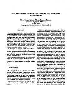
Figure 1: VISTAS simulator at NASA Langley Research Center.

mean(r.getBel(), r.getP l()) 2 · r.getU n()

5 Validation with Aviation Application

P ← R.getConsequent() mean(R.getBel(), R.getP l()) Pconf ← 2 · R.getU n() O ← getObservedOutcome(d) Oconf ← O.getConf idence() Cconf ← C.getConf idence() if (P 6= O) then if (Cconf > T )∧(Oconf > T )∧(Pconf > T )

Next, we present a proof of concept of our framework. Our implementation takes place in the aviation domain, as a contribution to a decision support system, for the identification and reasoning behind anomalous actions in a flight scenario. Specifically, we look at a decision support system whose primary purpose is to assist the pilot with flight missions, with the goal of optimizing safety and general mission success.

5.1 The “Go-Around Decision” Use Case

C.add(createN ewContext(d)) else continue; else C.updateContext(d)

We looked at a scenario where the pilot decides to force a landing in a context where the learned rule prescribes a goaround maneuver. In the situation where a commercial aircraft is unstable below 1000ft on its descent, a flight manual would mandate that the pilot circle the aircraft back, and reattempts the landing. There are certain emergency situations in which the pilot may avoid this prescription (i.e. fire on the aircraft, hijacker, etc). In our proof of concept, we set the fuel level to be low, which would be a realistic scenario that a pilot would chose to abort a go-around to force a landing. The proof of concept ran on a rapid prototyping flight simulator at NASA Langley Research Center in Hampton, VA (see Figure 1). The selected flight scenario for our proof of concept was on the descent of a Boeing 757 into the RenoTahoe International Airport. The interface to the simulator maintained a data recording rate of 50 Hz, with each frame containing 130 data fields corresponding to the flight, running in real-time. That is, the algorithm runs and checks for anomalies as a human is flying the aircraft. Our framework requested data from the simulator interface at a constant rate of roughly 1000ms, which corresponded to a window of time needed for processing. Thus, we define one time step as roughly 1000ms.

The confidence values in lines 14, 16, 17 are extracted from the Dempster-Shafer evidential interval of the respective entities described, and are used to reflect the confidence that the entity in question holds. The value P ⊂ δC in line 13 refers to the prediction that context C will yield P (that is, C =⇒ P ), generated by evaluating each of the implications associated with C, and picking the one with the highest confidence value, and thus the greatest likelihood of occurring. Any data point where the predicted behavioral attribute of C does not correspond with the observed behavioral attribute of C is considered an abnormality. To further distinguish the subgroups of the abnormality points, the algorithm classifies anomalies as all points that occur at a time t where the confidence in the assumed context C is high, the confidence in the implication P is high (that is, the prediction of P), and the confidence in observed implication O is high. All other points in the set of abnormalities are considered outlier points. To further clarify this with an example, lets us consider alternative cases where P 6= O. In the case where the discrepancy P 6= O is observed, and Cconf idence is low, we cannot be sure whether the discrepancy is valid. This is because with a low confidence in the antecedent of the rule C → P , it cannot be validated whether the high confidence on P holds, therefore invalidating the discrepancy. Similarly, with a low confidence on either P or O, it cannot be validated that the discrepancy is occurring.

5.2 Representations Primitive Data Points The simulation generated a broadcast of raw data points that represented the data being generated in the cockpit, describing the current flight running in real-time with a human operator. Each data point contained 130 data fields. The algorithm pinged the simulation broadcast for cockpit data at each iteration of the algorithm (each 1000ms time step). The data

4

Tenth International Workshop Modelling and Reasoning in Context (MRC) – 13.07.2018 – Stockholm, Sweden

points were not only used to inform the anomaly detection portion of the algorithm (line 19), but also for updating the current context assumed by the algorithm and for observing the current action being performed by the pilot.

P∗conf , and O∗conf , respectively, and correspond to lines 17,14 and 16 in Algorithm 1. The confidence value calculated for P∗conf idence is extracted using the DS interval values, whereas the confidence values for C∗conf and O∗conf are calculated using the mean of the mass values on evidence measures supporting their existence.

Context We represent a context with three attributes. The first is a contextual attribute defining a feasibility region, containing the maximum and minimum values (critValMin, critValMax) on each data field within a data point, along with the maximum and minimum deltas values on each field (critDeltaMin, critDeltaMax) within a time window of 50 data points. This characterizes the continuous values of the context by folding data into past values. The second attribute is also a contextual attribute, but this time containing discrete data qualitatively describing the context. A context can contain four discrete values, (STABLE, UNSTABLE, ABOVE1000FT, BELOW1000FT). These discrete values were selected by experts as attributes that are highly relevant to the go-around decision. Finally, each context contains a set of rules, corresponding to implications that should hold in the context, along with Dempster-Shafer intervals to express the confidence of the implication holding in a given context.

5.3

P∗conf = max(

Bel(P ) + P l(B) ), ∀P ⊂ δC∗ 2 · U n(P ) Σm(F ) , F ⊂ φC∗ |φC∗ | Σm(Y ) = , Y ⊂ ΦC∗ |ΦC∗ |

C∗conf = O∗conf

5.4 Results

(8) (9) (10)

In all trials, the algorithm was able to successfully detect the anomaly at the time of occurrence. The algorithm was successful among all human experimenters and participants, which presented variation in flight style, flight trajectories, and flight experience. The nature of the training did have an effect on the number of anomalous features found. The iteration trials captured an average of 8.6 anomalous features, whereas the variation trials captured an average of 2 anomalous features. We found that there was no correlation between the number of anomalous features found and the number of iterations within the iteration trials. We attribute this to the fact that in all iterations of training, the contextual data was the same, so the feasibility region defined by each iteration was the same. We found that with more training iterations, there was a smaller uncertainty for the rules of the normal context. This is consistent with what we expected, since in DST, more iterations provides more evidence supporting the certainty of a rule occurring. Our simulation ran for 100 time steps. The average time step for an anomaly to be detected since the simulation start time was 71.08 seconds, with a minimum time of 57 seconds, and a maximum time of 88 seconds. In each case, the time of detection was identical to the time that the anomaly occurred. The amount of time that it took for the anomaly to be detected was due to human factors. Since the learned context was characterized by being unstable below 1000ft, the anomaly could only occur when these events were happening with a 50% accuracy value, or higher. In all trials, the human subject configured the aircraft to be fully unstable before crossing below the 1000 ft altitude mark, which means that the anomaly generally occurred when the subject crossed the altitude marker. There was no specific reason for the variation in this timing of this event. There was no correlation between the time of the anomaly detection, and the number of anomalous features found. We predicted that the longer it took for the anomaly to be detected, the smaller the number of anomalous features would be found, since there is more time to build up the contextual representation for the learned context. Our trials which were trained with a variation of datasets, rendered a very small number of anomalous features found (2 on average). The features found across all trials were “FUEL WEIGHT LB” and “UPDATE COUNTER” (which correspond to the weight of the fuel present in the aircraft,

Application Specific Instantiation

The proof of concept is run in two segments. First, the system undergoes an initial learning phase to build contextual representations of the Approach phase of flight. Next, the algorithm runs a simulation where the framework is used to detect anomalies in real-time, if and when they occur. Initial Context and Rule Training We trained our system on past flight records where the pilot performed a Go-Around maneuver when he/she found their aircraft in an unstable configuration below 1000 ft on his/her approach. We ran 24 simulations, with trials 1-12 flown by participant A, trials 13-17 flown by participant B, and 18-25 flown by participant C. We removed trails 13, 14, 15 and 21 due to experimental error. A dataset is a prerecorded flight used for training the algorithm, where an aircraft follows commercial aviation protocol by performing a go-around in a context where the aircraft is unstable below 1000ft on its approach. We used 3 datasets (dataset A, dataset B, dataset C). Trials 1-6 were run with only one iteration of training on dataset A, trials 6-9 with two iterations of training on dataset A, and 9-11 with three iterations on dataset A (iteration trials). Trials 12-25 were training with an iterations on each of dataset A, dataset B, and dataset C (variation trials). Training resulted in an implication, C∗ = {U N ST ABLE ∧ BELOW 1000F T } =⇒ GA, (where C∗ is the learned context) that served as a baseline for a ”Normal” prediction when in context C∗ . Using Confidence Values in Simulation Once the initial training had taken place, we began running the simulation. At each time step, the system calculates three values (a confidence value on being in C∗ , the confidence in the a predicted action (from DS intervals), and the confidence in the observed action) which are referred to as C∗conf ,

5

Tenth International Workshop Modelling and Reasoning in Context (MRC) – 13.07.2018 – Stockholm, Sweden

Figure 2: Normal and Anomalous Traffic Data Points

Figure 3: Percentage of Anomalies Found for Each Distribution

and the internal update counter kept by the simulator, respectively). In this case, concluded that the varied training was sufficient enough to narrow down the anomalous feature to only the true cause of the anomaly.

Next, we demonstrate our framework on a traffic dataset containing a much larger number of data points. We chose to use this dataset to show the upward scalability of the framework, working in cases with a large number of data points. Likewise, we validate the framework’s ability to generalize, scaling down to a very simple representation of context.

to determine which of the 5 contexts we are in. For example, with a T Dd value of 4.45, we would be in context C(0,5] , which contains all data points that have a traffic density within the range (0, 5]. For this context, we have T Dd ⊂ φC(0,5] and Sd ⊂ δC(0,5] . We then use these points to calculate our C∗conf O∗conf and P∗conf values. C∗conf was calculated using one of three distribution functions (boolean function, linear function, or normal distribution) based on the range of speeds learned in training. P∗conf was calculated using the DST values associated with the rules (in the same manner as the aviation use case), and O∗conf was calculated using a simple boolean function.

6.1

6.3 Results

6

Algorithm Scalability with Traffic Dataset

Representations

The anomaly points occurred at time steps 1212, 2005, 2283, 2286, and 2290. We ran 3 trials with different distribution functions for determining the confidence of being in a context. Each trial contained 9 runs where we varied the threshold value, stepping up from 0.1 to 0.9. For all 3 trials, the number of detected anomaly points diminished as a function of growing the threshold value. This reflects the algorithms ability to adjust based on how conservative the use case is. For all 3 trials, a threshold value of 0.1 was able to capture all 5 anomalies, with a 0% false positive rate. The drop off rate for the three different confidence value distribution functions for the context varied, but for all three, anomalies were not detected beyond a threshold value of 0.7.

We use the publicly available traffic data at (https://github.com/numenta/NAB). The dataset contains 2380 data points with three fields per point (time, traffic density, and speed). Each data point records the traffic density within an observed frame of space, along with the average speed of the cars passing through the space. Each one of these points serves as a primitive data point. We used a datafile containing 5 human labeled, distance based anomalies as our test dataset (DwithAnomaly ), and the same dataset with the anomalies removed as our training dataset (DwithoutAnomaly ). In the preprocessing step, we trained the system with the DwithoutAnomaly . The data points were split up and used to populate the raw data representation of 5 different contexts, each with a specified range of traffic densities, defining a hard-coded upper and lower bound on the density values (see Figure 2). These traffic density values define the contextual attributes of a context. For each context, there is also an upper and lower bound on speed, which is found through training. These values define a feasibility region for the behavioral attributes of the context. For example, for any data point that has a traffic density reading between 5 and 10, there is an upper bound of 80 mph and a lower bound of 70 mph. These two values together define a feasibility region for the context.

6.2

7 Conclusions and Future Work We created a framework with the goal of being able to detect anomalies with a generalized central algorithm. In our aviation application, we integrated our framework into a complex, human-in-the-loop system running in real-time, where the central algorithm was able to detect anomalies at the time of occurrence in all trials. The detection was invariant across variations in training data, iterations of training data, human participant trials, and across time for anomaly occurrence. In our traffic data application, our algorithm scaled to a larger dataset, where is was able to capture all anomalies with a 0% false positive and false negative rate, at specific threshold values. Varying the threshold values and distributions of the context confidence showed that the the framework can ad-

Application Specific Instantiation

For every data point d processed in simulation, we extracted the traffic density, T Dd , and the speed, Sd . We use T Dd

6

Tenth International Workshop Modelling and Reasoning in Context (MRC) – 13.07.2018 – Stockholm, Sweden

crowded scenes. In Computer Vision and Pattern Recognition (CVPR), pages 1975–1981, Berkley, CA, 2010. IEEE. [Napoli et al., 2015] Nicholas J Napoli, Laura E Barnes, and Kamal Premaratne. Correlation coefficient based template matching: Accounting for uncertainty in selecting the winner. In Information Fusion (Fusion), 2015 18th International Conference on, pages 311–318. IEEE, 2015. [Shafer and others, 1976] Glenn Shafer et al. A Mathematical Theory of Evidence, volume 1. Princeton University Press Princeton, 1976. [Sharma et al., 2016] Manali Sharma, Kamalika Das, Mustafa Bilgic, Bryan Matthews, David Nielsen, and Nikunj Oza. Active learning with rationales for identifying operationally significant anomalies in aviation. In Joint European Conference on Machine Learning and Knowledge Discovery in Databases, pages 209–225. Springer, 2016. [Shon and Moon, 2007] Taeshik Shon and Jongsub Moon. A hybrid machine learning approach to network anomaly detection. 177(18):3799–3821, 2007. [Srivastava et al., 2008] Abhinav Srivastava, Amlan Kundu, Shamik Sural, and Arun Majumdar. Credit card fraud detection using hidden markov model. IEEE Transactions on dependable and secure computing, 5(1):37–48, 2008. [Williams and Scheutz, 2016] Tom Williams and Matthias Scheutz. Resolution of referential ambiguity using dempster-shafer theoretic pragmatics. In AAAI Fall Symposium on AI and HRI. AAAI, 2016.

just to high or low sensitivity use cases, where the detection of anomalies may need to be more or less liberal. The main limitation of our framework is that the feasibility region heuristic for anomaly detection is limited. The linear nature of this heuristic may not be sufficient for all anomaly cases. Some anomalies may only be realized when considering a multifaceted combination of factors [Sharma et al., 2016]. These cases were not considered in our proof of concept. In future work, we plan on using Dempster-Shafer Theoretic intervals on all central elements in the framework, in order to better generalize the method of generating confidence values. We also plan to test the scalability of our algorithm by using it in cases where contexts contain more than two rules, and across more complex domains, which may present more a complex representation of the central elements.

References [Agrawal and Agrawal, 2015] Shikha Agrawal and Jitendra Agrawal. Survey on anomaly detection using data mining techniques. Procedia Computer Science, 60:708–713, 2015. [Agrawal et al., 1993] Rakesh Agrawal, Tomasz Imieli´nski, and Arun Swami. Mining association rules between sets of items in large databases. In Acm sigmod record, volume 22, pages 207–216. ACM, 1993. [Buczak and Guven, 2016] Anna L Buczak and Erhan Guven. A survey of data mining and machine learning methods for cyber security intrusion detection. IEEE Communications Surveys & Tutorials, 18(2):1153–1176, 2016. [Chandola et al., 2009] Varun Chandola, Arindam Banerjee, and Vipin Kumar. Anomaly detection: A survey. ACM computing surveys (CSUR), 41(3):15, 2009. [Dewasurendra et al., 2007] Duminda A Dewasurendra, Peter H Bauer, and Kamal Premaratne. Evidence filtering. IEEE Transactions on Signal Processing, 55(12):5796– 5805, 2007. [Fagin and Halpern, 2013] Ronald Fagin and Joseph Y Halpern. A new approach to updating beliefs. arXiv preprint arXiv:1304.1119, 2013. [Kay, 2007] Rakowsky Uwe Kay. Fundamentals of the dempster-shafer theory and its applications to system safety and reliability modelling. Reliab. Theory Appl, 3:173–185, 2007. [Kuok et al., 1998] Chan Man Kuok, Ada Fu, and Man Hon Wong. Mining fuzzy association rules in databases. ACM Sigmod Record, 27(1):41–46, 1998. [Laptev et al., 2015] Nikolay Laptev, Saeed Amizadeh, and Ian Flint. Generic and scalable framework for automated time-series anomaly detection. In Proceedings of the 21th ACM SIGKDD International Conference on Knowledge Discovery and Data Mining, pages 1939–1947. ACM, 2015. [Mahadevan et al., 2010] Vijay Mahadevan, Weixin Li, Viral Bhalodia, and Nuno Vasconcelos. Anomaly detection in

7