A Framework for Detecting and Diagnosing Anomalies in ... - ITC

RCATool – A Framework for Detecting and Diagnosing Anomalies in Cellular Networks Pierdomenico Fiadino, Alessandro D’Alconzo, Mirko Schiavone, and Pedro Casas Telecommunications Research Center Vienna - FTW {surname}@ftw.at Abstract—The DNS protocol has proved to be a valuable means for identifying and dissecting large-scale anomalies in omnipresent Over The Top (OTT) Internet services. In this paper, we present and evaluate a framework for detecting and diagnosing traffic anomalies via DNS traffic analysis. Detection of such anomalies is achieved by monitoring different DNS-related symptomatic features, flagging a warning as soon as one or more of them show a significant change. The investigation of the root causes for such deviations is done by looking at significant changes in a number of diagnostic features (i.e., device manufacturer and OS, requested host name, error codes, etc.), which convey information directly linked to the potential origins of the detected anomalies. For the purpose of detecting significant changes in the time-series of diagnostic features, we propose two different schemes: the first is based of change point detection applied to the entropy of the considered features, the second considers the full statistical distribution of the traffic features. The proposed solutions are tested and compared using both real and synthetic data from a nationwide mobile ISP, the latter generated from real traffic statistics to resemble the real mobile network traffic. To show the operational value of the proposed framework, we report the results of the diagnosis in two prototypical cases. Keywords—Anomaly Detection; Root Cause Analysis; Network Measurements; Statistical Analysis.

I.

I NTRODUCTION

During the last decade, a plethora of new, heterogeneous Internet-services have become highly popular and omnipresent, imposing new challenges to network operators. The complex provisioning systems used by these services induce continuous changes that impact both operators and customers. Indeed, efficient traffic engineering becomes a moving target for the operator [1], and management of Quality of Experience (QoE) gets more cumbersome, potentially affecting the end customer [3]. Furthermore, due to their traffic characteristics, applications that provide continuous online presence (e.g., messaging services) might severely impact the signaling plane of the network, especially in mobile networks [6]. In such a complex scenario, it is of vital importance to promptly detect and diagnose the occurrence of large scale changes that could result in anomalies for some of the involved stakeholders. In this paper we take a step forward from our previous work [4], where we have initially investigated the problem of diagnosing network traffic anomalies caused by specific devices and applications. Here we propose a more general detection and diagnosis framework, i.e. a Root Cause Analysis (RCA) tool, and cast it to the analysis of Domain Name System (DNS) traffic. The DNS is the core component of the Internet, providing a flexible decoupling of a service’s domain name and the hosting IP addresses. Modern load balancing mechanisms

rely on the diversification of DNS answers to different clusters of users [2], where the Time to Live (TTL) of those answers is usually short, in the order of a few seconds. As a consequence, every time a user tries to access a remote service, it is likely to generate a new DNS query. Based on these observations, anomalies in such services are likely to induce changes in the normal DNS usage patterns. For example, users accessing a temporary unreachable service would generate a new query at every connection retry [7]. Along with the DNS request-response transaction data, our approach assumes the availability of meta-data. In the specific case of traffic originated from a mobile network, these metadata include information related to the end-host (e.g., device manufacturer, Operative System), the access network (e.g, Radio Access Technology – RAT, Access Point Name – APN, IP address of the DNS resolver), and the requested service (e.g., requested Fully Qualified Domain Name – FQDN). Leveraging these DNS data, we extract two sets of features denoted as symptomatic features and diagnostic features. Symptomatic features are defined such that their abrupt change directly relates to the presence of abnormal and potentially harmful events, while diagnostic features shall provide contextual details of the anomalies, pointing to their root causes. Features are further processed to define what we shall refer to as analysis signals. Signals describe the statistical content of features, and allow for abstraction and generalization of the framework’s input definition. For example, a relevant feature used in our framework is the number of DNS requests per observed FQDN in a certain time bin; in this case, a signal associated to this feature could be defined as the mean number of DNS requests, the total number, the full empirical distribution, the entropy, etc. Two signals derived from the same feature might yield completely different detection results: for example, an anomaly could be easily spotted when analyzing the entropy of a certain feature, but not through its mean value. The separation between feature and signal allows to decouple the meaning of an input from the information it exposes for detecting anomalies. The contributions of this paper are as follows: (i) a generic detection and diagnosis framework for Internet service anomalies proposed with two alternative change detection schemes; (ii) a procedure to generate semi-synthetic DNS traffic and to model different types of anomalies observed in real mobile traffic; (iii) an initial evaluation of the proposed framework, considering two different anomaly detection approaches: an entropy, change-detection based anomaly detector, and a distribution-based anomaly detector; as final contribution, (iv) we provide guidelines on how to correlate the traffic

Field Name

Description

Device ID Manufacturer OS APN RAT DNS Server FQDN Error Flag

Anonymized device identifier Device manufacturer Device operating system Access Point Name Radio Access Type IP address of the DNS resolver Fully Qualified Domain Name of remote service Status of the DNS transaction

Table I. Figure 1.

Overview of the detection and diagnosis framework.

feature changes to automatically generate event signatures, classifying as such the root causes of the detected changes. These guidelines form the basis of the automatic diagnosis component of the framework. The remainder of this paper is organized as follows: Sec. II overviews the proposed diagnosis framework. Sec. III describes the two different change detection approaches used to pinpoint changes in the DNS traffic. Sec. IV is devoted to the characterization of the DNS traffic and the generation of synthetic datasets. In Sec. V we discuss the results obtained by applying the framework to two specific types of anomalies, modeled from the real mobile network traffic. Sec. VI provides guidelines for the design of the diagnosis block of the proposed framework. Finally, Sec. VII concludes this work. II.

DNS TICKET INFORMATION ( META - DATA ).

D ETECTION AND D IAGNOSIS F RAMEWORK

In this section we describe a generic framework to detect and diagnose large-scale network traffic anomalies, applied to the analysis of DNS traffic. Fig. 1 sketches an overview of the proposed framework in this application scenario. From DNS tickets we derive two sets of signals denoted as symptomatic signals and diagnostic signals. All signals are checked for significant changes from their reference of “normality”. However, the symptomatic signals are designed such that their changes directly relate to the presence of abnormal and potentially harmful events. On the other hand, changes in the diagnostic signals per-se do not have a negative connotation, but rather ease and guide the interpretation of the anomalous event. In the diagnosis step, deviations of the symptomatic signals are correlated with the subset of simultaneously changing diagnostic signals to provide a comprehensive characterization of the event. We assume that a network monitoring system tracks the DNS traffic at a vantage point in the core of a typical mobile network. A DNS ticket summarizes info related to a DNS query generated by a mobile device, and the reply from the DNS resolvers. The tickets also contain the meta-data listed in Tab. I. These data provide further information about the mobile device (ID, manufacturer, OS), the network settings (APN, RAT, DNS server IP), and the FQDNs of the remote service. Additionally, the Error Flag records the status of the DNS transaction as tracked by the network monitoring system (i.e., successful, time-out, retransmission). As abrupt changes in the number of DNS queries often indicate the presence of application- or device-specific anomalies, the number of DNS queries per unit of time is amenable as symptomatic feature. As for the diagnostic signals, we look

at the distribution of the fields in Tab. I to characterize the subpopulation of devices affected by the anomaly (manufacturer, OS), the remote service involved (FQDN), the network settings (APN, server IP), and finally the possible effect on the DNS infrastructure (Error Flag). In this work we focus exclusively on DNS-related signals. However, the proposed framework is generic enough to operate with different network data sources, such as flow-level or application layer information, which might contribute to further refine the anomaly diagnosis. We leave this for future work. The output of the change detection feds the final Diagnosis block of the framework, whose formal definition is part of our ongoing work. We envision a smart module capable of finding temporal correlations of signals’ changes. The framework should be ultimately able to automatically generate an event fingerprint in correspondence to one or more anomaly symptoms, enriched with diagnostic information. Such a report would provide a valuable basis for supporting the anomaly troubleshooting process. Initial guidelines for the design of this block are sketched in Sec. VI. In this paper we focus on the two fundamental aspects of the proposed framework, namely the definition and extraction of the symptomatic and diagnostic signals, and the design of suitable detection schemes. We address these items in the next section. III.

S IGNALS E XTRACTION AND C HANGE D ETECTION T ECHNIQUES

Let us now formalize the definition of features and signals as considered in the proposed framework, as well as describe the applied change detection techniques. For the generic feature f derived from the DNS tickets, we indicate by fiτ (t) the generic counter observed at the t-th time bin of length τ . For instance, if f represents the number of DNS requests for a FQDN every τ minutes, i ∈ {1, . . . , n(t)} is the i-th requested FQDN, while fiτ (t) counts the number of DNS requests for the i-th FQDN (out of the n(t)), over the t-th time bin. The i-th counter can also be associated to other fields, such as the OS version, the Error Flag value, the number of DNS queries generated by the i-th device, etc. The length of τ defines the timescale of the data aggregation, which in turn defines the timescale of the observable anomalous events. The set of counters F τ (t) = {fiτ (t)} can be used to derive the empirical distribution of the feature f , denoted by Xfτ (t). By properly grouping features, we can obtain aggregated statistics for different “views” on the data. Considering the example above, the FQDN counters can be further grouped to obtain, e.g., 2-nd Level Domain (2LD) or 3rd Level Domain (3LD) counters and statistics. We can also

use the counters for� computing the overall number of DNS requests as N (t) = i fiτ (t). As the following analysis can be done independently of the specific selected time scale, we omit the superscript τ from now on. A. Entropy-based Anomaly Detection Entropy-based anomaly detection is a well-known technique in the literature [8]. Given the empirical distribution Xfτ (t) of a certain feature f , we can compute the normalized entropy as: � 1 H(X) = − x(ω) log x(ω), (1) log(|Ω|) ω∈Ω

where Ω and |Ω| are a discrete probability space and its cardinality, respectively, and x(ω) is the probability of element ω. The entropy of a feature f is a well-suited synthetic index for describing an entire distribution, and in particular, useful for detecting important changes. The first change detection scheme we consider is based on the well-known Exponential Weighted Moving Average (EWMA) algorithm. EWMA weights past observations such that the older ones count less in the determination of the expected current value. For the observed value y(t) at the time bin t, the value predicted by EWMA is calculated as: y˜(t) = λy(t) + (1 − λ)˜ y (t − 1),

(2)

where λ controls the filter memory, that is the weight of the past samples in computing the moving average: the higher λ the higher the weight of the newer samples. Then, the Upper Control Limit (UCL ) and the Lower Control Limit y (t − 1) and (LCL ) are defined as UCL (t) = (1 + σ)˜ LCL (t) = (1 − σ)˜ y (t − 1), respectively, where σ is a slack factor that controls the width of the acceptance region for normality. Finally, the detection algorithm flags an anomaly if y(t) ∈ / [LCL (t), UCL (t)]. Note that by opportunely tuning λ and σ, the EWMA-based detection algorithm becomes able to accommodate for typical daily and weekly patterns of real network traffic. The EWMA-based anomaly detector is applied on the analysis of both symptomatic and diagnostic signals. We consider the total number of DNS requests N (τ ) as symptomatic signal, and the normalized entropy H(X) of the features in Tab. I as diagnostic signals. We refer to this setting as Approach1 in the rest of the paper. B. Distribution-based Anomaly Detection The second anomaly detection scheme relies on the temporal analysis of the entire probability distributions. By that it is particularly suited to cope with anomalies that involve multiple services and/or affect multiple devices at the same time. The considered non-parametric anomaly detection algorithm computes the degree of similarity between the current distribution Xfτ (t) to a set of (anomaly-free) distributions in a dynamic “observation window” W (t), which describe the “normal” behavior. The heuristic used for the construction of the reference set follows a progressive refinement approach that takes into account the structural characteristics of traffic such as time of day variations, presence of pseudo-cyclic weekly patterns, and long term variations. The comparison

between the current distribution Xf (t) and the associated distributions reference set involves the computation of two compound metrics based on a distribution divergence metric L. The first metric, called internal dispersion (or upper bound), is a synthetic indicator defining the maximum distribution deviation that can be accounted to normal statistical fluctuations, therefore it defines acceptance region for the anomaly detection test. The second one, called external dispersion (or average distance), is a synthetic indicator extracted from the set of divergences between the current distribution Xf (t) and those in the reference. The detection test checks if the average distance exceeds the upper bound. As for the distance metric between two distributions p and q, defined over a common discrete probability space Ω, we rely on a symmetrized and normalized version of the Kullback-Leibler (KL)-divergence defined as: � � 1 D(p||q) D(q||p) L(p, q) = , (3) + 2 Hp Hq where D(p||q) is the KL-divergence, defined as � � � p(ω) D(p||q) = . p(ω) log q(ω)

(4)

ω∈Ω

Analogously D(q||p) is the KL-divergence between q and p, and Hp and Hq are the entropy of p and q, respectively. The properties of this metric are extensively discussed in [9]. Notice that using a distribution-based approach is intrinsically more powerful, as it considers the entire distribution of different traffic features, rather than only specific moments of the distributions (e.g., mean-based, variance-based, or percentilebased change detection). By that, it is particularly suited for detecting macroscopic traffic anomalies, that is events that involve multiple services and/or affect multiple devices at the same time. Reporting changing elements: When a change is flagged by the detection algorithm, it also returns the list of the elements ω ∈ Ω that have contributed most to the deviation of the current distribution Xf (t) from the reference of normality. The procedure for identifying the top changing elements easily follows from the eq. (4). Let p be the current distribution, and r the reference distribution computed as by averaging the distributions in the reference set. We define δ(ω), the drift value of ω, as follows: δ(ω) = p(ω)log

p(ω) , r(ω)

(5)

which intuitively represents the contribution of the element ω to the overall external dispersion. At every iteration, the algorithm ranks the changing elements by value. In order to get a compact representation, the algorithm reports only the top-k elements accounting for r% of the overall change. From our experience, r = 50% provides best results, that is the algorithm returns only the few elements really responsible for the distribution change, and discharge those resulting from random statistical fluctuations. Notice that, reporting the list of the most significant variables is a key feature for the diagnosis process. Indeed, it allows having fine-grained information on the root causes of the distribution change, in addition to the mere change notification.

Self-adaptation to long-lasting changes: The algorithm originally proposed in [9] has been designed with the intent of detecting large-scale security or performance anomalies. It is expected that these anomalies are transitory and have a limited duration. Consequently, the mechanism for updating the observation window is designed such that W (t) is frozen till the anomaly is over. However, we now apply the same algorithm to the detection of changes in the diagnostic signals, which may exhibit long-lasting anomalies corresponding to working point changes. For example, let us consider a popular service that updates its naming scheme, heavily impacting the distribution of counters per FQDNs. In this case W (t) remains locked (i.e., it is not shifted forward till the anomaly is over), and the algorithm keeps indefinitely flagging warnings, making it unusable. To cope with this limitation when facing long-lasting changes in the diagnostic signals, we enhanced the updating mechanism of the observation window such that it dynamically adjusts the number of valid (i.e., non anomalous) distributions in it. Let us indicate by m and L0 (t) = mτ the number of valid distributions and the length of the W (t) respectively, when W (t) contains no anomalous distributions. As soon as an anomaly is detected, the length of observation window increases by one to L1 (t) = (m + 1)τ , whereas the number of valid distributions remains m. When m anomalies are detected in a row, the observation window length becomes Lm (t) = 2mτ , and we switch to a soft test state where we allow anomalous distributions in the observation window to enter the reference-set. In this state, if the anomalous distributions are consistent enough (i.e., refer to the same event), and the anomaly lasts longer than m, then they are likely selected as new reference for normality and the test turns negative. From this moment on, every time the test is negative W (t) is reduced such that L(t + 1) = L(t) − 2τ , till it gets back to L0 . At that point the algorithm exits the soft test state. Notice that in this way the algorithm accommodates to the new working point after a transitory phase of mτ during which the algorithm keeps flagging an anomaly. When the distribution-based anomaly detector is used, we consider as symptomatic signal the distribution of number of devices across query counts, i.e., counting how many devices execute a given number of requests within each time bin. In fact, perturbations in this distribution indicate that a device sub-population deviates from the usual DNS traffic patterns, thus pointing to potential anomalies. The diagnostic signals are instead the distributions of query count across the variables of the features in Tab. I. We refer to this detection and diagnosis scheme as Approach2 in the following. IV.

DNS T RAFFIC C HARACTERIZATION AND A NOMALY M ODELING

We evaluated the proposed framework for longer than six months in 2014 with traffic from the operational cellular network of a nationwide European operator. The extensive experimentation allowed us to collect results in a number of paradigmatic case-studies exposing features and limitations of the framework. Still, the number of DNS traffic anomalies observed in the corresponding period was relatively low, limiting as such the chances of performing a complete performance analysis of the framework by relying exclusively on real traffic.

1

0.8

0.6

0.4 users queries 0.2 Tue

Wed

Thu

Fri

Sat

Sun

Mon

time [bin=30min]

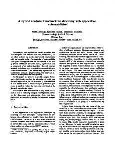
Figure 2. Daily trend of the number of active users and total DNS query count in the semi-synthetic dataset.

In principle, one could resort to test traces obtained in a controlled environment (laboratory) or by simulations, but these approaches would miss the complexity and heterogeneity of the real traffic. To bypass this hurdle, we adopted a methodology based on semi-synthetic data, derived from real traffic traces as suggested in [11]. Such an approach does not only allows to extensively analyze the performance of the framework with a large number of synthetic, yet statistically relevant anomalies, but also permits to protect the operator’s business sensitive information, as neither real data traces nor real anomalies are exposed. Next we explain the procedures for both generating a semi-synthetic background DNS traffic, as well as for modeling the DNS-related anomalies for replicating them. A. Semi-synthetic Dataset Construction The procedure for constructing the semi-synthetic dataset is conceived with the objective of maintaining as much as possible the structural characteristics of the real, normal operation (i.e., anomaly-free) traffic, while eliminating possible (unknown) anomalies present in real traces. Exploring real traces, we observed that the traffic yields some fundamental temporal characteristics. In particular, the traffic is non-stationary due to time-of-day variations. This effect is not limited to the number of active devices and the number of DNS queries, but rather applies to the entire distribution. Distribution variations depend on the change of the applications and terminals mix, which in turn induce modifications in the DNS request generation patterns. Furthermore, we found that, besides a strong 24hours seasonality, the DNS traffic exhibits a weekly pseudocyclicity with marked differences between working days and weekends/festivities [7]. Finally, traffic remains pretty similar at the same time of day across days of the same type. The first step of the construction procedure consists of manually labeling and removing possible anomalous events. However, as the complete ground truth is unknown in real traffic, we cannot completely rely on individual labeling of alarms. Therefore, we have to accept that minor anomalies may go undetected if their effect is comparable with purely

DNS requests

1

0.8

0.7

CDF

0.6

0.5

0.4

0.3

���

���

���

���

���

Anomalous distributions ���

���

10

1

2

10 Query count

10

3

10

���� ���� ���� ���� ���� ���� ���� ���� ���� ����� ����� ����� ����� ����� ����� ����� ����� ����� ����� ����� ����� ����� ����� �����

���

0.2

0.1 0 10

�

���

0.9

�

�

1:00 2:00 3:00 4:00 5:00 6:00 7:00 8:00 9:00 10:00 11:00 12:00 13:00 14:00 15:00 16:00 17:00 18:00 19:00 20:00 21:00 22:00 23:00 24:00

4

��� � � ��

��

�

�

�� �����������

��

�

��

�

Figure 3. Hourly trend of the distribution of number of devices across query count over one day of the semi-synthetic dataset.

Figure 4. Hourly trend of the distribution of number of devices across query count over the first day of the E2 anomaly.

random fluctuations. Then, the dataset is transformed to eliminate possible residual (unknown) anomalies present in the real traffic, while preserving the above mentioned structural characteristics. The transformation procedure is described as follows.

In other words, all W-days in the new dataset share the same (synthetic) aggregate daily profile. Same applies to Fdays. Note however that the synthetic dataset retains the most important characteristics of the real process. In the first place, it keeps the time-of-day variations of the number of active devices (see Fig. 2). However, the total number of queries at time k changes as permuted devices issue (in general) different amount of DNS queries. Secondly, the semi-synthetic dataset maintains the differentiation between the two classes of W- and F- days, although it eliminates any differentiation within each class (e.g., between Saturday and Sunday). Thirdly, it keeps the differentiation between distributions for different time-of-day. This is clear from Fig. 3, which shows the hourly Cumulative Distribution Functions (CDFs) of the number of devices across query count during one day of the semi-synthetic dataset. The result of the procedure is an anomaly-free DNS dataset structurally similar to the real trace.

Lets consider a real dataset spanning a measurement period of a few weeks, for a total of m consecutive one-day intervals (e.g., m = 28 in our case). Each one-day period starts and ends at 4:00 am local time: this is the time-of-day where the number of active devices reaches its minimum (considering a single time-zone). Denote by mW and mF the number of working and festivity (W- and F-) days, respectively, in the real dataset (e.g., mF = 8 and mW = 20), and by K the total number of 1-min timebins (K = 28·24·60 = 40320). For each device i consider the vector di ≡ {cτi 0 (k), k = 1, 2, . . . , K} at the minimum timescale (τ0 = 1 minute) across the whole real trace duration, where each element cτi 0 (k) is the list of the DNS tickets related to device i at time k. For those timebins where device i is inactive, the corresponding element in di is empty. We now divide this vector into m blocks, each one corresponding to a single one-day interval. Each block is classified as W- or F-block based on the calendar day. At this point we apply a random scrambling within the W class: each W-block element of di is randomly relocated at the same time position selected among all W-days. The same scrambling is applied independently to the F-blocks. In this � i where the position of the way we obtain a new vector d blocks has been scrambled, separately for W- and F-blocks, but the time location and the F/W intervals have been maintained. � i we can derive a Finally, from the set of scrambled vectors d new set of distributions for each timebin k and timescale τ , for all the considered traffic features. The dataset obtained in this way retains certain characteristics of the real dataset, while others are eliminated. The most important change is that the random scrambling of the � i results in the homogenization individual components di → d of the individual daily profiles — separately for W- and Fdays. This eliminates any residual local anomaly by spreading it out across all one-day intervals of the same F/W type.

B. Construction of Synthetic Anomalies During six months of experimentation we encountered a few recurring large-scale DNS traffic anomalies. Investigating these events we found some common traits and we conceived a procedure for reproducing them along with their most relevant characteristics. In particular, we identified two exemplary event types (E1 and E2 from now). In both the cases, we model an outage of an Internet service for a specific sub-population of devices, which react by repeatedly and constantly issuing DNS queries to resolve the requested service throughout the anomaly. Involved devices are identified by fixing a specific OS (with its different versions). Moreover, we aim at modeling the correlation between the selected sub-population and the unreachable service. Therefore, we separately rank the 2LDs of the FQDNs for anomalous and background traffic, and select the most popular 2LD of the former that is not in the latter. The event of type E1 models the case of a short lived (i.e., hours) high intensity anomaly (e.g., 10% of devices repeating a request every few seconds), where all the involved devices are produced by a single manufacturer and run the same OS. In this case, the number of involved terminals and the overall

Table II.

E1 9:00 1h 10% 5 sec single popular single (with sub-versions) +5% timeout top-2LD for involved devices

E2 13:00 2 days 5% 180 sec multiple single (with sub-versions) — top-2LD for involvede devices

0.70 normalized entropy

Type Start time t1 Duration d Involved devices D Back-off time Manufacturer OS Error flag FQDN

C HARACTERISTICS OF THE ANOMALOUS DNS TRAFFIC FOR TYPE E1 AND E2 .

0.60 0.50 0.40 manuf. error_code OS FQDN

0.30 0.20 0.10 00:00

04:00

08:00

12:00

16:00

1 0.9 0.8 0.7 0.6 0.5 0.4 0.3 0.2 00:00

Figure 6. Normalized entropy of diagnostic features in event type E1 . All signals are clearly altered (spikes and notches) during the event.

query count spikes

2

04:00

08:00

12:00

16:00

ENKLd * 103

number of DNS queries

time [bin=5min]

avg. distance upper bound warnings

1

time [bin=5min]

Figure 5. EWMA change point detector applied to symptomatic signal (query count) in event type E1 . The event is highlighted in the gray area. The red dots marked as spikes correspond to the alarms flagged by the detector.

0 00:00

04:00

08:00

12:00

16:00

time [bin=5min]

Figure 7. Output of the distribution-based detector for the symptomatic signal (number of devices across query count), in E1 type event.

number of additional queries is such to overload the local DNS servers. The latter effect is modeled by increasing the number of time-out codes in the Error Flag field. The event of type E2 models a long lasting (i.e., days) low-intensity anomaly (e.g., 5% of devices repeating requests every few minutes). Differently from the previous case, the involved terminals are produced by multiple manufacturers, even if they share the same OS. Given the low-intensity, we did not introduce a modification in the distribution of the Error Flag. Fig. 4 shows the changes in the distribution of number of devices across query counts introduced by this event (cfr. Fig. 3). Note that although E2 type anomalies are of relatively low intensity, their identification is important as, in our experience, they may lead to problems on the signaling plane, such as resources starvation at the radio access. Tab. II summarizes the characteristics of the two event types and the actual values used for generating the anomalous ticket dataset in the experiments discussed in Sec. V. To illustrate the anomaly generation procedure, we consider an event of type E1 of duration d = 1h, starting at t1 = 9 : 00. Starting from t1 at each time-bin, D = 10% of all the active terminals are randomly extracted from the semi-synthetic background traffic, such that the OS is the selected one and the manufacturer is always the same. For each involved terminal, we generate one additional DNS ticket every 5 seconds, which are then added to the semi-synthetic dataset. The FQDN in these tickets is randomly chosen among the domains in the 2LD identified as explained above. Finally, the Error Flag is changed to time-out in 5% of the overall DNS tickets, so as to model the resolver overload. The last step consists of mangling both the anomalous and the background traffic.

The procedure for generating type E2 is analogous, but differs in the selection of the anomalous terminals (same OS, but not necessarily same manufacturer). The Error Flag is not changed. V.

E VALUATION AND RESULTS

In this section we present the results on the performance evaluation of the framework in terms of detection and diagnosis capabilities, for the case of the aforementioned anomalies of type E1 and E2 . For each type of anomaly, we report the results obtained by each of the two proposed detection approaches. Reported results refer to optimal parameter settings in terms of detection capabilities and number of false positives. A. Analysis of Event Type E1 As described in Sec. IV, the first event is characterized by a short duration (1 hour) and a high intensity, as it involves a large population of devices (10%) coming from the same popular manufacturer and running one specific OS. The evaluation is performed at a τ = 5 minutes time scale. Approach1. Fig. 5 shows the time-series of the DNS query count, used as symptomatic signal. The gray area highlights the event time span, from 9am to 10am. The increase on the number of DNS queries is clearly visible, resulting in about the double of queries as observed in normal operation conditions at that time of the day. The red points in the figure indicate the deviations flagged by the EWMA algorithm. The entropy trend of the diagnostic features is depicted in Fig. 6. Given the high intensity of the event, marked variations are

60 40 20 04:00

08:00

12:00

16:00

time [bin=5min]

(a) FQDN

20 0 00:00

04:00

08:00

12:00

16:00

30 20 10 0 00:00

04:00

time [bin=5min]

08:00

12:00

10 0 00:00

16:00

avg. distance upper bound warnings

20

04:00

time [bin=5min]

(b) Error Flag

08:00

12:00

16:00

time [bin=5min]

(c) Manufacturer

(d) OS

visible in all the diagnostic signals. In fact, the fraction of DNS queries generated by devices with a specific manufacturer and OS changes during the event, hence the entropy of the respective dimensions exhibit a sharp decrease. Similarly, the FQDN entropy signal decreases, since the affected devices repeatedly try to contact a specific service. On the contrary, the Error Flag diagnostic signal shows a significant increase. In fact, the increased share of time-outed queries perturbs the distribution else concentrated around the successful value, with a consequent spike in the entropy value. The notches and spikes in the entropy, as well as in the query count, are easily detected by the EWMA algorithm. Approach2. Fig. 7 shows the output of the distributionbased detector: the yellow curve represents the average distance between the distribution of the number of users per query count and the distributions in the reference set, while the blue dashed curve is the upper bound for acceptability. As in the previous case the duration of the event E1 is highlighted in gray. The timebins where the average distance is above the upper bound are marked with red points. The figure shows that the distribution deviations are correctly detected. The same applies for the diagnostic signals as depicted in Fig. 8, showing marked changes in the FQDN, Error Flag, Manufactuer, and OS distributions during the event. Summarizing the performance of both detectors for analyzing anomalies of type E1 , both approaches allow to accurately detect the changes on the symptomatic signal, as well as on the diagnostic signals. The changes on all signals are simultaneously detected, providing a reliable input to the diagnosis step. B. Analysis of Event Type E2 Differently from E1 , the type E2 anomaly involves a smaller population of devices (5%) running an OS pre-installed by a number of different manufacturers. Similarly to the previous case, the affected terminals continuously try to recontact the servers hosting an unreachable service. Because of the low intensity and the longer duration of the event, the analysis is performed at a τ = 30 minutes time scale. Approach1. Fig. 9 depicts the time-series of the query count during a period of 3 days, which includes the anomalous event, starting at 1pm of the first day and lasting till 11am of the third day. The counter shows a slight increase during the anomaly, but the EWMA detection algorithm only flags changes at the beginning, and is not able to track the anomaly during its complete time span. Fig. 10 plots the trend of the diagnostic signals. Only the FQDN entropy exhibits evident changes during the night-time, when the increased number of requests for the affected service stems out from the background night traffic. For the rest of the diagnostic signals, it is hard

number of DNS queries

Output of the distribution-based detector for the diagnostic signals in E1 type event. All the signals exhibit distribution changes during the event. 1 0.9 0.8 0.7 0.6 0.5 0.4

spikes

query count 00:00

12:00

00:00

12:00

00:00

12:00

time [bin=30min]

Figure 9. EWMA change point detector applied to symptomatic signal (query count) in event type E2 . The event is highlighted in the gray area. The red dots marked as spikes correspond to the alarms flagged by the detector.

0.60 normalized entropy

Figure 8.

40

30

avg. distance upper bound warnings

40

0.55 0.50 0.45

manuf. error_code OS FQDN

0.40 0.35

00:00

12:00

00:00

12:00

00:00

12:00

time [bin=30min]

Figure 10. Normalized entropy of diagnostic features in E2 type event. No clear evidence of the underlying event, with the exceptions of two notches in the FQDN signal. 30.0 25.0 ENKLd * 103

0 00:00

50

avg. distance upper bound warnings

60

ENKLd * 103

80

ENKLd * 103

ENKLd * 103

80

avg. distance upper bound warnings

100

ENKLd * 103

120

20.0

avg. distance up. bound warnings

15.0 10.0 5.0 0.0

00:00

12:00

00:00

12:00

00:00

12:00

time [bin=30min]

Figure 11. Output of the distribution-bases detection on the symptomatic signal (number of users across query count), in E2 type event.

to claim that the small, low-speed observed changes could be detected, specially as they look very similar to the patterns observed during normal operation. Indeed, the EWMA algorithm fails to track the full dynamics of the event. Regarding the OS signal, the changes in the distribution induced by E2 are not sufficient to alter the entropy signal. We recall that E2 does not affect the Error Flag signal by design.

2

60 40 20 0

2

avg. distance upper bound warnings

2 1 0

00:00

12:00

00:00

12:00

time [bin=30min]

(a) FQDN

00:00

12:00

0

00:00

12:00

00:00

12:00

00:00

12:00

time [bin=30min]

(b) Error Flag

45 40 35 30 25 20 15 10 5

35

avg. distance upper bound warnings

30 ENKLd * 103

3

avg. distance upper bound warnings

ENKLd * 103

80

ENKLd * 103

ENKLd * 103

100

25

avg. distance upper bound warnings

20 15 10 5

00:00

12:00

00:00

12:00

00:00

time [bin=30min]

(c) Manufacturer

12:00

0

00:00

12:00

00:00

12:00

00:00

12:00

time [bin=30min]

(d) OS

Figure 12. Output of the distribution-based analysis for the diagnostic signals in E2 type event. Distributions of FQDN and OS exhibit changes during the event, while manufacturer and Error Flag are unaffected.

Approach2. Contrarily to the previous case, the distribution-based approach detects low-intensity anomalies involving multiple devices. Fig. 11 plots the output of distribution-based algorithm for the symptomatic signal. The average distance (yellow curve) flags changes in the distributions of the number of devices across query, which correspond to deviations in the CDFs shown in Fig. 4. Therefore, the approach is able to capture and detect the entire dynamics of the event. The distance between the two curves is more marked during the night hours, when the number of DNS queries related to the anomaly are statistically more relevant, cfr. Fig. 4. The output of the distribution-based detector applied to the diagnostic signals is shown in Fig. 12. The FQDN signal output, depicted in Fig. 12(a), is correlated with the symptomatic signal: the plot reports a sequence of drifts from the reference set highlighting the whole span of the event. As in E2 there is no anomalous behavior on the Error Flag distribution, a correct functioning of the detector would result in no alarms for this signal, which is exactly depicted in Fig. 12(b). Fig. 12(c) shows that also the manufacturer dimension is not involved, while in Fig. 12(d) there are evidences of the OS-related nature of the anomaly. In conclusion, the experiments show that lower intensity anomalies are not correctly captured by the Approach1, as the entropy is a too coarse metric, failing to reveal the effects of this type of anomalies. This limitation calls for the adoption of a distribution-based approach, which is perfectly suited for both scenarios. VI.

T OWARDS AUTOMATIC D IAGNOSIS

The experimental results of the previous section show the advantage of using the distribution-based change detection approach in the proposed framework. It not only performs better in presence of low-intensity anomalies, but also returns the single distribution elements that cause the changes. The latter information are critical in the diagnosis phase, for the purpose of defining the event signature, as we show next. From now on, we consider the Approach2 as the adopted change detection scheme for both the symptomatic and the diagnostic signals. In this section, we provide guidelines for the design of the diagnosis module (cfr. Fig. 1), derived from the lessons learned from the experimentation. Specifically, we cover two aspects: (i) the definition of a state machine to handle change detection outputs in a state-full manner, (ii) the correlation of the signal changes for the definition of the event signature. A. Change Detection: from State-less to State-full The different instances of the change detection module notify the occurrence of significant modifications detected on

Figure 13. State machine of change detection output. fr is the fraction of change notification in the shift register, th is the state transition threshold. Each symptomatic and diagnostic signal has its dedicated state machine.

the corresponding (symptomatic or diagnostic) signal, along with the elements which contribute the most to the change (cfr. Fig. 1). The notification is done independently at each iteration in a state-less fashion. However, the detectors output may flip from anomalous and normal during the same event, depending on the algorithm sensitivity and on the anomaly intensity. The first task of the diagnosis module is to consolidate the changes referring to the same event. This is done, independently for each signal, by means of a finite state machine. The finite state machine, depicted in Fig. 13, consists of three states, namely Normal, Warning and Anomaly. The state transitions depend on the number of change notifications in a shift register containing the last ns outputs of the detector. We indicate by fr the fraction of change notification in the register. The initial state (Normal) corresponds to fr = 0. As soon as the first change is detected (i.e., the event starts), the signal state switches to Warning (fr > 0). The signal remains in the same state, till a sufficient number of changes has been detected. State transitions depend on a threshold th: when fr > th , the signal enters the Anomaly state. B. Correlation of Signals for Generation of Signatures The main purpose of the diagnosis module is to temporarily correlate symptomatic and diagnostic signals: in a nutshell, by locating those diagnostic signals which show a change at the same time of the detected anomaly, one gets a more targeted and specific indication of which features might be causing the anomaly. This objective is achieved by means of event signatures. Recall from Sec. II, that symptomatic signals are used as evidence of anomalous behavior, while diagnostic signals provide additional information for the diagnosis and the event. When a symptom appears (i.e., the corresponding signal switches to Warning or Anomaly state), a new event signature is instantiated. The signature is enriched with the diagnostic information provided by the other signals: list of changing signals, including the lists of the most relevant changing elements (cfr. Sec. III). The changing elements δ(ω) have a sign, depending on whether their share in the distribution is increasing or decreasing. An example of an event signature is reported below:

symptom diagnostic diagnostic diagnostic

query_per_user manufacturer OS FQDN

time-bin 30m start_warn 2015-02-14 start_alarm 2015-02-14 end_alarm 2015-02-14 end_warn 2015-02-14

[10,+][1,-] [Pineapple,+] [youOS_v2.1,+] [youcloud.com,+]

12:00:00 13:00:00 17:30:00 18:00:00

That is, a change in the symptomatic signal distribution of query per user has been detected starting at start_warn due to an increase in the number of terminals issuing 10 queries, and a decrease of terminals issuing 1 query, in every 30min time-bin. The event signature indicates that the devices produced by Pineapple, equipped with version 2.1 of the operative system youOS increased their shares of queries in the respective distributions. Also, the event signature indicates that the number of queries for the FQDN youcloud.com has increased. This shall be the typical signature generated for an anomaly of type E1 (cfr. Sec. IV) lasting six hours, where involved terminals retry to access youcloud.com every 5 minutes (10 requests every 30 minutes). Notice that the event signature describes the event throughout its entire duration. Given an event, this one is considered as closed if the symptomatic signals are back to Normal state, or if there is a change in the signature (i.e., an event change); in the latter case, a new event is initialized. A change in the signature could be caused by either a change in the involved signals (i.e., a new diagnostic signal enters Warning state, or a signal that was in Warning/Anomaly goes back to Normal), or in the list of changing elements of one of the diagnostic signals (e.g., a new FQDN appears, disappears, or changes sign).

anomalies occuring at the same time, involving an even smaller user population. Given the general lack of large-scale ground-truth datasets to test the performance of systems like ours, we developed an approach to generate semi-synthetic data, derived from real traffic traces. We believe that this is also a main contribution of our work, as it would help to owners of real data to make such datasets available for the research community. Last but not least, we have presented a preliminary draft of an automatic diagnosis module capable of correlating changes in symptomatic signals and automatically generate event fingerprints. The operational value of such an automatic fingerprinting approach is paramount, as it could potentially result in a dramatical reduction of the time spent by network operators in diagnosing unexpected events. Our on-going work consists in extending the framework with heterogeneous data sources to enrich the diagnosis of anomalies with additional signals. We are also working to improve the diagnosis module, and plan a large-scale performance assessment, relying both on operational data, as well as on the synthetic traffic and anomalies’ generator proposed in this paper. ACKNOWLEDGMENTS The research leading to these results has received funding from the European Union under the FP7 Grant Agreement n. 318627, “mPlane”. R EFERENCES [1] [2]

VII.

C ONCLUSIONS

The DNS protocol has proved to be a valuable means for identifying and dissecting large-scale anomalies in omnipresent Over The Top (OTT) Internet services. In this paper we have presented a preliminary study on a framework for automatic detection and diagnosis of large scale Internet anomalies based on the analysis of DNS traffic. Its key idea is to apply a change detection algorithm to a set of meaningful signals extracted from network measurements, and then correlate those signals which show similar abnormal behavior on a similar timespan. To this extent, we have thoroughly tested two different detection schemes both on real network traces and semisynthetic datasets. Our preliminary results unveiled the limitations of using simple change point detection algorithms in the case of low intensity anomalies that involve relatively small sub-populations of users. From our experience, this type of anomalies are frequent in operational mobile networks, and still far from being innocuous (cfr. problems on the signaling plane). To overcome this limitation, we have presented a more complex change detection scheme that relies on the entire probability distribution of the monitored signals rather than the entropy values. Using this detection approach, the system is able to cope with anomalies that involve multiple services and/or affect multiple devices at the same time. Still, we are investiganting the behavior of the two detectors in case of multiple

[3]

[4] [5] [6] [7] [8] [9]

[10] [11]

P. Fiadino, A. D’Alconzo, P. Casas, “Characterizing Web Services Provisioning via CDNs: The Case of Facebook”, in TRAC, 2014. P. Membrey, E. Plugge, D. Hows, “Practical Load Balancing: Ride the Performance Tiger”, APRESS, 2012. P. Casas, A. D’Alconzo, P. Fiadino, A, B¨ar, A. Finamore, T. Zseby, “When YouTube doesn’t Work – Analysis of QoE-relevant Degradation in Google CDN Traffic”, IEEE Transactions on Network and Service Managemen, vol. 11, no. 4, 2014. M. Schiavone, P. Romirer-Maierhofer, P. Fiadino, P. Casas, “Diagnosing Device-Specific Anomalies in Cellular Networks”, in ACM CoNEXT Student Workshop, 2014. P. Fiadino, A. D’Alconzo, A. B¨ar, A. Finamore, P. Casas, “On the Detection of Network Traffic Anomalies in Content Delivery Network Services”, in ITC, 2014. A. Aucinas, N. Vallina-Rodriguez, Y. Grunenberger, V. Erramilli, K. Papagiannaki, J. Crowcroft, D. Wetherall, “Staying Online While Mobile: The Hidden Costs”, in ACM CoNEXT, 2013. P. Romirer-Maierhofer, M. Schiavone, A. D’Alconzo, “Device-specific Traffic Characterization for Root Cause Analysis in Cellular Networks”, in TMA, 2015. G. Nychis, V. Sekar, D. G. Andersen, H. Kim, H. Zhang, “An Empirical Evaluation of Entropy-based Traffic Anomaly Detection”, in ACM IMC, 2008. A. D’Alconzo, A. Coluccia, P. Romirer-Maierhofer, “Distribution-based Anomaly Detection in 3G Mobile Networks: from Theory to Practice”, International Journal of Network Management, vol. 20, John Wiley & Sons, 2010. A. Lakhina, M. Crovella, C. Diot, “Mining Anomalies using Traffic Feature Distributions”, in ACM SIGCOMM, 2005. H. Ringberg, M. Roughan, J. Rexford, “The need for simulation in evaluating anomaly detectors”, in ACM SIGCOMM Computer Communications Review, vol. 38, 2008.