A Generalized Process for Optimal Threshold Setting in HUMS Eric Bechhoefer Goodrich Fuels and Utility Systems Vergennes, VT 05491 802-877-4875
[email protected] Andreas P.F. Bernhard Sikorsky Aircraft Corporation Stratford CT 06615 203-386-4323
[email protected] Abstract— Monitoring the health of a helicopter drive train enhances flight safety and reduces operating costs. Health and Usage Management Systems (HUMS) monitor the drive train by using accelerometers to measure component vibration. Algorithms process the time domain vibration data into various condition indicators (CI), which are used to determine component health via thresholding. 1 2
decision rule for detecting a component which is no longer nominal. The normalized distance distribution is a function of the component CI sample statistic. Procedures are developed to calculate the unbiased statistic: covariance for Rayleigh based CIs and mean value/covariance for Gaussian based CIs. In the cases where the population of components is not nominal (e.g. mass imbalances which violate the Rayleigh assumption) tools are presented to control this. For gear, normalizing transforms can be used to ensure the CIs are more Gaussian. Example data from utility helicopters are given.
For the rotating machinery, a standard set of CI are shaft order one, two and three (i.e. 1, 2 or 3 times the shaft RPM). Shaft order one (SO1) is indicative of an unbalance, where as higher shaft order can be used to detect a bent shaft or misalignment condition. In the case of bearings, CIs are envelope spectrum or cepstrum analysis of the ball, cage, inner race and outer race frequencies. There are a number of standard CI used for gear analysis, such as line elimination and resynthesis, side band modulation, gear misalignment, etc.
TABLE OF CONTENTS 1. INTRODUCTION ..................................................... 1 2. THE NAKAGAMI DISTRIBUTION ........................... 3 3. HI ALGORITHM FOR RAYLEIGH BASED CIS ....... 3 4. HI ALGORITHM FOR GAUSSIAN BASED CIS ........ 5 5. SYSTEM ENGINEERING CONSIDERATIONS ........... 6 5. CONCLUSION ......................................................... 7 6. NOTES ON RAYLEIGH DISTRIBUTION .................. 7 REFERENCES............................................................. 8 BIOGRAPHY .............................................................. 8
In general, some method is used to set thresholds for these CIs: when the threshold is exceeded, maintenance is recommended. The HUMS system must balance the risk of setting the threshold too high such that a component may fail in flight versus the risk of setting the threshold too low, which results in additional maintenance cost. This paper covers a generalized process of optimally setting threshold for CI and fusing the information into an Health Indicator.
1. INTRODUCTION Health and Usage Monitoring Systems (HUMS) have been proven to be indispensable in improving aircraft readiness and reduced maintenance cost. There is a consensus in the helicopter community as what a number of functions do, such as: Usage, Rotor Track and Balance, Exceedance Monitoring and Regime Recognition. But in the case of mechanical diagnostics (MD), there are at least two paradigms for the evaluation of component condition. The first paradigm will be identified as CI based thresholding, and the second paradigm will be called Health Index (HI) based thresholding.
It can be shown that the distributions of CI for shaft magnitude and bearing envelop energy are Rayleigh distribution. The normalized distance functions for these CIs are a Nakagami distribution with µ (shape parameter) of n (number of CI) and Ω (scale parameter) of 2 x 1/(2-π/2) x µ. For gear CIs, which are considered as Gaussian, the normalized distance function is again Nakagami, but with a µ of n/2 and Ω of n. Given the theoretical µ and Ω, a threshold for any set of CI can be generated resulting in system probability of false alarm (PFA). This is an optimal 1
In most HUMS systems, a vibration signature is processed into a number set of condition indicators (CI). For many
1-4244-0525-4/07/$20.00 ©2007 IEEE. 2 IEEEAC paper #1142, Version 1, Updated October 16, 2006 1
1
components, the CI has physical meaning. As an example, shaft order 1 (SO1) is the magnitude of the shaft vibration in inches per second associated with 1 x RPM. Other CIs’ have limited physical meaning, such as gear distributed fault.
unique threshold. In the given example, there would be 25x3 + 27x6 + 65x5 or 562 threshold values. Further, consider the case in which the thresholds have been set statistically, say with a rule in which an alert or exceedance message is generated when a CI is three standard deviations (one assumes here that the distribution of the CI are Gaussian, which is not the case for shaft and bearing CIs).
In the first paradigm, these CI can be viewed and trended on a ground station. In some cases, the original equipment manufacture will supply limits to the components. On the UH-60 helicopter, SO1 limits are given for the engine input drive shaft. In most cases, there are no known limits and a statistical procedure is used (e.g. 3 standard deviations above the mean value) to trigger maintenance.
Using 3 standard deviations, there is 0.0013 probability that any nominal (say good) CI will report an alert (e.g. a false alarm). In one respect, an error on the order of 10-3 seems acceptable. However, consider that each trial (all 562) has a probability of 0.0013, and that this occurs perhaps eight times per hour (e.g. eight acquisitions per hours) giving a total of 4496 trails. With this large number of trails, what is the probability of not generating a false alarm. In one trial, it is simply: p =(1-0.0013)1 = 0.9987. In 562, it is: p = (10.0013)562 = 0.4674 or a probability of drive train false alarm of 0.5326 per acquisition. The rate per hour is then q = 1-(1-0.0013)562x8 = 0.997 or almost 1 per flight hour.
CI Based Thresholding Consider the system engineering of a HUMS designed around this paradigm. Each component has a number of failure modes, and ostensible, a number of CI to detect those failure mode. In the case of shaft (ref 1), there is at least 3 failures modes: Fault Type
Frequency of Dominate Vibration
Out of Balance
1 x RPM (SO1)
Misalignment bent shaft Mechanical Looseness
and
In actuality, this false alarm rate would be higher, because the CI for shaft and bearing, being based on magnitudes, are Rayleigh distributed (ref 2) which are heavily tailed. The false alarm rate using 3 standard deviations for a Rayleigh distribution is 0.0056. In this case, one would expect q =1 (1-0.0056)400 = 0.826 PFA for shaft and bearing per acquisition alone (see Notes on Rayleigh Distribution).
Usually SO1, Often 2 x RPM (SO2) and 3 x RPM (SO3) 2 x RPM (SO2)
HI Based Thresholding In HI based thresholding, the CIs for a given component are fused into one HI. Formally, the HI is a function of distributions (ref 3), as the CI are treated as a random variable from some distribution. Ideally, the HI should use the information available from the CI to be sensitive to all failure modes. Additionally, there should be some normalization and scaling of the CI so that all HI’s have common meaning. In practice, the HI is designed such that the PFA of the HI exceeding a given threshold and generating an alert is small, and constant across all components.
For bearing, the elements within the bearing may be damaged: such as the cage, roller/ball, inner and outer race. Uneven vibrations, often with shock, excites high frequencies which are modulated at the defect rates. Using envelope or cepstrum analysis, there would be four CI, and perhaps a generalized wear CI (envelope or cepstrum RMS) suggesting at five CIs. Gears are somewhat more complex in that there are a number of failure modes: gear tooth crack, pitting, misalignment, and manufacturing error to name a few. The CIs used for detection are based on tooth-meshing frequency, tooth-meshing harmonics, sidebands around the tooth-meshing frequencies. Some CIs are better at early detection of gear tooth cracking while other CIs detect only late state faults. There could easily be found five or six CIs for each gear.
It is important to consider the HI as a function of distribution because it allows the use of statistical tools to quantify HI performance. Through statistical techniques (ref 6), it is possible to derive the HI probability density function (PDF) and cumulative distribution function (CDF). From the CDF, the critical value (threshold for a given PFA), mean and variance can be calculated. These values give information on the behavior of the algorithm at various conditions, and give a priori information for the design of tracking or smoothing filters.
Consider that for a given drive train, there are 25 shafts, 27 gears, and 65 bearings, for a total of 117 monitored components. Each component is monitored by at least one accelerometer, with each component having a unique transfer function to the accelerometer. This suggests that, in the nominal case, each component, for each CI, will have a
In the IMD-HUMS system, the HI has been designed such that the PFA is 10-6. This threshold has been arbitrarily set 2
Ω = E [R 2 ]
at .7 (warning) on a scale of 0 to 1, with 0 being new. A maintenance practice is set such at the HI of .7 suggest that maintenance should be planed (e.g. order parts) and .9 (alarm) suggest that maintenance should be performed.
and m is defined as the ratio of moments:
[
3. HI ALGORITHM FOR RAYLEIGH BASED CIS It has previously been stated that CIs based on magnitude such as SO1, SO2 and SO3 have Rayleigh distribution for the nominal component (e.g. no out of balance, no misalignment, looseness or bent shaft). Similarly, it can be shown that bearing CIs such as envelop bearing rates are also Rayleigh (ref 4). Given this information, a process for establishing an optimal detection algorithm is presented.
(1)
In sampling theory, a representative population is sampled and statistics are gathered that describes some underlying phenomena. In the case of a nominal shaft or bearing which are undergoing forced vibration, the statistic that is estimated is β, which is the underlying standard deviation of the Rayleigh distribution.
If the distribution of X is zero mean, R2 is a central ChiSquare. The Rayleigh distribution is the square root of the central Chi-Square distribution for n = 2 degrees of freedom. In the case where X is not zero mean, Eq. 1 is a non-central Chi-Square distribution. The square root of Y is a Rice distribution. This is the distribution associated with damaged shafts (e.g. centrality of SO1, SO2 and SO3 > 0) or damaged bearings.
Ideally, one would have available some large number of shafts from which SO1, SO2 and SO3 would be calculated. From this, the sample SO1, SO2 and SO3 standard deviation could be calculated and β estimated by:
The Nakagami is a generalized case of the square root of the central Chi-Square distribution. The Nakagami is most commonly used to characterize the statistics of signals transmitted through multipath fading channels (ref 9). The function measures a normalized distance:
R=
∑
n i=1
X i2
β =σ
2
(2)
2
Ω
2−π 2
(10)
With the estimated β, one could use the Rayleigh CDF and set a threshold for any PFA. During MD acquisitions, the measured CI could be compared against the threshold and a recommendation made. Again, from a system perspective, this is not ideal because it gives more opportunities to generate a false alarm.
The PDF for this distribution is given by Nakagami (1960) as:
f (R) = 2 Γ(µ)(µ Ω) R 2 µ −1e− µR
(5)
Theorem 1: Through the method of moment generating functions the expected value of a Chi-Square is n, the degrees of freedom (ref 6).
The Nakagami distribution is similar to the Rayleigh, Rice and Chi-Square distributions. The Chi-Square distribution of n degrees of freedom is a transformation of the Gaussian distributed random variable where
i=1
2
By setting µ = 1 Eq 3 reduces to a Rayleigh PDF. Here it must be highlighted that Eq. 4 has great significance in the development of the HI. Observe that Ω is the expected value of R2, where R2 is a Chi-Square distribution of n degrees of freedom.
2. THE NAKAGAMI DISTRIBUTION
n
]
µ = Ω2 E (R 2 − Ω) , µ ≥ 1 2
There are a number of functions that the HI could assume. If the maximum of n number of identical distribution CI were taken (ref. 2), this function would be an order statistic. Alternatively, if through service history the distribution of nominal and damage components are known, a Baysian classifier could be implemented (ref. 5). However, due to the robust design of the aircraft, the service history has provided few component failures. Most of the service history provides CI form on nominal (e.g. serviceable) components. This suggests identifying a HI function that is sensitive to deviations away from the distribution of normal components. One such function is based on the Nakagami distribution (ref 4).
R 2 = ∑ X i2
(4)
Alternatively, the CIs could be summed together, in which case the “distance” is compared to a threshold. In order to weight each CI equally, the CIs are normalized by their standard deviations (e.g. information matrix). Consider the following, where CI is a vector of CI representing the
(3)
where Γis the Gamma Function, Ω is defined as 3
measured SO1, SO2 and SO3, and Σ is the sample covariance from a set of nominal shafts:
R 2 = CIT Σ−1CI
In this example, the mean nominal shaft would have a HI of 0.26, and the standard deviation would be (0.7/9.44) x 1.1130.5 = 0.078.
(6)
Example: Generator Shaft
Note that equation (6) is equivalent to equation (1). If the CIs were zero mean Gaussian, the expected value of R2 is the number of degrees of freedom. By normalizing by the covariance, one has:
R 2 = ∑ CIi2 (2 − π 2)β i2 n
Goodrich’s IMD-HUMS has been installed on 30+ UH-60 aircraft. Currently over 180,000 data acquisitions have been gathered in a period of two years. IMD-HUMS monitors twenty-five shafts, in addition to gears, and bearing components. IMD-HUMS has identified a number of shafts that have been in the process of degradation (generally a rare event.) As a component type, the generator shafts have provided the richest set of training data as it has the highest observed wear rate.
(8)
i=1
By substitution (see Notes on Rayleigh Distribution) this is expanded to:
R = 1 (2 − π 2)∑ 2
n i=1
= 1 (2 − π 2)∑ X 2n
i=1
X +X 2 1i
2 i
2 2i
The generator shaft is geared through the main transmission accessory module. The shaft has a phenolic coupler that is a sacrificial connection between the generator shaft and the accessory gearbox. When the shaft adapter fails, the generator shaft no longer transmits torque to the generator resulting in a power failure. The crew is then required to land at the next opportunity causing a mission to abort.
2
(9)
X ∈ N(0,1)
where X is a Normal Gaussian zero mean with standard deviation of one. A well know statistical property is:
E [a × f (r)] = a × E [ f (r)]
Figure 1 shows SO1, SO2 and SO3 inches per second (IPS) for the general population of aircraft and for AC545. AC545 is observed in the process of shaft coupling failure (red marks).
(10)
Taking theorem 1 and Eq 9 and Eq 10, it is stated that: Theorem 2: The expected value of the normalized sum of n Rayleigh distribution is 1/(2-π/2)*2*n. This significant result gives an absolute measure of normality for any magnitude base HI. With this, Ω is found from Eq (4) to be 1/(2-π/2)*2*n and µ is found from Eq (5) to be n. These parameters, coupled with the inverse Nakagami CDF will give the threshold value for any PFA. This also allows calculation of the HI mean value and variance. The HI Algorithm It is a simple matter to now scale the distance function Eq (2) by the threshold derived from the inverse Nakagami CDF (defined here as v)
HI = CI T Σ −1CI * 0.7 v
Figure 1 SO1, SO2 and SO3 for AC Population and AC545
(11)
AC545 initially is in a state not significantly different from it’s cohort aircraft. At some point spline cracking results in looseness, followed by fretting. This results in an increase in SO1, SO2 and SO3. The most statistically significant change was observed in SO2. In figure 2, the PDF of the population of aircraft shaft HIs is plotted vs. AC545’s shaft HI. The line plot (right side) plots the HI vs. acquisition.
In the case of the Rayleigh distributions with three CIs used for shaft: • •
Ω = 13.979 , µ = 3, v = 9.44, and mean = 3.58, variance = 1.113
Observe that AC545 HI started at 0.2 and at approximately 4
Here β was set to 1/(2-π/2), which corresponds to a standard deviation of 1. The eccentricity varied from 0 (Rayleigh) to 10. Note that the mean value of the Rice asymptotically approaches the eccentricity, while the standard deviation asymptotically approaches 1/(2-π/2).
acquisition 75 progressed to an HI of 1. The shaft coupling, on removing, was found to be heavily fretted, cracked, and with evidence of heating.
This is again a significant result. Because the sample is not dependent on the mean, it is relatively insensitive to changes in eccentricity or model violations due to damage. This model is dependent almost exclusively on the assumption that the mass and stiffness of the component is similar between aircraft (e.g β is constant). Due to the close tolerance of aviation manufacturing, this is a good assumption. Even in the presence of slightly damaged components, the sample covariance is representative of nominal components and the resulting HI algorithm will be optimally suited to detect anomalous components.
4. HI ALGORITHM FOR GAUSSIAN BASED CIS Many CIs, such as those used to infer the condition of gear components, have Gaussian or near Gaussian distribution. Under these conditions, the HI normalized distance can be similarly developed. Taking advantage of Eq 1, a distance function for the Gaussian case is given as:
Figure 2 HI of AC Population vs. AC545 Effect of Model Violation on Rayleigh Assumption Through the development of this HI function, it was assumed that the sample covariance would be sampled from nominal components. This may not be the case in that the HUMs equipped aircraft are retrofitted on aircraft with an unknown service history. Essentially, it is assumed that components currently in the fleet are serviceable and the CIs are generally representative of nominal components.
R 2 = (CI − M) Σ−1 (CI − M) T
(12)
Note that R2 is by definition a Chi-Square distribution with n degrees of freedom, where n represents the number of CI used in for diagnostics. In this example case, n is six. From Theorem 1, the E[R2] = 6 and from Eq 4, Ω = 6. Using Eq 5, it is seen that µ = Ω/2 = 3.
It was stated previously that damaged shaft and bearing components generate CI’s with a Rice distribution (e.g. no assumption of zero mean Gaussian). One can see the effect changing the eccentricity of a Rice distribution when β is constant (Figure 3).
The HI Algorithm It is a simple matter to scale the distance function Eq (12) by the critical threshold value derived from the inverse Nakagami CDF (defined here as v)
HI =
(CI − M )T Σ −1 (CI − M ) * 0.7
v
(13)
In the case of the Gaussian distribution with six CI, one finds: • •
Ω = 6 , µ = 3, v = 6.183, and mean = 2.35, variance = 0.478
In this example, the mean nominal shaft would have a HI of 0.26, and the standard deviation would be (0.7/6.18) x 0.4780.5 = 0.078. Example: Input Pinion Gear
Figure 3 Effect of Eccentricity on Mean and Standard Deviation of a Rice PDF
The most serious failure modes for gears are root bending fatigue failures. Depending on the gear design, this type of 5
crack can propagate through the gear tooth causing tooth loss, or through the web causing catastrophic gear failures. This type of gear tooth failure can be promulgated by implanting an electronic discharge machine (EDM) notch in the gear tooth root. This creates a localized stress concentrator at the tooth root which can initiate a crack.
with heavily tailed distributions such as the Exponential, it takes relatively small number of additions to become Gaussian. It is possible to test the assumption of the HI normality by using a Beta distribution (ref 10). If it is found that the normality of the HI assumption fails, a normalizing transformation can by applied to the CI to make it more Gaussian and thus satisfy the assumption.
This type of fault was tested by the Naval Air Warfare Center Aircraft Division on a SH-60 intermediated gearbox (IGB) input pinion on the NAVAIRWARCENACDIVTRENTON test cell (ref 12). The input pinion had two EDM notches (.25” length x .006” width x .04” depth) implanted along the length of the root. Data was collected by the Goodrich HUMS system, consisting of 37 acquisitions taken at 100% tail rotor torque. Acquisitions where taken at approximately 15 minute intervals (figure 4).
5. SYSTEM ENGINEERING CONSIDERATIONS It must be noted that the HI algorithm presented in Eq 11 and 13 will never generate a HI of zero. This is because the probably of R2 being zero is zero. However, the system engineer may want to display new components with a HI of zero. This is simply done using the Nakagami CDF. Consider the policy where the best 5% of the fleet will be defined as having a health of zero. By using the appropriate Ω, and µ, the lower bound threshold (e.g. HI offset o) is generated. In the shaft example, one would have: • Ω = 13.98 , µ = 3, o = 1.95, v = 9.44, and • mean = 1.63, variance = 1.113 Eq 11 is now modified to:
HI =
( CI Σ T
−1
)
CI − o * 0.7 (v − o )
(14)
The mean nominal shaft would have a HI of 0.2, and the standard deviation would be (0.9/(9.44-1.95) x 1.1130.5 = 0.12, while the best 5% of components will have a health of zero (e.g. if HI < 0, HI = 0) This affords the engineer a number of scaling options in which to present information to the operator. Figure 4 Comparison of AC Population vs. Input Pinion HI
The Importance of Treating Component CIs as a System The HI presented in Eq 11 and 13 make use of the inverse of the component CI covariance, sometimes called Fisher Information Matrix (ref 11). This is the information obtained from the observed data and represents the importance (from an information theory point of view) of the relationship between the measured CI’s. Consider the shaft’s a priori covariance and its associated correlation (correlation is the covariance matrix normalized by variance) for a generator shaft:
Training data from 30 UH-60L aircraft was used to derive nominal CI mean and covariance. Eq. 13 was then used to generate the HI of the aircraft population, and the HI of the IGB fault. Figure 4 shows the relationship between the aircraft population (mean approximately .26) and the fault HI. The IGB fault HI is nominal until approximately acquisition 15, when the HI trends rapidly towards failure. The HI saturates at 1, but if full scale where allowed, the HI is greater than 7 at the end of the test run. Upon post test inspection, the pinion gear had a chipped tooth and had cracked clear through the web.
⎡.142 .012 .014⎤ ⎡ 1 .92 .95⎤ ⎥ ⎢ ⎥ ⎢ Σ = ⎢.012 .006 .002⎥, δ = ⎢.92 1 .75⎥ (15) ⎢⎣.014 .002 .006⎥⎦ ⎢⎣.95 .75 1 ⎥⎦
Effect of Model Violation on Gaussian Assumption Through the development of this HI function, it was assumed that the sample covariance would be sampled from nominal components with Gaussian distribution. The issue of greatest concern is that the gear CIs may not have Gaussian distributions. Due to the Central Limit Theorem (ref 5) it can be shown that sum of any normalized distribution approaches the Gaussian distribution. Even
Note that this shaft has a large, positive correlation between SO1 and SO2, SO3. This means that the when SO1 moved high, it is likely that SO2, and SO3 will similarly move. From an information perspective, this suggest that a measured set of CI contains more information when SO1 6
moves high and SO2 or SO3 does not move (shaft imbalance) or vices versa (SO2, SO3 moves, SO1 does not, mechanical looseness). As an example, consider the output of the following operations where the normalized information matrix is operated on by a set of notional CIs:
⎡ 1 −.34 −.62⎤ ⎢ ⎥ δ −1 = ⎢−.34 1 −.52⎥, CIT δ −1CI ⎢⎣−.62 −.52 1 ⎥⎦
history of component failures, the HI is sensitive to individual CI and changes in groups of CI. The contribution of the CI to the HI is based on the information (e.g. inverse covariance) present in that CI. The HI algorithm presents a number of attractive properties, such as simplicity and low configuration overhead. Finally, in testing against known faults, the algorithm performs well and indicates “Alarm” at a point when the component needs maintenance.
(16)
As with any algorithm, more examples and service history will highlight any shortcoming in its performance. Finally, it must be remembered that the HI is just part of an overall decision making strategy which will be driven by OEM and operator requirements.
Here are example cases were the vector of CI are varied between Low (0.1) and High (1.0) for all possible combinations: CI
Inner Product
[0.1 0.1 0.1]
0.0004
[1 0.1 0.1]
0.817
[0.1 1 0.1]
0.835
[0.1 0.1 1]
0.785
[1 1 .01]
1.102
[0.1 1 1]
0.778
[1 0.1 1]
0.598
[1 1 1]
0.040
6. NOTES ON RAYLEIGH DISTRIBUTION The Rayleigh distribution is frequently used to model the statistics of signals transmitted through radio channel such as cellular radio. The distribution is closely related to the central chi-square distribution. The Rayleigh distribution is defined as:
R = X12 + X 22 , X1,2 ∈ N (0, β )
(a)
Where X1,2 are from the a Gaussian distribution with zero mean and standard deviation of β (we define β as distinct from the standard deviation of the distribution R, which is σ). The PDF of R is:
f (R) = R β 2 exp(−R 2 2β 2 )
(b)
from which the expected value E[R]
The inner product is relatively low when the CI move together, while the inner product is large when the CI values are different. The behavior suggests that when one or two of the individual CI move relative to the other, this is an anomalous condition. Alternatively, if all three shaft CI move high at once, this is probably a random event and one does not want to generate an alert (as reflected in the a priori data collected from 28 aircraft, 3000+ acquisitions). This relationship between CIs is a discriminate that cannot be modeled or observed when looking at individual CIs. This ability to access the information presents a system level control of false alarm which is difficult, if not impossible to control, when performing diagnostics on individual CIs.
E [R] = β π 2
(c)
σ = 2 − π 2β
(d)
and standard deviation
can be calculated. In regards to the normalized Z, where one assumes a Rayleigh distribution is Gaussian, one has:
Z=
R − E [R]
σ =
R−β π 2
β 2−π 2
(e)
5. CONCLUSION The new distribution is by definition zero mean with a standard deviation of 1: it is an offset and scaled Rayleigh. The β for a Rayleigh with standard deviation of one is (2π/2)-1/2 or 1.5264, and the mean is (π/2)1/2 or 1.2533. The
The methodology presented for an HI based on identifying when a component is anomalous is powerful in that it addresses a number of issues. First, with the limited service 7
offset is then simply (π/2)1/2 x (2-π/2)-1/2 or 1.9131. To evaluate the PFA at three standard deviation requires evaluated the Rayleigh at 3 + the offset (4.9131) with a β of 1.5264. Rayleigh cumulative distribution function (CDF) is:
F(R) = 1− exp(−R 2 2β 2 )
BIOGRAPHY Dr. Bechhoefer is a retired Naval aviator with a M.S. in Operation Research and a Ph.D. in General Engineering. Dr Bechhoefer has focus on Statistics and Optimization and Signal Processing. Dr. Bechhoefer has worked at Goodrich Aerospace since 2000 on project related to HUMS, wire fault detection and wireless sensor systems. Dr. Bechhoefer holds over 8 patents and has published over 20 HUMS related papers.
(f)
From which the PFA is calculated as: exp(4.91312/(2x1.52642)) = 0.0056 vs. 0.0013 if the distribution where Gaussian.
Dr. Bernhard is a Senior Dynamicist at Sikorsky and is the lead dynamics engineer for prognostics and health management and for active rotor control. Dr. Bernhard has a Ph.D. from the University of Maryland (2000) focusing on smart rotor technology.
REFERENCES [1] Cyril M. Harris, Allan G. Piersol, Harris’ Shock and Vibration Handbook 2002, McGraw-Hill, New York. Page 16.1 [2] J. Derek Smith, Gear Noise and Vibration 1999, Marcel Dekker, Inc. New York [3] Eric Bechhoefer, Eric Mayhew, “Mechanical Diagnostics System Engineering in IMD-HUMS” IEEE Aerospace Conference, Big Sky, 2006. [4] Eric Bechhoefer, Andreas Bernhard, “Use of NonGaussian Distribution for Analysis of Shaft Components” IEEE Aerospace Conference, Big Sky, 2006. [5] Bechhoefer, E., Bernhard A., “HUMS Optimal Weighting of Condition Indicators to Determine the Health of a Component”, American Helicopter Society #60, Baltimore, USA, 2004. [6] Wackerly, D., Mendenhall, W., Scheaffer, R., Mathematical Statistics with Applications, Buxbury Press, Belmont, 1996 [7] Bechhoefer, E et al. “Use of Hidden Semi-Markov Models in he Prognostics of Shaft Failure”, American Helicopter Society Forum 63, Phoenix, 2005 [8] Bechhoefer, E., “Function of Distribution” Patent Application 2005. [9]Proakis, John, G., Digital Communications, McGrawHill, Boston MA, 1995, page 45-46 [10]Fukunaga, K., Introduction to Statistical Pattern Recognition Academic Press, London, 1990, page 75. [11]Van Tress, H., Detection, Estimation and Modulation Theory, John Wiley & Sons, New York, 1968, page 8084. [12] NAVAIRWARCENACDIVTRETON-PPE-271 of 3 Nov 95 8
9