Email: {npathak,banerjee,srivasta}@cs.umn.edu. AbstractâThis paper presents a ... in many applications such as viral marketing [10], blog networks [24] and ...
A Generalized Linear Threshold Model for Multiple Cascades Nishith Pathak, Arindam Banerjee, Jaideep Srivastava Department of Computer Science and Engineering University of Minnesota, Twin Cities, MN, USA Email: {npathak,banerjee,srivasta}@cs.umn.edu
Abstract—This paper presents a generalized version of the linear threshold model for simulating multiple cascades on a network while allowing nodes to switch between them. The proposed model is shown to be a rapidly mixing Markov chain and the corresponding steady state distribution is used to estimate highly likely states of the cascades’ spread in the network. Results on a variety of real world networks demonstrate the high quality of the estimated solution. Keywords-network diffusion, cascading processes; social networks; rapidly mixing markov chains; graph theory
I. I NTRODUCTION Cascading processes are models of network diffusion used to study phenomenon concerning the spread of new trends and innovations in social networks. Each node can be in one of two states: infected (i.e., supports an idea or a product) or uninfected. Every infected node can infect its neighbors and thus, the infection, formally called a cascade, propagates through the network. These processes have been studied in many applications such as viral marketing [10], blog networks [24] and contagion models [8]. Broadly two theoretical models of diffusion have been explored: the linear threshold model [14], [29] and the independent cascade model [12], [13]. In the former, every infected neighbor for a node contributes certain weights and if their sum is greater than a threshold, the node is infected. The weights depend often on the edge strength between the node and its neighbors. In the latter, each infected node is allowed one chance to infect a neighbor with some probability generally depending on the edge strength between the nodes. Existing literature has primarily focused on single cascade models but this assumption breaks down in many real world scenarios when there are many competing products, different political messages, ideas etc. It is also possible for nodes’ affinities towards certain cascades to evolve with those of their neighbors’. This situation has different dynamics and requires more sophisticated models. Research in multiple cascades has looked at variations of the independent cascade model [5], [3], [22]. However, the models do not allow nodes to change their cascade states once infected. To the best of our knowledge, the research presented in this paper is the first to discusses multiple cascades while allowing nodes to switch between them.
The proposed model is a generalized version of the linear threshold model. It assumes that edges in the network are symmetric and carry non-negative edge-weights. For k cascades propagating in graph G(V, E), a node can be in k + 1 states (any one of the casacades or uninfected) and there are (k + 1)|V | possible states for G. The key challenge is estimating the most likely state of the cascades’ spread in the network. A stochastic graph coloring process is presented and is shown to be a rapidly mixing Markov chain. This allows efficient simulation based algorithms for deducing the steady state distribution, and consequently the likely states of cascades’ spread in the network. The rest of the paper is divided as follows - Section 2 discusses related work. Section 3 presents the generalized linear threshold model along with an algorithm for estimating the most likely cascades’ spread in a given network. In Section 4 results using the proposed algorithm are investigated on real world networks from a variety of applications and Section 5 concludes the paper along with future directions. II. R ELATED WORK Apart from the linear threshold and independent cascade models, Markov random field [9], [28] and game theory based methods [26] for network diffusion have also been studied. One of the more interesting problems in cascading processes is that of influence maximization [9], [20]. In [19] Kempe et al. prove that it is NP-hard and show performance guarantees for greedy hill climbing strategies. A method for simulating propagation of a single cascade, while allowing nodes to switch between infected and uninfected states, for finite time segments is presented along with a general model that subsumes both the linear threshold and independent cascade models. In [11] the traditional independent cascade model is extended to allow nodes more than one chance to infect its neighbors. A comprehensive review on network diffusion processes and their applications can be found in [30]. Models for multiple cascades have been studied as extensions of the independent cascade model for the progressive case, where once a node is infected with a cascade, it never change its state [5], [4], [3], [22]. III. P ROPOSED A PPROACH In the literature, graph coloring is the problem of labeling vertices, with k colors, so that no two adjacent vertices
Figure 1. (a) G with 3 partitions, (b) Coloring the graph with cascades induces the same partitioning as (a), note that endemic regions appear as smooth regions of colors, (c) Endemic regions with a coloring that merges p2 and p3 with the third cascade dying out, (d) Another coloring that splits p1 into two regions, allowing a fourth cascade in the network
have the same color. In the context of this paper, a general definition of graph coloring is considered which includes problems of labeling vertices with k colors subject to a given set of constraints, not necessarily requiring adjacent vertices to have different colors. A. Simulating cascades using graph coloring Consider an undirected graph G(V, E), with non-negative edge-weights wij > 0 for each edge (i, j) ∈ E and no self-loops wii = 0, ∀vi ∈ V . Weight wij represents the similarity and/or affinity between nodes i and j. Nodes in G are colored using |C| number of colors from the set C = {c1 , c2 , . . . , c|C| }. The state space S of all possible colorings is of size |C||V | and each colored state GC ∈ S induces a corresponding partitioning on G. Nodes in each partition are a maximal subgraph in GC , such that they are all connected and have the same color. Semantically, the colors correspond to different states a node can be in, one of the cascades or uninfected. The partitions are the subgraphs, in G, where different cascades are endemic (Figure 1). Consider the following process: In each step, node vi ∈ V is sampled uniformly and then a color cp is sampled for it. If GC is the current colored state of the graph and nij ∈ N (vi ) is the jth neighbor of vi , then probability of assigning color cp to node vi , given colors for all other nodes is, ∑ nij ∈N (vi ) δnij (cp )winij C ∑ pvi (cp |G−vi ) = (1) ni ∈N (vi ) winij j
nij
In (1), δnij (cp ) = 1 if node is colored with cp and 0 otherwise. The process described in (1) is a Markov chain with state space being the set of all possible colorings of G using |C| colors. If |C| = 2 in (1) then the vanilla linear threshold model is obtained. Nodes can be in one of two states (infected/uninfected) and in each step weights from a node’s infected neighbors are summed up and used as a Bernoulli probability to sample a new state for that node. This is equivalent to sampling a threshold between (0, 1). By
nature of the process, nodes are allowed to switch back and forth between the two states. For multiple cascades, |C| > 2, weights from neighbors having different colors are summed up and one of the colors is sampled as the new state. This trivial extension to the vanilla linear threshold model has three problems that make it unsuitable: (i) the trivial state of coloring all nodes with the same color is favored, (ii) if a state where some color cp is not assigned to any node is reached, then the chain can never transition to a state where any of the nodes have color cp . Thus, the chain is not ergodic and will not have a unique steady state distribution, and (iii) given the state space size |C||V | , it is difficult to say how many iterations are required to reach steady state. The next sub-section presents a small modification to (1) that addresses all of these problems. B. A generalized linear threshold model for multiple cascades Consider the graph G(V, E) and set of colors C. In each step, node vi is sampled according to the fixed distribution w J = Wvi , where wvi is weighted degree of vi and W is the total weighted degree in G. Then, given colors for all other nodes, color cp is sampled for vi with probability, ∑ nij ∈N (vi ) δnij (cp )winij β ∑ pvi (cp |GC + (1 − β) (2) −vi ) = |C| ni ∈N (vi ) winij j
In (2) β ∈ (0, 1). This is also a Markov chain with state space S. In (2), there is a chance β that node vi ignores its neighbors and picks a color from a uniform distribution. The number of colored states corresponding to 1 ≤ p ≤ |V | number of partitions, is greater than the same for every p′ < p number of partitions. Consequently, the first term in the RHS of (2) acts as a regularizer against the second terms bias to color all nodes with the same color. For a stochastic process sampling colors for nodes in G according to (2), (i) there are a finite number of states (|S| = |C||V | ), (ii) every state is reachable from every other state, and (iii) aperiodic states exist. Thus the process is ergodic and will converge to a unique stationary state distribution. The nature of the steady state distribution depends on how the two terms in the R.H.S. of (2) work together. The steady state distribution tends to favor states in which (i) nodes in close knit-regions of the graph have the same color, (ii) no two such close-knit regions with low connectivity between them have the same color. If a local region in G has high intra-connectivity then a cascade should be endemic in this region and appear as a partition having the corresponding color. However, if two such adjoining colored partitions have sufficiently low connectivity between them then nodes within one partition have enough support for each others’ state such that there is significant resistance for the cascade from the adjoining partition to transition in and take over any of the nodes. Larger values of β favor states having more
number of tight-knit endemic regions and lower values favor states with fewer number of coarser (some of the tight-knit regions are merged) endemic regions. The most important feature of this process is that it is a rapidly mixing Markov chain allowing us to place an upper bound on the number of steps required for the chain to reach steady state [16]. The following definitions will be used throughout the rest of the paper: wmin is the minimum weighted degree in the graph excluding isolated nodes. Statistical variation between two distributions D1 and D2 , on the same ∑state space Ω, is denoted by ||D1 − D2 || and given by 21 ∀i∈Ω |p1 (i)−p2 (i)|, where p1 (i) and p2 (i) are probabilities for ith state in D1 and D2 respectively. Lemma 1: For a given undirected graph G(V, E) with non-negative edge-weights and no self-loops, if the Markov chain proposed in (2) takes t(ϵ) number of steps to reach the steady state distribution then, t(ϵ) ≤
W |V | log wmin β ϵ
i
t
i
If MY is observed independent of MX , then it appears to be following (2). Thus, a coupling is defined between them. Assume MY is following the true steady state distribution and their respective states Xt and Yt (at some time t), differ only in the color of a single vertex vq ∈ V . If ∆t is the number of nodes having different colors in Xt and Yt , then ∆t = 1. According to the path-coupling lemma [16], in order to prove that (2) is rapidly mixing it is sufficient to show that the maximum possible value for E[∆t+1 ] is less than one i.e., γ = maxXt ,Yt ∈S,vq ∈V E[∆t+1 ] < 1. Moreover, if the above condition holds then then the mixing time will be t(ϵ) ≤ log(|V |ϵ−1 )/(1 − γ). We have, E[∆t+1 ] = 1 − P (∆t+1 = 0|Xt , Yt ) + P (∆t+1 = 2|Xt , Yt ) which gives us, ∑ γ= max {1−J(vq )+ J(vj )||DXt ,vj −DYt ,vj ||} Xt ,Yt ∈S,vq ∈V
vj ∈V
for vl ∈ N (vq ) and 0
∑ vl ∈N (vq )
wl (1 − β)wlq } W wl
wq (1 − β)wq + } = max {1 − X,Y ∈S,vq ∈V W W wq = max {1 − β } X,Y ∈S,vq ∈V W wmin =1−β W Since, 0 < β < 1 we have γ < 1 and steady state is achieved |V | W in t(ϵ) ≤ wmin β log ϵ steps. Lemma 1 holds even when arbitrary multinomial distributions are used, instead of the uniform one, in the first term in the R.H.S. of (2). It also holds when one or more nodes are acting as sources for any of the cascades. C. Computing multiple cascade simulation solutions
where ϵ is the statistical variation between the estimated distribution after t(ϵ) steps and the true steady state distribution. Proof: Consider two Markov chains MX and MY , both coloring the same graph G. In each step both chains pick the same node vi ∈ V according to distribution J and each chain samples a new color for it. MX picks a new color cxvi for vi according to distribution DX,vi and MY uses distribution DY,vi to sample color cyvi for the same node. Let κs,v denote the distribution, according to (2), for sampling a color for node v given the colored graph state s ∈ S. Define DXt ,vi = κXt ,vi . If c is picked by DXt ,vi then DYt ,vi picks c′ such that c′ = c with probability min{1, κYt ,vi (c)/κXt ,vi (c)}, otherwise, sample c′ according max{0,κYt ,vi (cs )−κXt ,vi (cs )} to the distribution, D(cs ) = . ||κY ,v −κX ,v || t
(1−β)wlq wl
Since, ||DXt ,vl − DYt ,vl || = for all other nodes. wq γ= max {1 − + X,Y ∈S,vq ∈V W
The steady state distribution corresponding to (2) is used to estimate the state most representative of the cascades’ spread in the network. The steady state distribution has a symmetry to it due to the colors being exchangable and any C C two states GC 1 , G2 ∈ S, where G1 can be obtained by , are equivalent. Consequently, the permuting colors in GC 2 steady state is a multi-modal distribution and the expectation is not a good representation of how the different cascades will be endemic in the network. A preferred approach is to work with the most likely state instead of the expectation. The most likely state is estimated using simulated annealing [1] and the complete procedure, called StochColor, is presented in Algorithm 1. Function getColoredPartitions(GC ) uses a breadth first search traversal method, that looks for connected regions having the same color, to compute partitions corresponding to the most likely state. Thus, the StochColor algorithm is used to estimate a solution state for simulating multiple cascades on G, with log Tf |V | |E| W time complexity O(( wmin β log ϵ + |V | log α )( |V | + |C|)). D. StochColor parameters StochColor takes as input: number of colors (|C|), β, error ϵ and simulated annealing parameters final temperature (Tf ), cooling rate (α). Empirically, results from StochColor were observed to be robust over large changes in them. Parameter ϵ measures error between estimated and true steady state distributions, in terms of statistical variation. It offers a runtime vs. accuracy trade-off. Since we are interested in the most likely state and not the actual steady state distribution itself, larger errors in the estimated steady state distribution are tolerable and results are stable over orders of magnitude of change. Empirically ϵ = 10−20 was sufficient for many applications. For the annealing process empirically it was observed that α = 0.99 and Tf = 0.1 worked well for networks from various domains.
Algorithm 1 StochColor(G,|C|,β,α,Tf ,ϵ) Inputs: Graph G(V, E) with non-negative edge-weights, number of colors k, simulated annealing parameters α (cooling rate), Tf (final temperature) and error in steady state distribution ϵ Output: Endemic regions returned as a partitioning P of graph G(V, E) BEGIN Randomly assign colors from C = {c1 , . . . , c|C| } to all nodes vi ∈ V /* Achieve steady state and record samples */ |V | W I ← wmin β log ϵ + 5000 while number of steps iters < I do Sample node vi ∈ V according to distribution J Sample color for vi according to (2) If I − iters < 5000 record color of vi end while /* Estimate most likely state */ Initialize colors of all vi ∈ V according to most sampled color in last 5000 steps of previous loop Initialize Titer ← 1 while Titer > Tf do for each vi ∈ V do sample color for vi according to the distribution where probability of picking color cp is directly 1/Titer proportional to (pvi (cp |GC −vi )) end for Titer ← αTiter end while return P = getColoredPartitions(GC )
As β is increased, mixing properties of the chain improve, and states having more number of smaller tight-knit endemic regions are favored. On lowering β, these tight knit endemic regions begin to merge into coarser ones. On most networks, β ≤ 0.2 and β ≥ 0.8 for obtaining coarse and finer regions, respectively, worked well. Results were robust even over orders of magnitude of changes in |C| and on increasing |C| a limiting behavior on the number of partitions in the most likely state, indicative of a “cascade saturation number”, was also observed. Consequently, overestimating the number of colors is always a good idea and |C| = 100 served well for most networks. IV. E XPERIMENTS In this section, results on real networks demostrate the quality of the estimated solution along with the impact of varying |C| and β. Figure 2 illustrates solutions estimated using StochColor on small social networks. A. Real Networks 1) Methodology: The endemic regions, estimated using StochColor are treated as a partitioning of the input graph
(a) A real social network of dolphins [25] has two endemic regions (green and red). The network is known to have a two community structure.
(b) A network of co-occurence of characters from Les Miserables [21] is divided into three parts. Yellow: Fontane and her friends in Paris, Red: Bishop Myriel and other characters in the town of Digne, where the story starts. Green: Rest of the cast Figure 2. Examples of StochColor on small social networks. Figures were generated using Pajek [2] Graph add32 bcsstk29 finance256 brain NDyeast ca-GrQc
# of Nodes 4960 13992 37376 998 1846 5242
# of Edges 7444 302748 130560 37926 2203 14484
Type weighted weighted unweighted weighted unweighted unweighted
Table I N ETWORKS FROM VARIOUS D OMAINS
and compared to results from state of the art graph partitioning methods on a variety of real world datasets: 32bit adder (add32), structural engineering (bcsstk29), finance (finance256), yeast network (NDyeast) [6],human brain network (brain) [17], and General Relativity, Physics, coauthorship network (ca-GrQc) [23] (Table 1). For each dataset, results from the following algorithms were computed: •
•
StochColor: In all experiments values |C| = 100, β = 0.9, ϵ = 10−20 , Tf = 0.1 and α = 0.99 were used and the result corresponding to the median of number of partitions returned over 5 runs was taken. Graclus [7]: Graclus with base spectral clustering algorithm and 20 steps of localized search. It requires the number of partitions as input, which was taken to be
Graph add32 bcsstk29 finance256 brain NDyeast ca-GrQc
StochColor k NCut 211 18.68 42 1.39 248 29.14 9 1.2 213 10.87 467 13.28
Graclus
Metis
16.53 6.55 38.34 1.10 58.16 158.25
22.8 6.94 54.8 1.62 186.17
Table II StochColor COMPARED TO G RACLUS AND M ETIS USING NC UT
Graph add32 bcsstk29 finance256 brain NDyeast ca-GrQc
Modularity k NCut 33 0.36 31 0.19 22 4.35 15 5.08 155 90.18 420 7.18
Modularity COMPARED
•
•
TO
Graclus
Metis
0.32 4.06 0.71 2.7 39.3 130.62
0.73 4.25 0.81 3.62 137.91
Table III G RACLUS AND M ETIS USING NC UT
the number of partitions returned by StochColor. Metis [18]: Metis requires number of partitions as input, which was taken to be the number of partitions returned by StochColor. Modularity [27]: Newman’s algorithm is parameter free and returns the number of partitions, making it difficult to compare it with StochColor. Instead, results comparing Modularity with Graclus and Metis are reported.
Normalized Cut (NCut) was used to measure quality of partitioning. Lower NCut means better partitioning. For a given set of partitions P = {Vi }i=1...p on a graph G(V, E), N Cut(P, G) =
(a) Number of partitions (k) vs number of colors (251000). β was 0.9 and for each dataset the number of partitions is scaled w.r.t. the number of partitions in the result from StochColor for |C| = 100 and β = 0.9
p ∑ i=1
edge-cut(Vi , V /Vi ) totalWeightedDegree(Vi )
2) Observations: Table 2 compares StochColor with Graclus and Metis on datasets in Table 1. StochColor is doing a little worse on add32, comparable on brain and significantly better for all other graphs. The observations regarding NCut performances were consistent when varying |C| and β. Metis had memory issues with NDyeast and so the results are not reported. Table 3 presents similar results for Modularity. Figures 3-a and 3-b show the number of partitions returned by StochColor when varying |C| and β respectively. While results are generally stable over changes in C, on increasing it even to larger values, a limiting behavior on the number of partitions returned is observed as redundant colors die out. Semantically, this is indicative of a “cascade saturation number” i.e., the maximum number of cascades that the network can support. For β the stability is relatively less and as expected, a general trend of larger β returning more partitions can be observed.
(b) Number of partitions (k) vs β (0.1-0.9). |C| = 100 and for each dataset the number of partitions is scaled w.r.t. the number of partitions in the result from StochColor for |C| = 100 and β = 0.9 Figure 3.
Number of partitions vs changing parameters
V. C ONCLUSIONS AND FUTURE DIRECTIONS In this work a generalized version of the liner threshold model, capable of handling multiple cascades while allowing nodes to switch back and forth between them, is presented. The corresponding stochastic process is shown to be a rapidly mixing Markov chain and the StochColor agorithm is provided for discovering the most likley states of the cascades’ spread in a given graph. Results on real data demonstrate the high quality of solutions estimated using StochColor, while revealing an interesting limiting behavior on the number of cascades’ surviving in the network. Future work will study the influence maximization problem as well as a more effective algorithm for computing the optimal state representative of the cascades’ behavior. ACKNOWLEDGEMENTS The research reported herein was supported by the National Science Foundation via award number IIS-0729421, the Army Research Institute via award number W91WAW08-C-0106, the Intelligence Advanced Research Projects Activity via AFRL Contract No. FA8650-10-C-7010, and the ARL Network Science CTA via BBN TECH/W911NF-09-
2-0053. The work was also supported in part by NSF Grants CNS-1017647, IIS-0916750, and NSF CAREER grant IIS– 0953274.
[15] D. Gruhl, R. Guha, D. Liben-Nowell, and A. Tomkins, Information diffusion through blogspace. SIGKDD Explorations (Special Issue on Web-Content Mining), 6(2):4352, 2004.
R EFERENCES
[16] V. Guruswami, Rapidly Mixing Markov Chains: A Comparison of Techniques. in Survey (available online), http://www.cs.washington.edu/homes/venkat/pubs/papers/ markov-survey.ps, 2000.
[1] C. Andrieu, N. Freitas, A. Doucet and M. Jordan, An Introduction to MCMC for Machine Learning, Machine Learning, Vol. 50, No. 1. (1 January 2003), pp. 5-43. [2] V. Batagelj and, A. Mrvar, Pajek Program for Large Network Analysis, Home page: urlhttp://vlado.fmf.unilj.si/pub/networks/pajek/. [3] S. Bharathi, D. Kempe, and M. Salek. Competitive influence maximization in social networks. In WINE, pages 306311, 2007. [4] C. Budak, D. Agrawal and A. El Abbadi, Limiting the Spread of Misinformation in Social Networks, Technical Report, 201002, Department of Computer Science, University of California, Santa Barbara, February 2010. [5] T. Carnes, C. Nagarajan, S. Wild, and A. vanZuylen, Maximizing influence in a competitive social network: a followers perspective, In Proceedings of the 9th international conference on Electronic commerce (ICEC), 2007. [6] T. Davis, University of Florida Sparse Matrix Collection, vol. 92, no 42, 1994, vol 96, no 28, 1996, vol. 97 no.23, 1997, http://www.cise.ufl.edu/research/sparse/matrices. [7] I. Dhillon, Y. Guan and B. Kullis, Weighted Graph Cuts without Eigenvectors: A Multilevel Approach, IEEE Transactions on Pattern Analysis and Machine Intelligence (PAMI), vol. 29:11, pages 1944-1957, November 2007. [8] P. Dodds and D. Watts, Universal behavior in a generalized model of contagion. Phyical Review Letters, 92, 2004. [9] P. Domingos and M. Richardson. Mining the network value of customers. In Proceedings of the Seventh ACM SIGKDD International Conference on Knowledge Discovery and Data Mining (KDD), 2001. [10] P. Domingos, Mining social networks for viral marketing. IEEE Intelligent Systems, 20(1):8082, 2005. [11] S. Foster, W. Potter, J. Wu, B. Hu, and Y. Zhang, A history sensitive cascade model in diffusion networks, In Proceedings of the 2009 Spring Simulation Multiconference, San Diego, California, March 22 - 27, 2009. [12] J. Goldenberg, B. Libai, and E. Muller, Using complex systems analysis to advance marketing theory development: Modeling heterogeneity effects on new product growth through stochastic cellular automata, Academy of Marketing Science Review, [Online] 1(9), 2001. [13] J. Goldenberg, B. Libai, and E. Muller, Talk of the network: A complex systems look at the underlying process of word-ofmouth, Marketing Letters, 12(3):20921, 2001. [14] M. Granovetter, Threshold models of collective behavior. The American Journal of Sociology, 83 (6):14201443, 1978.
[17] P. Hagmann, L .Cammoun, X .Gigandet, R .Meuli, CJ .Honey, VJ .Wedeen and O. Sporns, Mapping the Structural Core of Human Cerebral Cortex. PLoS Biol 6(7): e159. doi:10.1371/journal.pbio.0060159, 2008. [18] G. Karypis and V. Kumar, Multilevel k-way Partitioning Scheme for Irregular Graphs, Journal of Parallel and Distributed Computing, Vol. 48, No. 1, pp. 96-129, 1998. [19] D. Kempe, J. Kleinberg, and E. Tardos, Maximizing the spread of influence in a social network, In Proceedings of the Ninth ACM SIGKDD International Conference on Knowledge Discovery and Data Mining (KDD), 2003. [20] D. Kempe, J. Kleinberg, and Eva. Tardos. Influential nodes in a diffusion model for social networks. In Proceedings of the 32nd International Colloquium on Automata, Languages and Programming (ICALP), 2005. [21] D. E. Knuth, The Stanford GraphBase: A Platform for Combinatorial Computing, Addison-Wesley, Reading, MA, 1993. [22] J. Kostka, Y.A. Oswald, and R. Wattenhofer, Word of Mouth: Rumor Dissemination in Social Networks, In 15th International Colloquium on Structural Information and Communication Complexity (SIROCCO), Villars-sur-Ollon, Switzerland, June 2008. [23] J. Leskovec, J. Kleinberg and C. Faloutsos, Graph Evolution: Densification and Shrinking Diameters, ACM Transactions on Knowledge Discovery from Data (ACM TKDD), 1(1), 2007. [24] J. Leskovec, M. McGlohon, C. Faloutsos, N. Glance, and M. Hurst, Cascading behavior in large blog graphs, In SIAM International Conference on Data Mining (SDM), 2007. [25] D. Lusseau, K. Schneider, O.J. Boisseau, P. Haase, E. Slooten and, S.M. Dawson, Behavioral Ecology and Sociobiology, 54, 396, 2003. [26] S. Morris, Contagion. The Review of Economic Studies, 67(1):5778, 2000. [27] MEJ. Newman, Modularity and community structure in networks, Proceedings of the National Academy of Sciences, Vol. 103, No. 23, pp. 8577-8582, 2006. [28] M. Richardson and P. Domingos, Mining knowledge-sharing sites for viral marketing, In Proceedings of the Eighth ACM SIGKDD International Conference on Knowledge Discovery and Data Mining (KDD), 2002. [29] T. Schelling, Micromotives and Macrobehavior, Norton, New York, NY, 1978. [30] J. Wortman, Viral Marketing and the Diffusion of Trends on Social Networks, Technical Reports, MS-CIS-08-19, Department of Computer and Information Science, University of Pennsylvania, 2008.